Condon domains -
these non-magnetic diamagnetic domains

Abstract

The paper, not pretending for a complete and detailed review, is intended mainly for a wide community of physicists, not only specialists in this particular subject. The author gives a physical picture of the periodic emergence of instabilities and well-known diamagnetic domains (Condon domains) in metals resulting from the strong de Haas-van Alphen effect. The most significant experiments on observation and study of the domain state in metals are described. In particular, the recent achievements in this area using muon spin rotation $\mu$, as well as the amazing phenomenon of “supersoftness” observed in the magnetostriction experiments, are presented. Novel, not previously discussed features of the phenomenon related to the metal compressibility are enlightened.

The paper is based on lectures given by the author at École Doctorale de Physique (graduate school of physics) in Grenoble (France) during a stay with Institut National Polytechnique de Grenoble.

PACS: 75.45.+j; 71.70.Di; 75.60.d

Actually, the title contains no contradiction. The term “non-magnetic” is to emphasize the absence of a connection between the phenomena to be discussed and the magnetic moments of atoms causing such well known magnetic phenomena as para- ferro- and antiferromagnetism, magnetic domains, etc. We will deal with simple metals with a zero atomic magnetic moment where unrestricted motion of conduction or free electrons is the only source of magnetism. The motion of free electrons in a magnetic field is known to be circular, due to the Lorentz force; the projection of electron trajectory onto a plane normal to the magnetic field, forms a closed Larmor orbit, and this orbital, diamagnetic motion (since the sign of Larmor orbit magnetic moment is always negative) causes a peculiar magnetization of a metal with formation of diamagnetic domains. Its peculiarity consists in the fact that this magnetization, known as the de Haas – van Alphen (dHvA) effect, occurs in all metals but only at very low temperature, very high uniformity of a fairly strong magnetic field, and very high quality of a metallic single crystal. Moreover, for observation of diamagnetic domains, first predicted by J.H. Condon [1], all these conditions become more severe.

At first glance, the above contains some hidden contradiction. Indeed, the Larmor orbit is diamagnetic at any temperature so that the lower is the magnetic field, the higher is its negative magnetic moment, while the field uniformity seems to be irrelevant at all. On the other hand, the magnetic field only bends the trajectory of an electron, not changing its energy. From this classical point of view, if the electron energy does not change in the magnetic field, it is senseless to magnetize only increasing the energy in vain. It is just the case, and the contradiction with negative magnetic moments of Larmor orbits has a very simple explanation. The case is that simultaneously with the high diamagnetic moment caused by electron rotation in the bulk of metal, some part of electrons, which are closer to the metal surface than the Larmor diameter, can no longer form a closed orbit, running into the surface. These electrons, bouncing from the surface, move on average in the opposite direction yielding a positive magnetic moment, and create a paramagnetic effect, exactly compensating the diamagnetism of all internal electrons. We will try to demonstrate this result in a simplest way.

Let us consider a plane containing electrons with the surface density $N$ rotating in a magnetic field along the circular orbits of the radius $R=v$ /$\omega$. Here $v$is the constant velocity of electrons and $\omega$ is the cyclotron frequency. We cut now a square of the size $a\gg R$. The total diamagnetic moment of all electrons in the square is

$$M{\_}=1/cNa^{2}J_{o}S_{o}.$$

Here $c$ is the light velocity, $J_{o}=\omega e$/2$\pi$ is the current of one electron on the Larmor orbit, $S_{o}=\pi R^{2}$ is the orbit are.

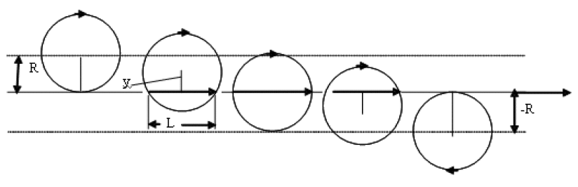
Figure 1: Cutting of Larmor orbits at the sample edge. Here, $R$ is the Larmor orbit radius, y is the distance from orbit centers to the sample edge, $L$ is the length of charge transfer for a given orbit along the edge.

Thus we have

$$M{\_}=1/2cNa^{2}\omega eR^{2}.$$

The compensating paramagnetic moment is the result of electron’s moving along edge cutting orbits. All orbits, that have a distance $y$ between their center and the cutting line ${\left|y\right|<R}$ (see Fig. 1), are cut and hence the number of cutting circles $n$ is

$$n=4a2RN=8NaR.$$

The average value $L_{av}$ of the shift $L(y)$ we find (see Fig. 2) as

$$L_{av}\mathbf{\mathit{\ }}=\frac{1}{2R}\int_{R}^{-R}L(y)dy\mathbf{\mathit{.}}$$

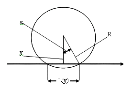
Figure 2: More detailed picture of a cutting orbit.

Replacing $y=R$cos$\alpha$, dy = $R$sin $\alpha d\alpha$ and $L(y)$ = 2$R$ sin $\alpha$, we obtain

$$L_{av}\mathbf{\mathit{\ }}=\mathbf{\mathit{\ }}\frac{1}{2R}\int_{0}^{\pi}{2R^{2}\sin^{2}\alpha d\alpha}=R\int_{0}^{\pi}{\sin^{2}\alpha d}\alpha\mathbf{\mathit{.}}$$

On the interval (0,$\pi)$

$$\int_{O}^{\pi}{\sin^{2}\alpha d\alpha\equiv\int_{0}^{\pi}{\cos^{2}\alpha d\alpha}},\text{ so that }L_{av}\mathbf{\mathit{\ }}=\mathbf{\mathit{\ }}\frac{\pi R}{2}.$$

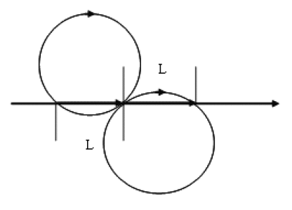
Figure 3: Two symmetrical orbits with the same $L$, situated “inside” and “outside” of a sample.

We find now the average velocity of electrons along the edge $v_{a}$ by combining the two cutting orbits of length $\alpha$ and  $2\pi-\alpha$ (see Fig. 3). They both have the same value of shift $L$ and whole time of moving on them is exactly the period $T=2\pi\mathbf{/}\omega\mathbf{\mathit{.}}$ So, the velocity $v\mathbf{=}2L/T$ and the average velocity is

$$v_{av}=2L_{av}/T=\omega R/2.$$

Thus, an average electron turns around the whole edge for the time $t^{\ast}=4a\mathbf{/}v_{av}\mathbf{=}8a/\omega R$ and the current of one electron is $e/t^{\ast}=e\omega R/8a$. Now we have to remember that the number of cutting circles is $n$ and every circle before cutting contains only one electron. Of course, the electron after cutting can find itself either inside or outside cutting line. Since the number of electrons is very high, the probability for electron to put itself inside the cutting line, i.e., in our square, is exactly one half. So, we have the number of skipping electrons exactly $n/2$, the whole paramagnetic current is

$$I_{+}=\frac{ne}{2t^{\ast}}=\frac{1}{2}Ne\omega R^{2},$$

$$M_{+}=1/2cNa^{2}e\omega R\mathbf{{}^{2},}$$

and

$$M_{+}=M{\_}.$$

Therefore, non-magnetic materials should remain completely non-magne-tic. It was, however, found long ago that a number of them, particularly bismuth, graphite, and some other, demonstrate a noticeable diamagnetism. It means that in those metals magnetic field can by some means increase the electron energy. But how can it be done?

L.D. Landau was the first who considered this problem from the quantum, or wave, mechanical point of view. From this point, a free moving particle can be associated with some fixed wavelength $\lambda$ (de Broglie wavelength) inversely proportional to the particle momentum. It is clear that for a free particle motion, $\lambda$, as well as the particle momentum and energy, can by, in general, arbitrary. However, if the motion is confined by a so-called potential box, then, roughly speaking, an integer number of wavelengths must be kept within a box. This means that $\lambda$ can no longer be an arbitrary, continuously varying parameter. Respectively, the particle energy can also change only by fixed portions, quanta. Of course, a piece of metal also represents a potential box for conduction electrons moving in it but its dimensions are, as a rule, so large that none of the electrons can cross it for its “free life”, or relaxation time $\tau$, which is the period between collisions with defects or impurities, inevitably present even in a very pure metal. For this reason, we can for sure neglect the size quantization. At the same time, the size of a Larmor orbit, inversely proportional to the magnetic field, is, as a rule, essentially less than dimensions of a real metallic sample, so that the probability of impurity or defect scattering at this orbit in a good sample is fairly low, especially in high magnetic fields. In other words, in this case the relaxation time $\tau$ is much more than the period of Larmor orbit 2$\pi$/$\omega$, i.e. $\omega\tau\gg 1$, and the electron motion at this orbit can be considered as a closed, finite one.

This approach brought L.D. Landau in 1930 [2] to the idea of equidistant, the so-called Landau levels. In the standard electron energy vs momentum dependence

$$E=\frac{1}{2m}p^{2}=\frac{1}{2m}(p_{x}^{2}+p_{y}^{2}+p_{z}^{2}),$$

the energy is a continuous function of any projection of the momentum $\eth$. In the magnetic field $H$, it can be presented in the form

$$E=\frac{1}{2m}(p_{\bot}^{2}+p_{\shortparallel}^{2}),$$

where $p_{\bot}$ and $p_{\shortparallel}$ are, respectively, normal and parallel projections of the momentum $\eth$ on the magnetic field direction. Instead of it, Landau obtained a principally new result:

$$E=\left(n+\frac{1}{2}\right)\hbar\omega+\frac{1}{2m}p_{\shortparallel}^{2}.$$

Here $n$ is an integer acquiring the values 0, 1, 2, …up to a some maximal one, $\hbar$ is the Planck’s constant divided by $2\pi,\omega=eH/mc$ is the cyclotron frequency, that is the frequency of electron rotation in a magnetic field, $m$ is the electron mass, and $c$ is the light velocity. In this case, the energy of electrons moving along closed orbits in the plane perpendicular to the magnetic field directions, can no longer change continuously. It changes by fixed portions, quanta, which magnitude $\hbar\omega$ is proportional to the magnetic field strength. It is essential that the minimal electron energy begins not from zero but $\hbar\omega/2$. At the same time, electron motion along the magnetic field remains unchanged.

Landau showed that the total energy of such quantized electron gas exceeds its classical value by a correction proportional to $H^{2}$, resulting in a negative magnetization, linear in magnetic field, and thus explaining the diamagnetism of free electrons. Besides this result, Landau found that for the magnetic field values large enough compared with the temperature, i.e. if

$$\hbar\omega\gg kT$$ (1)

($k$ is the Boltzmann constant), the field dependence of magnetic moments becomes essentially non-linear. The magnetic moment vs field dependence acquires a “fast periodicity”, or magnetization oscillations. In essence, it was a prediction of a new phenomenon. Unfortunately, at that time no ideas exist of a great variety of the Fermi surface shapes and sizes in metals, and the free electron model Landau based on, yielded extremely high requirements to the magnitude and uniformity of magnetic field, practically unachievable at that time, and he expressed a doubt concerning feasibility of experimental observation of this effect. Nevertheless, field oscillations of the magnetic moment with the period inversely proportional to the magnetic field, were soon discovered in bismuth by de Haas and van Alphen [3] and got the name of de Haas - van Alphen (dHvA) effect.

Later, the dHvA effect was observed in other metals as well but the oscillations were seen only in high quality single crystals and at very low temperatures. The oscillation amplitude dropped fast even at small temperature increase. The period of oscillations appeared to vary widely in different metals with the difference reaching several orders of magnitude. In some metals several periods were observed almost simultaneously (see Fig. 4), and the value of periods depended, as a rule, on the crystal orientation related to the magnetic field direction. It is not surprised that for a rather long time the magnetization oscillations were not directly associated with the Landau’s prediction.

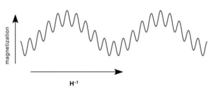
Figure 4: Example of dHvA oscillations with two frequencies in inverse magnetic field. The small period is about 10 times smaller than big one.

Such a versatility of experimental results managed to be understood only later, on the base of the LAKP (I.M. Lifshits, M.Ya. Azbel, M.I. Kaganov, V.G. Peschanskii) theory describing versatility of the Fermi surface shapes and sizes. In 1952 L. Onsager demonstrated first [4] that the constant period of magnetization oscillations as a function of inverse magnetic field, is inversely proportional to the area $A$ of extremal cross-section of the Fermi surface by a plane perpendicular to the magnetic field direction (see Fig. 5). The bigger is the area $A,$ the “faster” the magnetization oscillates. For instance, the dHvA from a Fermi surface like the dumbbell with two cross-sections is shown on Fig. 4. The inverse period – magnetic frequency – is given by the Onsager relation

$$F=\frac{c\hbar A}{2\pi e}.$$

Eventually, in 1955, I.M. Lifshits and A.M. Kosevich [5] developed the theory of metal magnetization (LK-theory). The authors advanced much further than Landau, obtaining a result adequate for any metal with arbitrary Fermi surface at arbitrary temperature, which, for the free electron model, naturally coincided with that of Landau. However, only due to the LK theory it became clear why the Landau diamagnetism might me anomalously large in several and why it is practically independent of temperature.

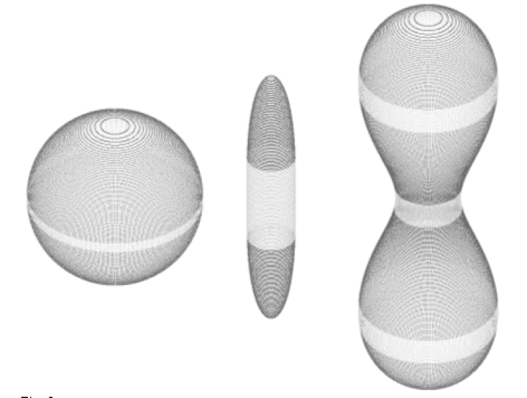
Figure 5: Different shapes of Fermi surfaces (schematically): spherical, long ellipsoid, dumbbell. The extremal belt is shown. The wider is a belt, the stronge is an oscillating contribution in energy and, consequently, dHvA amplitude.

Progress in theory served as a kind of impact for an unprecedented growth in the number of experimental investigations of metals in magnetic field at low temperature [6]. The measurements of magnetization oscillations have become one of the basic methods to study Fermi surface. During one decade, an enormous number of works was done and for all or almost all metals, at least those for which high quality single crystals could be grown, Fermi surfaces were “decoded”. And just here we are eventually approaching the main subject of this paper. It appears that importance of the dHvA effect is not restricted to its “benefits” in the Fermi surface decoding. The oscillating field dependence of the energy of metals in magnetic field is the base of some remarkable low-temperature phenomena being of independent interest. The formation of diamagnetic domains is definitely one of them.

So, let the formation of Landau levels in external uniform magnetic field $H$ cause in a metallic sample some oscillating addition $\tilde{\varepsilon}$ to the energy and, respectively, oscillating magnetization (the dHvA effect). This means that the magnetic field inside the sample, or magnetic induction $B$, differs slightly from the external field $H$. It is this difference

$$B-H=4\pi M$$

which does represent the oscillating magnetic moment. Thus, besides $\tilde{\varepsilon}$, we should also bear in mind the energy of excess magnetic field $B-H$ in the sample. Taking for simplicity our sample in the form of a long cylinder parallel to the magnetic field, we can write the total energy change per unit volume as the sum

$$\tilde{\varepsilon}+(B-H)^{2}/8\pi.$$ (2)

Since $\tilde{\varepsilon}$ is determined by the magnetic field $B$ acting on electrons, and oscillates in this field, it is evident that $B$ will change relative to $H$ always towards the nearest minimum of $\tilde{\varepsilon}$. The exact value of $B$ is obtained from the obligatory condition for this sum to acquire its minimal possible value, which requires vanishing its $B$-derivative. It means that

$$\frac{\partial\tilde{\varepsilon}}{\partial B}+\frac{B-H}{4\pi}=0,$$

or

$$B=H-4\pi\frac{\partial\tilde{\varepsilon}}{\partial B}\equiv H+4\pi M,$$

which gives us the expression for the magnetic moment $M(B)\equiv-{\partial\tilde{\varepsilon}}/\partial B$. The energy $\tilde{\varepsilon}$ is described by the exact LK formula, which takes into account both temperature and the Fermi surface shape but is very cumbersome. We take the simplest approximation for $\tilde{\varepsilon}$, sufficient for understanding the reasons of the phenomenon described, namely,

$$\tilde{\varepsilon}=a\mathrm{cos}\varphi\mathbf{,\ }$$

with the phase

$$\varphi=2\pi F/B\mathbf{.\ }$$ (3)

Here the amplitude $a$ is governed by various experimental conditions whereas the magnetic frequency $F$ is directly proportional to the area $A$ of extremal Fermi surface cross-section for the given metal (see Fig. 5), as mentioned above, represents Onsager relation

$$F=c\hbar A/2\pi e.$$

It is easy to see that if $a\ll 1$, the difference between $B$ and $H$ is negligibly small as compared to the oscillation period, that is the phase $\varphi$ remains practically unchanged at the replacement of $B$ by $H.$It seems evident that in this case the first derivative of $\tilde{\varepsilon}$ - the magnetic moment $M$ - and its second derivative – the differential susceptibility

$$\chi=\mathrm{dM/dH}\cong\chi_{B}=\partial M/\partial H\equiv{\partial}^{2}{\tilde{\varepsilon}}/\partial B^{2}$$

must have the sine or cosine shape as functions of the magnetic field. This means that the experimentally measured $M(H)$ and $\chi(H)$ dependences will have the same shape. This requirement is usually fulfilled but under some conditions it might be definitely not the case, which is very important for the domain formation.

From the expression for a phase (3) we have

$$\Delta\varphi=\frac{\partial\varphi}{\partial H}\Delta H=-\frac{2\pi F}{H^{2}}\Delta H$$

and for $\Delta\varphi$=2$\pi$

$$\Delta H=-\frac{H^{2}}{F}.$$

Here $H$ is the applied magnetic field, and negative sign shows the phase increase with inverse field. Note that this expression is insensitive to the difference $B-H$ that appears and disappears periodically and always vanishes at $\varphi$=2$\pi$n. So, one can already see that the “period” of oscillations in direct magnetic field $\Delta H$ decreases quadratically with the magnetic field. This means that oscillations become very “fast” at low field with a corresponding increase of the field derivatives and the differential susceptibility $\chi_{B}$ increasing, as a matter of fact, without limit. Of course, it is possible if and as long as the value of $\omega\tau$ remains exceeding one with the decrease of magnetic field, that is electrons still can perform more than one rotation in magnetic field. Let us look at consequences of such susceptibility growth. In the case considered, the field-induced change in magnetic induction will be essentially different depending on the sign of $\chi_{B}$. Indeed, this change

$$\delta B=\delta H+4\pi\delta M=\delta H+4\pi\frac{\partial M}{\partial B}\delta B\equiv\delta H+4\pi\chi_{B}\delta B,$$

i.e.

$$1+4\pi\chi=\frac{\partial B}{\partial H}=\frac{1}{1-4\pi\chi_{B}},$$

or

$$4\pi\chi=\frac{4\pi\chi_{B}}{1-4\pi\chi_{B}}.$$

From this it follows that if the absolute value of $\chi_{B}$ grows, the denominator increases, $\partial B/\partial H\rightarrow 0$ and 4$\pi\chi\rightarrow-1$ for negative $\chi_{B}$, while for positive $\chi_{B}$ the denominator vanishes and at $\chi_{B}\rightarrow$ 1/4$\pi$ $\partial B/\partial H\rightarrow\infty$, so that the sample induction has to increase like a jump. As a result, instead of a sine-like (harmonic) signal, the following picture should be observed in dHvA experiments. In the vicinity of a minimum of $\tilde{\varepsilon}$, where $\chi_{B}$ $<0$, $B$ remains practically unchanged over almost all period, and 4$\pi\delta M\approx-\delta M$, and 4$\pi\chi\cong$ $-1$ (almost as in a “superconductor”). But in the vicinity of a maximum of $\tilde{\varepsilon}$, where $\chi_{B}$ is positive, the induction $B$ and, hence 4$\pi M$,

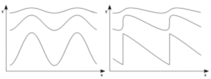
Figure 6: Transformation of the shape of dHvA signal $y(x)$ when passing from $M(B)$ to $M(H)$. In the left panel, the x-axis represents the magnetic field inside of a sample, i.e. the induction $B$. In the right panel, the $x$-axis represents the applied magnetic field $H$, reproducing a real magnetization measurement. In both pictures, the curves $y(x)$ are shown (from up to down) for increasing of $a$: $a\ll 1,$ $a=1$ and $a\gg 1$, ($a$ can increase, for instance, with temperature decrease). With this transformation, every point of the left curves is shifted by the value of its respective $y$-coordinate either to the left ($y>0$) or to the right ($y<0$), according to $H=B-4\pi M(B$). The most upper curve almost does not change with this transition. Note the jumps $\Delta y=\Delta B$ on the lower right curve.

increase stepwise by $\Delta B$ approximately equal to the oscillation period (see Fig. 6), as soon as

$$\chi_{B}\geq 1/4\pi.$$ (4)

Such a saw-toothed $M(H)$ dependence with almost vertical induction steps was first observed by D. Shoenberg in the noble metal samples [6]. As we see, metals in magnetic field demonstrate quite a “reasonable” behavior: the sample induction $B$ changes in such a manner that the energy stays maximally long near its minimal value while the high energy intervals $\Delta B$ (strictly speaking, these are the regions of absolute instability) are jumped over (see Fig. 7).

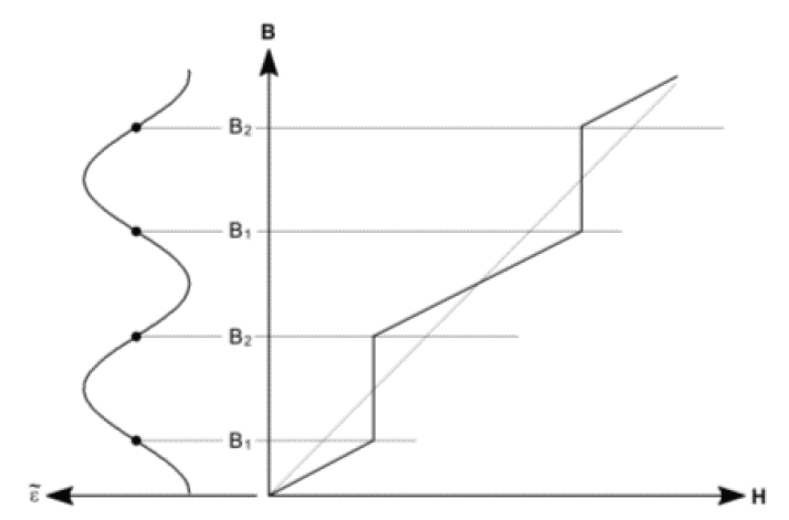
Figure 7: On the right: $B(H)$ dependence in a long sample for $y(x)$ given by the lower right curve of Fig. 6. The diagonal $B=H$ crosses the curve at $M=0$. The function $\tilde{\varepsilon}(B)$ is shown at the left. The regions of high energy (absolute instability) are absent in the sample as they “jump” by $\Delta B$.

By now, one can already “guess” (all of us are slow on the uptake) that the choice of some other geometry of experiment, say, by using a planar sample normal to the field, rather than a cylinder parallel to it, might provoke a different scenario of events. Indeed, in the planar geometry with all sample dimensions considerably exceeding its thickness, the compulsory continuity of the normal component of $B$ results in the requirement

$$B=H$$ (5)

Since $H$ varies continuously, therefore in this geometry of experiment any jump in $\Delta B$ cannot exist in principle. It means, in turn, that the above-mentioned “reasonable” behavior of metal cannot presumably be realized: the induction must acquire all consecutive values near the energy maximum, which is definitely unfavorable. This is what to think about. Looking ahead, we declare at once that, thanks to domains, a metal manages to behave “reasonably” and rush an unfavorable region $\Delta B$ by in this case as well. Nevertheless, several years had passed until Condon formulated the idea of domain formation [1].

It is to be said that this idea was preceded and, to some extent, stimulated by numerous experiments with beryllium single crystals. The Fermi surface of this metal contains the so-called “cigars” with the shape quite similar to a long cylinder. That is why in this metal amplitudes of the dHvA and other effects in magnetic field are very high. Besides dHvA, where the above-mentioned stepwise behavior of magnetic moment is well-pronounced, many other effects, including the transversal magnetoresistance, were measured. Very large amplitude of these oscillations is a specific feature of the beryllium Fermi surface. It is essential that what is measured, is a long strip or a rod perpendicular to the external magnetic field. That is, absolutely unusual magnetic field dependence of the amplitude of these oscillations could be explained only by the domain formation in a sample, or, in other words, breaking it up into areas of different magnetization.

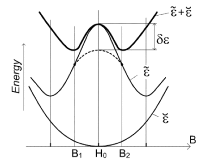
Figure 8: The energy variation as a function of $B$ is shown for a small region slightly larger than one period of oscillating function $\tilde{\varepsilon}$. The external magnetic field $H_{0}$ is chosen to be exactly at the maximum of $\tilde{\varepsilon}$. The parabola $\mathord{\buildrel\lower 3.0pt\hbox{$\scriptscriptstyle\smile$}\over{\varepsilon}}$ represents the variation of the magnetization energy for a very long sample in applied magnetic field $H_{0}$. The upper curve shows the sum $\tilde{\varepsilon}+\mathord{\buildrel\lower 3.0pt\hbox{$\scriptscriptstyle\smile$}\over{\varepsilon}}$. It has minima at $B_{1}$ and $B_{2}$. The energy of a plate-like sample with domains is shown by the dashed line.

To understand it better, let us appeal to a graphical presentation of the full energy change (2) depending on the magnetic field in the sample, that is on $B$. The graph (Fig. 8) shows a small region of the variations of $B$ in the vicinity of a given external magnetic field $H_{0}$, that is exactly corresponds to an immediate maximum of the oscillating function $\tilde{\varepsilon}$. The parabola $\mathord{\buildrel\lower 3.0pt\hbox{$\scriptscriptstyle\smile$}\over{\varepsilon}}=(B-H_{0})^{2}/8\pi$ depicts the second term in (2), that is the magnetization current energy caused by the difference ($B-H_{0}$ ) in a sample. We emphasize that for the time being we are dealing again with a long sample oriented along the magnetic field. The upper curve shows $\tilde{\varepsilon}+\mathord{\buildrel\lower 3.0pt\hbox{$\scriptscriptstyle\smile$}\over{\varepsilon}}$ - the total energy (2). Our figure corresponds to the situation when the curvature of parabola is obviously less than the curvature of $\tilde{\varepsilon}$ in a maximum, so that the condition (4) is satisfied. Only in this case the sum $\tilde{\varepsilon}+\mathord{\buildrel\lower 3.0pt\hbox{$\scriptscriptstyle\smile$}\over{\varepsilon}}$ has two symmetric minima in the points $B_{1}$ and $B_{2}$. (In the opposite case, when 4$\pi\chi<1$, the curve $\tilde{\varepsilon}+\mathord{\buildrel\lower 3.0pt\hbox{$\scriptscriptstyle\smile$}\over{\varepsilon}}$ has always only one minimum). Let us remind that we have chosen $H_{0}$ exactly in the maximum and hence the energies in these minima coincide. Of course, if one shifts an applied magnetic field $H$ slightly left of $H_{0}$, with a simultaneous shift of the parabola $\mathord{\buildrel\lower 3.0pt\hbox{$\scriptscriptstyle\smile$}\over{\varepsilon}}$, then $\tilde{\varepsilon}+\mathord{\buildrel\lower 3.0pt\hbox{$\scriptscriptstyle\smile$}\over{\varepsilon}}$ will become slightly warped, with energy in the minimum $B_{1}$ becoming less than in $B_{2}$. A similar right shift will cause an opposite kind of warping and lowering the minimum $B_{2}$ below $B_{1}$. Since the state of a metal always corresponds to minimal energy, as soon as the external field crosses the point $H=H_{0}$, the sample magnetic induction jumps from $B_{1}$ to $B_{2}$. The negative magnetization $B_{1}-H_{0}=$4$\pi M_{1}$ at this point will, respectively, change into the positive one $B_{2}-H_{0}=$ 4$\pi M_{2}$, in other words, the sample jumps from a dia- to a paramagnetic state.

Now we look at the domain formation in this picture (Fig. 8). To do it, we take the same crystal with the same crystallographic orientation related to the magnetic field, that is leave $\tilde{\varepsilon}$ unchanged, but reshape the sample transforming it into a large thin plate perpendicular to the field, so that, with the well known boundary condition, equality (5) must be fulfilled everywhere. This means $B-H=0$, allowing us to remove mentally the parabola $\mathord{\buildrel\lower 3.0pt\hbox{$\scriptscriptstyle\smile$}\over{\varepsilon}}$. As a result, the sum $\tilde{\varepsilon}+\mathord{\buildrel\lower 3.0pt\hbox{$\scriptscriptstyle\smile$}\over{\varepsilon}}$ (2) simply coincides now with $\tilde{\varepsilon}$. By comparing this result with the previous one, that is with the curve $\tilde{\varepsilon}+\mathord{\buildrel\lower 3.0pt\hbox{$\scriptscriptstyle\smile$}\over{\varepsilon}}$ on the figure, we see that over a large range of magnetic fields in the vicinity of $H_{0}$, the energy of metal becomes considerably higher than the minimal value realized in a thin sample. This exceeding is maximal at $H=H_{0}$ being equal to $\delta\varepsilon$. The question is if it is possible to reduce the energy by dividing our plate into a set of thin regions – “domains”. Let their length, which is the plate thickness, be much larger than the “domain” thickness, in which case the cross-section of such a “domain” looks similar to that for a solitary long sample oriented along the field. That is why we can apply the formula (2) that is the curve $\tilde{\varepsilon}+\mathord{\buildrel\lower 3.0pt\hbox{$\scriptscriptstyle\smile$}\over{\varepsilon}}$ for each of them. If we now break them up into two sorts with the induction values $B_{1}$ and $B_{2}$ and mix carefully to make these sorts alternating everywhere, then these domains (already without quotation marks) will represent what is called Condon’s domains. Since domain size and number are for both sorts equal, in each sample region much larger than the domain size the average induction remains equal to $H_{0}$, that is the condition (5) is now satisfied on average throughout the whole sample. In each domain the energy (2) corresponds to a minimum, which means that for the whole plate the energy gain will be the same, namely $\delta\varepsilon$. Fig. 9 schematically shows such domain structure. If the magnetic field changes towards $B_{1}$ or $B_{2}$, then the domain sizes vary correspondingly, increasing the thickness of one sort of domains and decreasing the other in such a way that the condition (5) remain on average satisfied. Simple calculations show that formation of domains with the constant values $B_{1}$ and $B_{2}$ in each sort of them becomes more profitable than the uniform state for all values of magnetic field in region $B_{1}<H<B_{2}$. This energy gain is shown in the Fig. 8 by the dashed line.

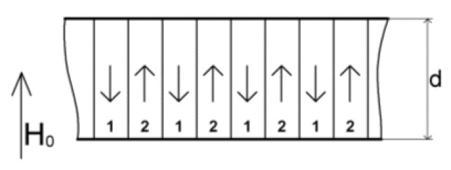
Figure 9: Schematic picture of the domain structure in a plate-like sample. In reality, the period of the structure is much smaller than the thickness $d$. The arrows show directions of magnetization in phases 1 and 2.

In 1966 Condon formulated first the idea of such domains, and already in two years Condon and Walstedt [7] demonstrated the domain formation in nuclear magnetic resonance (NMR) experiments in silver. Let us remind that nuclear magnetic moment, or spin, rotates in the magnetic field with the angular frequency of such rotation, or precession, strictly proportional to the field strength. If, besides, an additional high-frequency electromagnetic field effects a nucleus, a resonant absorption of electromagnetic energy by this nucleus occurs as soon as the field frequency coincides with the precession frequency. The frequency of a.c. field, created usually by a small coil winded sometimes directly on a sample, can be measured with enormous precision, and hence NMR gives the opportunity to measure magnetic field in a medium with the same precision (of course, only if one succeeds in measuring the absorption itself, which is not a simple task). In a uniform field, a narrow NMR line is observed, whereas any non-uniformity broadens this NMR peak (line). Condon and Walstedt were the first who observed two coexisting resonant frequencies, that is the line splitting. At changing the external magnetic field the effect arose periodically with the period corresponding to the dHvA period in the same sample, while the magnitude of splitting had the order of half a period and corresponded to two sorts of domains with induction values $B_{1}$ and $B_{2}.$

Unqualified success of this experiment was a well-deserved result of overcoming a large number of difficulties. Besides all already mentioned conditions of domain formation including low temperature of 1.4 K, very high magnetic field uniformity with spatial fluctuations essentially less than the splitting value $\delta B=B_{2}-B_{1}=12$ Gauss against the field of 9 T, and very high perfection of a Ag single crystal, an additional difficulty consisted in detecting of NMR in a metal, especially in a very pure metal, as in the experiment. The case is that a.c. electromagnetic field penetrates a metal only at very small depth, the so-called skin layer. That is why only small number of nuclei near the sample surface contribute to absorption. With the account of all above-mentioned factors, the authors presumably had very few chances for success, thus the result speaks for itself.

The authors naturally tried to obtain the same result for beryllium, the “champion” among metals with the highest amplitude of the dHvA effect, but suffered a reverse. The method did not work. Contrary to silver where the nuclear magnetic moment is equal to $1/2$ and its projection to the magnetic field has only two allowed values: along and opposite to the field, this moment for beryllium is equal to $3/2$, so that initially, without any domains, the so-called quadrupole splitting of the NMR line already exists. This is one more difficulty in observation of domains in many metals by the NMR method. All the problems discussed where presumably the reason why after a success with silver and failure with beryllium no single work devoted to revealing diamagnetic domains by the NMR method appeared in the literature. The progress and all recent achievements in visualization of diamagnetic domains is related to a new investigation method – Muon Spin Rotation, called $\mu$SR [8]

This method was developed at the “interface” between two branches of physics – nuclear physics and condensed matter physics, and actually is almost complete analog of the NMR. As early as in 1979, Yu. Belousov and V. Smilga suggested to use it for observation of Condon domains [9]. The technique of that time, however, was not yet adequate, “interface” was not formed, and their work remained, alas, unnoticeable. 16 years later the idea of using the $\mu$SR method for domain observation was reborn, this time with a project proposed by G. Solt at the Paul Scherrer Institute, Switzerland, where this method is of a wide use. Experiments in beryllium were a success [10], and splitting of the $\mu$SR peak, similar to that for NMR, caused by diamagnetic domain formation, was observed.

The $\mu$SR method, in spite of its direct analogy with NMR, has, of course, a number of distinctions as well. Muons are unstable elementary particles with the lifetime close to two microseconds. They represent an outcome of activity of a powerful accelerator. A positive muon, having sufficiently high initial energy, can penetrate the sample at fairly large depth and stop at some interstitial remaining there during the whole lifetime. It also has a spin precessing in exact correspondence with the local value of magnetic field. Decay of a muon creates a positron, or anti-electron, which rushes our mostly in the direction of its spin and is registered by one or another detector. In the experiment, a great number of muons is detected, with all their spins rotating from strictly the same starting position. If all muons are in the same magnetic field, then the number of registered events in each detector will oscillate with time with the precession frequency $f$ exactly determining the magnitude of this magnetic field, that is $f=gB$, where the constant $g$ is well known for muon. In this methods there is no need in a.c. electromagnetic field since the precession frequency is measured directly, and therefore the first difficulty of NMR measurements caused by a skin-layer no longer exists. The second difficulty is absent as well since in any matrix the “job” was made by the same “test” instrument with the spin $1/2$. The fact that spin precession occurs far enough from the sample surface, represents the third important advantage of this method, at least for this problem. As a result, by analogy with NMR, the width of $\mu$SR peak corresponds to the amplitude of magnetic field non-uniformity. If now the sample becomes stratified into two phases with the magnetic field values $B_{1}$ and $B_{2}$, that is domains, then one part of muons will find themselves in the field $B_{1}$ and the other part – in the field $B_{2}$, which will result in two precession frequencies and, respectively, in a splitting of the $\mu$SR peak into two peaks.

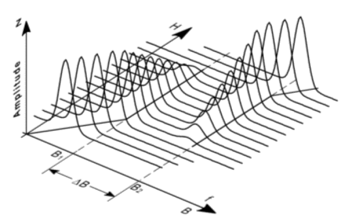
Figure 10: Several ${\mu}$SR spectra over a small region of applied magnetic field $H$ near the onset of Condon domains. (The spectra are shown without noise). The peaks of the spectra without domains are always along the diagonal $B=H$. In the domain region, there are two peaks of $f_{1}$ and $f_{2}$ corresponding to $B_{1}$ and $B_{2}$.

The Fig. 10 demonstrates the results of $\mu$SR experiment on a crystalline plate of beryllium [11]. Each time when $H$ goes through the region $B_{1}<H<B_{2}$, the spectrum will split into two peaks with the fixed frequencies corresponding to $B_{1}$ and $B_{2}$. While the field changes, the amplitude of one peak decreases and the amplitude of the other increases, which corresponds to the change of relative volumes occupied by these two phases. Analysis of the data available confirms that the relationship (5) is always exactly fulfilled. At any other values of magnetic field beyond the given range, a standard narrow peak is observed with the frequency corresponding to this field.

Now we can say that a successful result of the experiments with beryllium is quite natural since this material, as it has been already mentioned, is a “champion” in the dHvA amplitude. In the magnetic field 3T, diamagnetic domains exist up to the temperature $\sim$ 3K. For the most other metals, however, the dHvA amplitude is considerably less than for beryllium. As a rule, it remains under all conditions noticeably less than one tenth of period. But it is well known, that the condition (4) or $a\geq$1 (which is the same for a sine-shape dHvA signal) is satisfied if the amplitude $4\pi M\geq P/2\pi$ ($P$ is the period). At first glance, Condon domains seem impossible under these conditions representing a very rare phenomenon, which is, however, not the case. Actually, the shape of dHvA signal at very low temperatures is already essentially different from a sine curve. A careful analysis shows that even for a very small dHvA amplitude, the condition (4) at sufficiently low temperatures will be satisfied without fail, though the range $B_{2}-B_{1}$ in this case may be very narrow, essentially less than the period. Therefore, the difference in magnetization and the $\mu$SR peak splitting are extremely small, and experimental observation of domain formation becomes much more difficult. It requires both absolutely perfect crystals and more sophisticated measuring technique.

Just such experiments have been recently performed in the same the Paul Scherrer Institute. The mentioned more sophisticated technique making it possible to diminish essentially the noise level, the so-called MORE, was worked up at this institute. Formation of diamagnetic domains was discovered in all measured single crystals of tin, aluminum, indium and lead. (They were grown in the P.L. Kapitsa Institute of Physical Problems almost 30 years ago). The condition for domains to exist was restricted to several tenth of Kelvin temperature. Success of this work [11] was naturally based on the many year work of numbers and numbers of physicists. Now one can be sure that diamagnetic, or Condon, domains represent a phenomenon spread as widely as the dHvA effect though requiring much more rigid conditions for their observation.

Two more questions should be mentioned, at least casually, in this paper. The first, quite natural question is that of a mechanism of electric current in a rather thin, of order of one micron, domain wall. So, in beryllium at $B_{2}-B_{1}$ around 30 G, the current density in the wall has to be $\cong 3.10^{5}$À/cm². It is a very large value. In ordinary magnetic domain formed by spins (atomic magnetic moments) with opposite direction, this mechanism is clear: currents circulating in adjacent domains, respectively, clockwise and anticlockwise, add at the boundary forming thus a magnetization current. But in our case Larmor rotation of electrons is identical both sides of the boundary so that in this sense the boundary is not marked out. The answer consists in the fact that in the dHvA effect not only magnetization but also the crystal size is varied, which is knows as the striction effect. The case is that the phase of oscillating energy $\varphi$ =2$\pi F/B$ (3) is determined not only by the induction $B$ but also by the value of $F$, that is by the Fermi surface cross-section, which, in turn, depends on the sizes of a crystal cell. That is why a metal in the external magnetic field changes not only its magnetization but also the cross-section, or the volume, of the Fermi surface by a proper dimension changes, in order to approach the energy minimum “faster”. While jumping from $B_{1}$ to $B_{2}$, this striction also suffers a jump. In this process, opposite magnetization corresponds, in some sense, to opposite deformation. In domains, on the contrary, variation of deformation from one value to the other must occur in a domain wall more or less smoothly. Now it is clear that larger Fermi surface volume, that is larger charge density, corresponds to a diamagnetic phase while smaller volume corresponds to a paramagnetic phase with the charge density gradient in the domain wall providing the required magnetization current. Of course, striction is directly proportional to magnetization and has a very small magnitude. So, in the above-mentioned beryllium with a record magnitude of effects the deformation has the order of one per million. Thus, formation of the domain structure is also accompanied by a corresponding, unfortunately very small, periodic deformation of the unite cell size and, moreover, relief at the sample surface. This makes it very difficult for observation even by a heavily aided eye.

This is not the only place where deformation, or formation of domains from different density phases, reveals itself. Measurements of magnetostriction in a beryllium plate resulted in discovery of an absolutely amazing property of the formed domain structures, which cannot be named other than “supersoftness” [12]. It should be noted that beryllium by itself is a very hard metal, inferior by this property only to tungsten and iridium. Its Young’s modulus is almost one order of magnitude higher than that of copper. Nevertheless, a copper needle of a regulating screw pressing the beryllium plate to the measuring instrument with minimal force, periodically, at the formation of domain structure, comes down the sample at a rather noticeable depth. The depth of a “pit” under the needle, which, of course, heals instantly as soon as the sample becomes single-phased, corresponds to at least hundredfold drop in the Young’s modulus. This unique behavior can be explained only in terms of corresponding domain restructuring in the vicinity of the needle.

The second question is as follows. In our opinion, there is a direct analogy between described diamagnetic domains and alternation of normal and superconducting phases in the known intermediate state of a type I superconductor. Indeed, a long thin cylindrical superconducting sample oriented along the magnetic field, at some critical field $H_{c}$ demonstrates a stepwise transition from the superconducting state with $B_{1}=0$ into the normal one with $B_{2}=H_{c}$. Of course, both states correspond to a minimum of energy. If we now take a sample of the same metal but in the shape of a thin plate perpendicular to the field, pure geometric considerations will again bring us to the necessary condition (5). However, in the magnetic field interval between $B_{1}$ and $B_{2}$, that is between zero and $H_{c}$, a uniform solution will possess some excess energy. Minimal energy will be achieved by fragmentation of a sample into alternating “domains” with the induction $B_{1}$=0 and $B_{2}=H_{c}$, that is into normal and superconducting phases, exactly as in the case of diamagnetic domains. In this case the condition (5) is again fulfilled on average on the account of proportional changes of the relative volumes of the phases. Actually the analogy is even closer. From the analysis of domain structure periods it results that these may be very close in samples of the same thickness. This means that domain structures of either shape may be rather similar to such different phenomena as superconductivity and dHvA effect. Unfortunately, this is the end of analogy and remaining distinctions have a fundamental character. If the “magnetic contrast”, that is the ratio of $B_{2}-B_{1}$ to $B_{2}$, is almost hundred percent for the intermediate state image, then for Condon domains it is so far 0.1% at best. Besides, the magnetic field itself is here hundred times more, which creates an additional obstacle for the magnetooptical method used for imaging. However, the principal possibility of obtaining a diamagnetic domain image remains, which gives ground for some optimism.

In conclusion, a couple of words should be said regarding “practical application” of Condon domains. They give an absolutely unexpected possibility of direct approach to the question of compressibility of metals. It appears that if compressibility of metals $\beta_{\mathrm{met}}$ is governed exclusively by the kinetic energy of the electron gas, i.e. $\beta_{\mathrm{met}}=\beta_{\mathrm{el},}$ then only in this case no contact voltage exists between domains and, hence, the domain wall interior contains no electric field.

In 1957 M.I. Kaganov, I.M. Lifshits, and K.D. Sinel’nikov predicted theoretically [13] the effect of Fermi level oscillations with magnetic field

$$\delta\mu_{KLS}(H)=\frac{\partial\tilde{\varepsilon}(H)}{\partial N},$$

where the energy $\tilde{\varepsilon}$ already mentioned above, is described by the exact LK formula and $N$ – is the density of electrons. The result was obtained for the case of constant $N$. Nevertheless, as a result of striction, the volume $V$ changes, $N=N_{0}/V,N_{0}$ is a constant quantity of electrons in a crystal, and the complete change of Fermi level is

$$d\mu=\delta\mu_{KLS}+\frac{\partial\mu}{\partial V}\delta V,$$

where $\delta V$ is the striction in the crystal. We can write

$$\delta\mu_{KLS}=\frac{\partial\tilde{\varepsilon}}{\partial V}\frac{\partial V}{\partial N}=\frac{V}{N}\delta\tilde{p},$$

where

$$\delta\tilde{p}=-\frac{\partial\tilde{\varepsilon}}{\partial V},$$

and

$$\delta V=\frac{\partial V}{\partial p}\delta p\ast,$$

where $\delta p$* is the pressure decrease caused by striction. The total variation of pressure for a sample with free boundaries is zero

$$\delta\tilde{p}+\delta p\ast=0,$$

and

$$d\mu=\frac{V}{N}\delta\tilde{p}(1+N\frac{\partial\mu}{\partial V}\beta_{\mathrm{met}}).$$

Here the $\beta_{\mathrm{met}}$ is a compressibility of the metal which can be found in a Handbook. Now we rewrite

$$\frac{\partial\mu}{\partial V}=-\frac{\partial p}{\partial N},$$

and from

$$\frac{\partial N}{\partial p}=\frac{\partial(N_{0}/V)}{\partial p}=-\frac{N_{0}}{V^{2}}\frac{\partial V}{\partial p}=-\frac{N}{V}\frac{\partial V}{\partial p}=N\beta_{\mathrm{el}}$$

we have

$$\frac{\partial\mu}{\partial V}=-\frac{1}{N\beta_{\mathrm{el}}}.$$

Here $\beta_{\mathrm{el}}$ is a compressibility of electron gas which could be found, in principle, from an equation of state for electron gas in this metal. Of course, $\beta_{\mathrm{el}}$ is connected with a kinetic energy of electrons only. At least, we have for the net shift of Fermi level

$$d\mu=\beta\mu_{KLS}(1-\frac{\beta_{\mathrm{met}}}{\beta_{\mathrm{el}}}).$$

Therefore, one can, in principle, find the value of $\beta_{\mathrm{el}}$ from a contact voltage measurement. In the case $\beta_{\mathrm{met}}=\beta_{\mathrm{el}}$ the first derivative of exchange energy has a maximum and only kinetic energy of electrons contributes in compressibility. Only in such case the effect of Fermi level oscillations is wholly compensated as a result of magnetostriction gaining no contact voltage between domains, no electrical field in domain walls, and no extra energy. Maybe just for this not trivial reason we can see the Condon domains in all metals [11].

On the other hand, if we assume that the whole magnetization current in a domain wall is a result of only charge density gradient, that is domains are actually only diamagnetic, with negligible role of spins, it appears that compressibility of metals is completely determined by the construction of their Fermi surface.

Indeed, let the difference in magnetization between neighboring domains be really caused by deformation accompanied by electron density changes. Then the magnetization current density in a domain wall can be described by the formula [14]

$j_{m}=c$ curl $\sum\limits_{k}{n_{k}(r)\mu_{k}}$

Here, $n_{k}(r)$ is the number of Larmor orbits corresponding to the $\mu$ magnetic moment of a unit volume $\mu_{k}$, $c$ is the light velocity. Let us integrate j_m over the domain wall thickness from one domain to another taking into account that the orbital magnetic moments of all electrons are parallel to the magnetic field. This gives the magnetization current in the wall related per unit length of this wall along the field,

$J$= $c\sum\limits_{k}{(N_{2}-N_{1})_{k}\mu_{k}}$

where $(N_{1},_{2})_{k}$ are the volume densities of charges with magnetic moment $\mu_{k}$ in neighboring domains. Since the $\delta N$ difference is small, all orbits can be considered to be situated on the Fermi surface. The characteristic values can be estimated as follows. The magnetic moment of a Larmor orbit is

$$\mu_{k}=\frac{J_{L}S_{L}}{c},$$

where $J_{L}=\omega_{c}e/2\pi$ is the current on Larmor orbit and $S_{L}=\pi R_{H}^{2}$ is its area. Here $\omega_{c}=eH/mc$ is the cyclotron frequency, $e$ is the charge of the electron, $R_{H}=v_{\bot}$/$\omega$ is the Larmor radius, and $v_{\bot}$ is the velocity of electrons on the Fermi surface in the direction normal to the field. We can write the complete current $J$ in the domain wall per unit wall length in the magnetic field direction as

$$J=\delta N\frac{c}{H}\frac{mv_{F}^{2}}{2}C_{FS}=\delta N\frac{c}{H}\varepsilon_{F}C_{FS},$$

where $\delta N$ is the total difference of the numbers of charge carriers (electrons and holes) in neighboring domains, that is, the difference of the Fermi surface volumes in these domains, and the constant $C_{FS}$ is a result of averaging $v_{\bot}$ over the Fermi surface. As the induction jump between neighboring domains is

$$\Delta B=4\pi\Delta M=(4\pi/c)J,$$

where $J$ is just the current in the domain wall, we have

$$\Delta MH=\delta N\varepsilon_{F}C_{FS}.$$

The changing of charge density $\delta N$/$N_{0}$ can always be considered equal to $\gamma C_{\gamma}$ where $\gamma$ is striction and $C_{\gamma}$ is the coefficient unambiguously determined by the Fermi surface shape. (Clearly, this coefficient is equal to 3 in the model of free electrons). So, we can rewrite

$$\Delta MH=\gamma N_{0}\varepsilon_{F}C_{FS}C_{\gamma}.$$

At least, we have the well-known formula for striction [6]

$$\gamma=\frac{MH}{Y}\frac{\partial\ln A}{\partial\gamma}=\frac{MH}{Y}C_{A}.$$

Here $Y$ is Young’s modulus and the constant $C_{A}$ shows a changing of Fermi surface cross-section $A$ with striction $\gamma$. As a result, we have

$$Y=N_{0}\varepsilon_{F}C_{FS}C_{\gamma}C_{A},$$

where all coefficients are fully determined by the Fermi surface structure. Here, $\varepsilon_{F}$ is the kinetic energy of electrons on the Fermi surface, that is, $\varepsilon_{F}=\hbar^{2}k_{F}^{2}/2m$. For instance, for beryllium [12], the correct Young’s modulus value was obtained in such a simple way.

To summarize, we can say that no wonderful Condon domains are connected with a compressibility of metal for its appearance is directly connected with deformation. But the concept described above in a very simple way, shows that conduction electrons should fully determine its compressibility coefficient. Of course, it is much more strong result and the result is strange. At the same time, the formation of diamagnetic domains is doubtless characteristic for all metals; the only problem is the extremal difficulty of creating the necessary conditions for most of them. As mentioned, such domains were observed in silver, beryllium, tin, lead, indium and aluminum. In other words, the very possibility of the existence of diamagnetic domains lends support to the point of view according to which conduction electrons should fully, or almost fully determine the compressibility of metals. Of course, it is very difficult to say now to what extent this conclusion is quantitatively accurate.

I am indebted to L. Maksimov, D. Sholt, V. Mineev, A. Dyugaev for interesting discussions of the questions touched upon and to M. Schlenker for useful remarks.

References

- [1] J.H. Condon, Phys. Rev. 145, 526 (1966).
- [2] L. Landau, Z. Phys. 64, 629 (1930).
- [3] W.J. de Haas and P.M. van Alphen, Proc. Neth. Roy. Acad. Sci. 33, 1106 (1930).
- [4] L. Onsager, Philos. Mag. 43, 1006 (1952).
- [5] I.M. Lifshits and A.M.Kosevich, Sov. Phys. JETP 2, 636 (1956).
- [6] D. Shoenberg, Magnetic Oscillations in Metals (Cambridge Univ. Press, Cambridge, 1984).
- [7] J.H. Condon and R.E.Walstedt, Phys. Rev. Lett. 21, 612 (1968).
- [8] A. Schenck, Muon Spin Rotation Spectroscopy (Hilger, Bristol, 1986).
- [9] Yu.M. Belousov and V.P. Smilga, Sov. Phys. Solid State 21, 1416 (1979).
- [10] G. Solt, C. Baines, V. Egorov, D. Herlach, E. Krasnoperov, and U. Zimmermann, Phys. Rev. Lett. 76, 2575 (1996).
- [11] G. Solt and V.S. Egorov, Physica B 318, 231 (2002).
- [12] V.S. Egorov and Ph.V. Lykov, Sov. Phys. JETP 94, 162 (2002).
- [13] M.I. Kaganov, I.M. Lifshits, and K.D. Sinel’nikov, Sov. Phys. JETP 5, 500 (1957).
- [14] D.A. Frank-Kamenetskii, Lectures on Plasma Physics (Atomizdat, Moscow, 1968).