Photon Channelling in Foams

Abstract

Experiments by Gittings, Bandyopadhyay, and Durian [Europhys. Lett. 65, 414 (2004)] demonstrate that light possesses a higher probability to propagate in the liquid phase of a foam due to total reflection. The authors term this observation photon channelling which we investigate in this article theoretically. We first derive a central relation in the work of Gitting et al. without any free parameters. It links the photon’s path-length fraction $f$ in the liquid phase to the liquid fraction $\varepsilon$. We then construct two-dimensional Voronoi foams, replace the cell edges by channels to represent the liquid films and simulate photon paths according to the laws of ray optics using transmission and reflection coefficients from Fresnel’s formulas. In an exact honeycomb foam, the photons show superdiffusive behavior. It becomes diffusive as soon as disorder is introduced into the foams. The dependence of the diffusion constant on channel width and refractive index is explained by a one-dimensional random-walk model. It contains a photon channelling state that is crucial for the understanding of the numerical results. At the end, we shortly comment on the observation that photon channelling only occurs in a finite range of $\varepsilon$.

I Introduction

Aqueous foams consist of gas bubbles separated by liquid films Weaire1999 . In dry foams, these bubbles are deformed to polyhedra. Always three films meet in the so-called Plateau borders which form a network of liquid channels throughout the foams. Their opaque appearance identifies them as multiply scattering media. Moreover, careful light-scattering experiments show that light transport has reached its diffusive limit in foams Durianold ; Ern ; Hoehler ; Gopal99 ; durApp which means that photons perform a random walk. Diffusion of light is well established in colloidal systems DWS , where light is scattered from particles, or in nematic liquid crystals DWSnematic , where scattering occurs from fluctuations in the local optical axis. Diffusing-wave DWS and diffuse-transmission spectroscopy Kaplan94 provide non-invasive probes of structure and dynamics in bulk samples. While these methods have already successfully been applied to monitor the internal dynamics of foams Durianold ; Ern ; Hoehler ; Gopal99 , no clear understanding has emerged so far about the basic mechanism underlying the random walk of photons in these cellular structures. Estimates for the scattering from Plateau borders do not seem to be in accordance with experiments durApp ; Gittings2004 . Scattering from vertices formed by four meeting Plateau borders would be another possibility Skipetrov02 . On the other hand, since gas bubbles in foams are much larger than the wavelength of light, one can use the laws of ray optics to follow the photons on their random walk as they are reflected by the liquid films Miri03 ; Miri04 ; Miri05 ; Miri05a .

The work presented in this paper was initiated by a very inspiring publication of Gittings, Bandyopadhyay, and Durian published under the same title Gittings2004 . The authors argued that total reflection of light at the liquid-gas interface in a foam should increase the probability of photons to propagate in the liquid phase, made up by thin films and Plateau borders, and they termed this effect photon channelling. By measuring the absorption of light in foams with strongly absorbing liquid, they determined the fraction $f$ of a photon’s path that lies in the liquid. Equal distribution of the photons throughout the foam would give $f=\varepsilon$, where $\varepsilon$ is the liquid fraction in the foam. However, the authors found that in a certain range of $\varepsilon$ the path-length fraction $f$ fulfills $f>\varepsilon$. This not only confirms photon channelling but it also gives clear evidence that the basic mechanism for light transport in foams depends on the liquid volume fraction.

Motivated by these findings, we perform a thorough theoretical study of photon channelling in this article based on analytical arguments and numerical simulations using ray optics. Gittings et al. derived a relation between $f$ and $\varepsilon$ Gittings2004 . It contains the ratio of averaged transmission probabilities which they determined both by experiments and simulations. In Sec. III.1, we demonstrate how this ratio follows from general arguments and are therefore able to justify the relation $f(\varepsilon)$ on completely analytical grounds. Furthermore, Gittings et al. stated that the effect of photon channelling would prevent the photons from performing a “truely random walk” Gittings2004 . Indeed, our numerical investigation in Sec. IV.1 shows that transport of light in a perfect honeycomb foam is superdiffusive. The effect is most pronounced when the liquid-gas interface is totally reflecting Schmiedeberg05b . However, the transport becomes diffusive as soon as the foam contains disorder. This demonstrates that photon channelling is compatible with the concept of random walk. To complete our numerical study of photon channelling, we have developed a one-dimensional random walk model. It contains a photon-channelling state and can therefore explain the main features of our numerical investigation.

The paper is organized as follows. In Sec. II, we present two-dimensional model foams for our photon-channelling study and explain how we simulate the photons’ random walk based on the laws of ray optics. In Sec. III, characteristic features of photon channelling are first explained analytically and then compared with simulation results. The transport properties of light in our model foams are described in Sec. IV. Numerical results on superdiffusion in perfect honeycomb structures and diffusion in disordered foams are presented. Finally, we introduce the one-dimensional random-walk model for photon channelling. Section V summarizes and discusses our results.

II Model System and Method of Simulation

To introduce a simple model for a two-dimensional foam, we start from a Voronoi tessellation of the plane riv ; okabe . It is generated from a distribution of seed points in a simulation box, for which Voronoi polygons are constructed in complete analogy to the Wigner-Seitz cells of periodically arranged lattice sites. We begin with a triangular lattice of seed points that gives a regular honeycomb structure whose edges possess the length $l_{0}$. Then we systematically introduce disorder by shifting the seed points along a randomly chosen displacement vector whose magnitude is equally distributed in the intervall $[0,\delta r]$. Examples of Voronoi foams are presented, e.g., in Ref. Miri04 . Note, while the structure and evolution of real foams are constrained by Plateau’s rules and Laplace’s law Weaire1999 , simple honeycomb, Voronoi, and three-dimensional Kelvin structures were used for a first study of the physical properties of foams Gibson ; HVK .

All our Voronoi tessellations are produced by the software Triangle triangle . They contain approximately $15000$ cells which corresponds to a quadratic simulation box with edge length 200 $l_{0}$. Now, on each edge of the Voronoi tessellation, we place a channel of width $d$ that represents a liquid film. Our final model foam for $\delta r=0$ is indicated in Fig. 1. For this regular honeycomb foam, we calculate the fraction of the plane filled by the liquid phase as

$$\varepsilon=\frac{2}{\sqrt{3}}\frac{d}{l_{0}}\left(1-\frac{1}{2\sqrt{3}}\frac{d}{l_{0}}\right)\enspace.$$ (1)

In the following, we only investigate foams with modest disorder quantified by $\delta r\leq 0.3l_{0}$. This avoids the unphysical situation that four instead of three channels or films meet when we construct our model foams. All cells still have six edges. Furthermore, to simulate photon diffusion in the model foams, periodic boundary conditions are used.

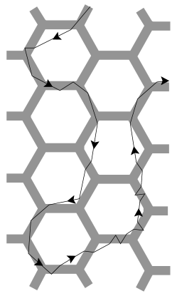
Figure 1: Regular honeycomb foam ($\delta r=0$) and a photon’s random walk in this structure.

We let photons perform a random walk in our model foams by applying the rules of geometrical optics (see Fig. 1). The photons move straight in the liquid or gaseous phase with respective velocities $c/n_{l}$ or $c/n_{g}$ where $c$ is the vacuum speed of light and $n_{l},n_{g}$ are refractive indices. When the photons hit a liquid-gas interface, they are reflected with a probability, also called reflectance, given by Fresnel’s formulas. The respective reflectances for electric polarizations parallel or perpendicular to the plane of incidence are

$$r_{\|}=\left(\frac{\mathrm{tan}(\beta_{l}-\beta_{g})}{\mathrm{tan}(\beta_{l}+\beta_{g})}\right)^{2}\enspace\mathrm{and}\enspace r_{\perp}=\left(\frac{\mathrm{sin}(\beta_{l}-\beta_{g})}{\mathrm{sin}(\beta_{l}+\beta_{g})}\right)^{2}\enspace,$$ (2)

where $\beta_{l}$ and $\beta_{g}$ denote the respective angles of a light ray in the liquid or gaseous phase measured relative to the normal on the interface. They are connected by Snellius’ law: $\mathrm{sin}\beta_{l}/\mathrm{sin}\beta_{g}=n_{g}/n_{l}$. Note that Fresnel’s formulas are symmetric in $\beta_{l}$ and $\beta_{g}$. So the reflectance is the same whether the light ray is hitting the interface coming from the liquid or the gaseous phase. However, there is an important difference: light rays in the optically denser medium ($n_{l}>n_{g}$) experience total reflection for an incident angle $\beta_{l}>\beta^{\ast}=\mathrm{arcsin}(n_{g}/n_{l})$. We stress this point here because it is central for the occurence of photon channelling.

Typically, we launch 10000 photons at one vertex of the underlying Voronoi tesselation in an angular range of $60^{\circ}$ and let them run during a time $t=10^{5}l_{0}/c$. At several times, we calculate the mean square displacement $\sigma^{2}$ from the photon cloud and plot it as a function of $t$. Diffusion constants are then determined from a fit to $\sigma^{2}=4Dt$.

III Photon Channelling

At the core of the observation of photon channelling is the fact that photons can totally be reflected when they hit the liquid-gas interface from the liquid side. Accordingly, a photon spends more time in the liquid phase or, more accurately, the fraction $f$ of the photon’s path that lies in the liquid phase is not equal to the liquid volume fraction $\varepsilon$. Gittings et al measured $f$ with the help of a strongly absorbing liquid and then made a prediction for the two averaged transmission probabilities for photons going from the liquid to the gaseous phase ($T_{l\rightarrow g}$) or the reverse direction ($T_{g\rightarrow l}$). Only in the range $0.04<\epsilon<0.2$, they found that the ratio $T_{l\rightarrow g}/T_{g\rightarrow l}$ deviates from one, indicating photon channelling. Furthermore they gave its approximate value as $T_{l\rightarrow g}/T_{g\rightarrow l}\approx n_{g}/n_{l}$ and also confirmed it by simulations. In the following, we derive this central relation for $T_{l\rightarrow g}/T_{g\rightarrow l}$ analytically, connect it to $f$ and compare it with our simulations.

III.1 Analytic results

We start with defining the averaged transmission probability $T_{l\rightarrow g}$ by

$$T_{l\rightarrow g}=\int_{0}^{\pi/2}p_{l}(\beta_{l})t(\beta_{l},\beta_{g})d\beta_{l}\enspace,$$ (3)

where the angle-dependent transmission coefficient $t(\beta_{l},\beta_{g})=1-r(\beta_{l},\beta_{g})$ is connected to the reflectance $r$ of Fresnel’s formulas introduced in Eq. (2). Note that only the angular range of $\beta_{l}<\beta^{\ast}$ contributes to the integral since $t(\beta_{l},\beta_{g})$ is $0$ for $\beta_{l}>\beta^{\ast}$ due to total reflection. The factor $p_{l}(\beta_{l})$ is the normalised probability of a photon to reach the interface from the liquid side with an incident angle $\beta_{l}$. We write it as

$$p_{l}(\beta_{l})=P_{l}(\beta_{l})/\int_{0}^{\pi/2}P_{l}(\beta_{l})d\beta_{l}\enspace.$$ (4)

Accordingly, we define the transmission probability $T_{g\rightarrow l}$ by

$$T_{g\rightarrow l}=\int_{0}^{\beta^{\ast}}p_{g}(\beta_{l})t(\beta_{l},\beta_{g})d\beta_{l}\enspace,$$ (5)

where we used the symmetry of Fresnel’s formulas with respect to $\beta_{l}\leftrightarrow\beta_{g}$. We still take the angle $\beta_{l}$ for the averaging, therefore the upper limit of the integral is just $\beta^{\ast}$ since photons entering the liquid cannot have a $\beta_{l}$ larger than $\beta^{\ast}$. For $\beta_{l}<\beta^{\ast}$ it makes sense to assume that photons coming from the gaseous into the liquid phase possess the same angular distribution as photons in the liquid, i.e., $P_{g}(\beta_{l})\propto P_{l}(\beta_{l})$. So we write

$$p_{g}(\beta_{l}) = P_{g}(\beta_{l})/\int_{0}^{\beta^{*}}P_{g}(\beta_{l})d\beta_{l}$$ (6)

$$= P_{l}(\beta_{l})/\int_{0}^{\beta^{*}}P_{l}(\beta_{l})d\beta_{l}\enspace.$$

Note again the different upper limit in the integral of the normalization factor compared to Eq. (4). Since $t(\beta_{l},\beta_{g})$ is $0$ for $\beta_{l}>\beta^{\ast}$, the transmission probabilities of Eqs. (3) and (5) appear the same however they differ by the normalization factors of $p_{l}$ and $p_{g}$ in Eqs. (4) and (6) as just mentioned. Therefore the ratio of the averaged transmission probabilities is

$$\frac{T_{l\rightarrow g}}{T_{g\rightarrow l}}=\frac{\int_{0}^{\beta^{*}}P_{l}(\beta_{l})d\beta_{l}}{\int_{0}^{\pi/2}P_{l}(\beta_{l})d\beta_{l}}\enspace.$$ (7)

We now assume that all directions of the photons are equally distributed in the liquid and therefore obtain for the angular distribution of photons reaching the interface, $P_{l}(\beta_{l})=\cos\beta_{l}$. The term $\cos\beta_{l}$ means that the number of photons hitting a given surface area decreases with increasing $\beta_{l}$, i.e., photons approaching the interface on a “shallow” path ($\beta_{l}\rightarrow\pi/2$) have a vanishing probability to hit a given surface area. With $\beta^{\ast}=\mathrm{arcsin}(n_{g}/n_{l})$, the ratio of the mean transmission probabilities becomes immediately

$$\frac{T_{l\rightarrow g}}{T_{g\rightarrow l}}=\frac{\int_{0}^{\beta^{*}}\cos\beta_{l}d\beta_{l}}{\int_{0}^{\pi/2}\cos\beta_{l}d\beta_{l}}=\frac{n_{g}}{n_{l}}\enspace.$$ (8)

This is the result of Gittings et al. Gittings2004 measured in the range $0.04<\epsilon<0.2$ for the liquid fraction. In our simulations we realize $P_{l}(\beta_{l})=\cos\beta_{l}$ by starting the photons in the liquid with a uniform angular distribution. In experiments, photons always enter from the gaseous phase. A fast randomization of the angular distribution in the liquid phase is then achieved by disorder in the foam and by the strong curvature of the interface at the Plateau borders. Such a randomization due to curvature occurs, e.g., in the Sinai billard Sinai .

We now derive how the fraction $f$ of a photon’s path that lies in the liquid phase depends on the liquid volume fraction $\varepsilon$. We assume a stationnary photon distribution in the foam. Then the photon current densities $j_{l\rightarrow g}$ and $j_{g\rightarrow l}$ across an interface have to be equal: $j_{l\rightarrow g}=j_{g\rightarrow l}$. With $j_{l\rightarrow g}=(c/n_{l})\varrho_{l}T_{l\rightarrow g}$ and $j_{g\rightarrow l}=(c/n_{g})\varrho_{g}T_{g\rightarrow l}$, where $\varrho_{i}$ is the number density of the photons in phase $i$, and using relation (8), we find immediately

$$\frac{\varrho_{l}}{\varrho_{g}}=\frac{n_{l}^{2}}{n_{g}^{2}}\enspace.$$ (9)

The ratio of the average times $\tau_{l}$ and $\tau_{g}$ a photon spends in the liquid or gas equals the ratio of the average number of photons in these phases,

$$\frac{\tau_{l}}{\tau_{g}}=\frac{\varrho_{l}V_{l}}{\varrho_{g}V_{g}}\enspace,$$ (10)

where $V_{l}$ and $V_{g}$ denote the respective volumes. To motivate this equation, we consider the average photon number $\varrho_{i}V_{i}$ as a time average over the paths of many photons so that $\tau_{i}\propto\varrho_{i}V_{i}$. In experiments, the average path-length fraction $f=s_{l}/(s_{l}+s_{g})$ is measured. Here $s_{i}$ is the path length in phase $i$. With $s_{i}=(c/n_{i})t_{i}$ and Eqs. (9), (10), we finally obtain

$$f^{-1}=\frac{s_{g}+s_{l}}{s_{l}}=1+\frac{n_{g}}{n_{l}}\left(\frac{1}{\varepsilon}-1\right)$$ (11)

where $\varepsilon=V_{l}/(V_{l}+V_{g})$. With the actual values of $n_{g}=1$ and $n_{l}=1.33$, i.e., $n_{g}/n_{l}=0.75$, we obtain the semi-empirical relation for $f^{-1}$ that Gittings et al. report in Ref. Gittings2004 .

If we do not specify the value of $T_{l\rightarrow g}/T_{g\rightarrow l}$ in the derivation of Eq. (11), we obtain the relation

$$\frac{T_{l\rightarrow g}}{T_{g\rightarrow l}}=\frac{\varepsilon(1-f)}{f(1-\varepsilon)}$$ (12)

that was already given by Gittings et al. Gittings2004 . It links $T_{l\rightarrow g}/T_{g\rightarrow l}$ to the measurable quantity $f$.

III.2 Numeric results

We performed simulations to confirm the analytic results of the previous section always choosing $n_{g}=1$. For $n_{l}=1.33$, we plot in Fig. 2a) the inverse of the path-length fraction $f$ as a function of the liquid fraction $\varepsilon$ which was calculated via Eq. (1) from the channel width $d/l_{0}$. A perfectly ordered model foam and one with disorder $\delta r=0.3l_{0}$ were chosen. The photons were either in the parallel or perpendicular polarization state. The numerical results represented by the symbols agree very well with the analytic prediction of Eq. (11) (full line). Therefore, the diagram and also further simulations clearly show that the validity of Eq. (11) is independent of disorder in the model foam and the polarization state. The dashed line corresponds to $f=\varepsilon$. According to Eq. (11) this means $n_{g}=n_{l}$, i.e., when there is no optical contrast between the cells and the channels. Differently speaking, photon channelling should always occur in this model for $n_{g}\neq n_{l}$. In Fig. 2b), we plot $T_{l\rightarrow g}/T_{g\rightarrow l}$, calculated from Eq. (12), as a function of $\varepsilon$ using the results of Fig. 2a). Again the different numerical data points agree with our theory culminating in Eq. (8) and therefore justify the assumptions made during the derivation of Eq. (8). Finally, we also checked that the effect of photon channelling becomes stronger for increasing $n_{l}$ as expected.

Figure 2: a) Inverse of the path-length fraction $f$ as a function of liquid fraction $\varepsilon$ for a disordered model foam ($\delta r/l_{0}=0.3$) and a perfect honeycomb structure ($\delta r/l_{0}=0.0$). Photons with parallel or perpendicular polarization states are chosen. The full line corresponds to Eq. (11) and the dashed line to $f^{-1}=\varepsilon^{-1}$. Further parameters are $n_{g}=1$ and $n_{l}=1.33$. b) The ratio of the average transmission probabilities $T_{l\rightarrow g}/T_{g\rightarrow l}$ as a function of $\varepsilon$. Otherwise, same description as in a).

IV Photon Diffusion

IV.1 Superdiffusion in Honeycomb Foams

Here we investigate the behavior of photon propagation in the exact honeycomb foam of Fig. 1. In Fig. 3 we plot the mean-square displacement $\sigma^{2}$ of the photon cloud (in units of $l_{0}^{2}$) as a function of time $t$ (in units of $l_{0}/c$) for different refractive indices $n_{l}$ of the liquid phase. The channel-width-to-length ratio is $d/l_{0}=1$. As a reference, the dashed line indicates pure diffusive behavior with $\sigma^{2}\propto t$. Clearly, in the exact honeycomb foam the spreading of the photons is superdiffusive. The effect is strong for short times with an exponent $m$ in $\sigma^{2}\propto t^{m}$ between 1.5 and 1.6. It becomes weaker for large times, e.g., $m=1.1$ for $n_{l}=1.33$. In the framework of Lévy walks, superdiffusion is associated with a distribution of step lengths whose first or second moment (mean value and variance) do not exist Levywalk . When the boundaries of the liquid channels are completely reflecting, photon paths occur that correspond to effective steps of infinite length along the directions of the channels Schmiedeberg05b . In such a system, superdiffusion is most pronounced also for large times as we shall demonstrate in a forthcoming publication Schmiedeberg05b . It becomes weaker by letting the photons enter the gaseous phase since this is a mean to reduce the number of very long or infinite photon steps. Note that in Fig. 3 superdiffusion is less pronounced for smaller $n_{l}$, i.e., when the reflectance at the liquid-gas interface decreases. Another mean to cut long steps would be rounding off the sharp edges in the channel system. Finally, as demonstrated in the next section, introducing disorder in the model foam leads to conventional photon diffusion as observed in experiments.

Figure 3: Exact honeycomb foam: Reduced mean-square displacement $\sigma^{2}/l_{0}^{2}$ of the photon cloud as a function of reduced time $t/(c/l_{0})$ for different refractive indices $n_{l}$ of the liquid phase and for $d/l_{0}=1$. Perpendicular polarization is chosen. The dashed line indicates pure diffusion. Insets: Photon clouds at $t=10^{5}l_{0}/c$ for $n_{l}=1.33$ (top left) and $3.0$ (bottom right).

In Fig. 4, we plot the temporal evolution of the mean-square displacement for different ratios $d/l_{0}$ of channel width to length, the refractive index is $n_{l}=2$. For large ratios such as $d/l_{0}=1$, superdiffusion is stronger since then photons have more possibilities to realize very long effective steps. These steps are visible in the insets that show the photon clouds at time $t=10^{5}l_{0}/c$ for $d/l_{0}=1$ and $10^{-3}$ (see also Fig. 3). The clouds are not spheres as for conventional diffusion, instead, due to the long effective steps, they exhibit peaks along the six equivalent directions of the honeycomb foam. The peaks are more pronounced for stronger superdiffusion.

Figure 4: Exact honeycomb foam: Reduced mean-square displacement $\sigma^{2}/l_{0}^{2}$ of the photon cloud as a function of reduced time $t/(c/l_{0})$ for different ratios $d/l_{0}$. The refractive index is $n=2$ and perpendicular polarization is chosen. The dashed line indicates pure diffusion. Insets: Photon clouds at $t=10^{5}l_{0}/c$ for $d/l_{0}=1$ (top left) and $10^{-3}$ (bottom right).

IV.2 Diffusion in Disordered Voronoi Foams

As soon as we introduce disorder into the Voronoi foam, superdiffusion vanishes and conventional diffusion occurs. This is not unexpected since disorder inhibits long effective steps of a photon as explained in the previous section. In Fig. 5 we plot the diffusion constant $D$, for both parallel and perpendicular polarization of the light wave, as a function of $\delta r$, which quantifies disorder in our Voronoi foams. We expect the diffusion constant to diverge when $\delta r/l_{0}\rightarrow 0$ because of the superdiffusiv behaviour at $\delta r/l_{0}=0$. Our simulations indicate (note the logarithmic scale for $\delta r$) that the divergence is quite weak especially for the perpendicular polarization state. On the whole range of $\delta r$, a clear decrease of the diffusion constant with increasing disorder is visible. We understand this observation since correlations between successive photon steps are destroyed more easily in a disordered foam. Furthermore, the diffusion constant for parallel polarization is larger compared to the perpendicular case due to its smaller reflectance $r_{\|}$, which even becomes zero at the Brewster angle characterized by $\beta_{l}+\beta_{g}=\pi/2$.

Figure 5: Diffusion constant $D$ in units of $l_{0}c$ as a function of disorder $\delta r/l_{0}$ in the model foam with $d/l_{0}=0.1$, $n_{g}=1$ and $n_{l}=1.33$.

Figure 6: Diffusion constant $D$ in units of $l_{0}c$ as a function of the channel width to length ratio $d/l_{0}$ in a disordered model foam with $\delta r/l_{0}=0.3$, $n_{g}=1$ and $n_{l}=1.33$. Symbols indicate numerical results, the lines follow from Eq. (15) derived by a a one-dimensional analytical model.

In Fig. 6 the dependence of the diffusion constant on the channel width to length ratio $d/l_{0}$ is shown for the most disordered foam in our numerical treatment, i.e., for $\delta r/l_{0}=0.3$. The ratio $d/l_{0}$ is directly connected to the liquid fraction $\varepsilon$ via Eq. (1) which offers an explanation for the observed decrease of $D$ with increasing $d$. When the liquid fraction $\varepsilon$ becomes larger, the photons spend more time in the liquid phase where they move with a smaller velocity compared to the gaseous phase. Furthermore, more photons exhibit total reflection at the liquid-gas interface, i.e., photon channelling is more pronounced. Note also that for $d,\varepsilon\rightarrow 0$, the diffusion constant approaches a finite value. This is in clear contrast to experiments durApp and we will comment on it in our conclusions. We have developed a one-dimensional random-walk model which includes a photon-channelling state and whose details are explained in the following section. Its prediction for the diffusion constant (see lines in Fig. 6) gives a remarkable quantitative agreement with the numeric results in Fig. 6. Finally, Fig. 7 demonstrates that the diffusion constant decreases with increasing $n_{l}$. This agrees with intuition since the reflectance increases and the photons in the liquid phase move slower. The random-walk model (see lines in Fig. 7) again gives a good description for the observed behavior with some quantitative deviations for the parallel polarization state.

Figure 7: Diffusion constant $D$ in units of $l_{0}c$ as a function of refractive index $n_{l}$ of the liquid phase in a disordered model foam with $\delta r/l_{0}=0.3$, $d/l_{0}=0.1$ and $n_{l}=1$. Symbols indicate numerical results, the lines follow from Eq. (15) derived by a one-dimensional analytical model.

IV.3 A One-Dimensional Model for Photon Channelling

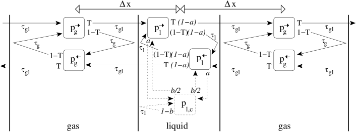
Figure 8: One-dimensional random-walk model in a periodic sequence of gaseous and liquid regions. Five photon states with probabilities $p_{g}^{\rightarrow}$, $p_{g}^{\leftarrow}$, $p_{l}^{\rightarrow}$, $p_{l}^{\leftarrow}$ and $p_{l,c}$ are introduced. The subscript stands for the phase, in which the photon resides, and the superscript arrow for its direction of motion. Photons with angles $\beta_{l}>\beta^{*}$, i.e., photons undergoing total reflection in the liquid phase, are in the photon channelling state with probability $p_{l,c}$. The possible transitions between the states are given by arrows. The transition probabilities and times are explained in the text. Note that the transitions from and into the photon channelling state are instantaneous.

To explain the main features of photon channelling in disordered foams, we have developed a one-dimensional random-walk model. We consider a sequence of gaseous and liquid regions with a lattice constant $\Delta x$, as illustrated in Fig. 8. On a length scale larger than $\Delta x$, we then introduce the coarse-grained probabilities $p_{g}^{\rightarrow}(x,t)$, $p_{g}^{\leftarrow}(x,t)$, $p_{l}^{\rightarrow}(x,t)$ and $p_{l}^{\leftarrow}(x,t)$ for a photon to be at time $t$ at the position $x$ and in a state specified by the indices. Here the lower index means that the photon resides in the gaseous ($g$) or liquid ($l$) phase and the arrow of the upper index gives the direction of motion. All photons are transmitted through the liquid-gas interface with a probability $T$ or they are reflected with a probability $1-T$. In Fig. 8 all possible transitions between the four states are indicated by solid lines, the transmission probabilities are given in non-italic writing. Reflected photons return to their original position, which for concreteness we locate in the middle of each region, after a time $\tau_{g}$ or $\tau_{l}$. Transmitted photons move from the gaseous to the liquid phase or vice versa during the time $\tau_{gl}=(\tau_{g}+\tau_{l})/2$.

So far, all photons can traverse the liquid-gas interface with a probability $T$. To allow for photon channelling in our model, i.e., photons which exhibit total reflection, we introduce a fifth state located in the liquid phase with the probability $p_{l,c}(x,t)$. Within the liquid phase, photons travelling to the right or left switch instantaneously into the photon channelling state with a probability $a$. They return to one of the “moving” states with a probability $b/2$. The numbers $a$ and $b$ are related to each other as we will demonstrate below. With probability $1-b$, a photon in the photon channelling state is reflected at the liquid-gas interface and returns to the same state after the time $\tau_{l}$. All possible transitions connected to photon channelling are indicated by dashed lines in Fig. 8.

The following master equations now quantify all transitions between different photon states:

$$p_{g}^{\rightarrow}(x,t) = (1-T)p_{g}^{\leftarrow}(x,t-\tau_{g})+T(1-a)p_{l}^{\rightarrow}(x-\Delta x,t-\tau_{gl})$$

$$p_{g}^{\leftarrow}(x,t) = (1-T)p_{g}^{\rightarrow}(x,t-\tau_{g})+T(1-a)p_{l}^{\leftarrow}(x+\Delta x,t-\tau_{gl})$$

$$p_{l}^{\rightarrow}(x,t) = Tp_{g}^{\rightarrow}(x-\Delta x,t-\tau_{gl})+(1-T)(1-a)p_{l}^{\leftarrow}(x,t-\tau_{l})+\frac{1}{2}bp_{l,c}(x,t)$$ (13)

$$p_{l}^{\leftarrow}(x,t) = Tp_{g}^{\leftarrow}(x+\Delta x,t-\tau_{gl})+(1-T)(1-a)p_{l}^{\rightarrow}(x,t-\tau_{l})+\frac{1}{2}bp_{l,c}(x,t)$$

$$p_{l,c}(x,t) = ap_{l}^{\rightarrow}(x,t)+ap_{l}^{\leftarrow}(x,t)+(1-b)p_{l,c}(x,t-\tau_{l}).$$

We are interested in the diffusive behavior of the total probability $p(x,t)=p_{g}^{\rightarrow}+p_{g}^{\leftarrow}+p_{l}^{\rightarrow}+p_{l}^{\leftarrow}+p_{l,c}$ that should be visible on large length and time scales. We therefore Fourier transform the master equations (13) and then Taylor expand all the coefficients up to first order in the frequency $\omega$ and up to second order in the wave number $k$. Thus we obtain a set of linear equations:

$$\left(\begin{array}[]{ccccc}-1&(1-T)f(\tau_{g})&T(1-a)g^{-}&0&0\\ (1-T)f(\tau_{g})&-1&0&T(1-a)g^{+}&0\\ Tg^{-}&0&-1&(1-T)(1-a)f(\tau_{l})&b/2\\ 0&Tg^{+}&(1-T)(1-a)f(\tau_{l})&-1&b/2\\ 0&0&a&a&-1+(1-b)f(\tau_{l})\\ \end{array}\right)\left(\begin{array}[]{c}p_{g}^{\rightarrow}(\omega,k)\\ p_{g}^{\leftarrow}(\omega,k)\\ p_{l}^{\rightarrow}(\omega,k)\\ p_{l}^{\leftarrow}(\omega,k)\\ p_{l,c}(\omega,k)\end{array}\right)=0$$ (14)

where $f(\tau)=1-i\omega\tau$ and $g^{\pm}=1-i\omega\tau_{gl}\pm ik\Delta x\pm\omega k\tau_{gl}\Delta x-k^{2}\Delta x^{2}/2$. Now, each probability in Eqs. (14) obeys the same relation, e.g., $\mathrm{det}\mathbf{M}\,\,p_{g}^{\rightarrow}(\omega,k)=0$ where $\mathrm{det}\mathbf{M}$ denotes the determinant of the coefficient matrix in (14). To leading order in $\omega$ and $k$, it reads $\mathrm{det}\mathbf{M}\propto i\omega+Dk^{2}$. Thus, our model indeed reproduces diffusive behavior and gives a formula for the diffusion constant:

$$D=\frac{2\Delta x^{2}bT(1-a)(2-a)}{\left[\tau_{g}b(1-a)+\tau_{l}(a+b-2ab)\right]\left[3aT-2a-4T+4\right]}$$ (15)

(note that $\tau_{gl}=(\tau_{g}+\tau_{l})/2$ was already used).

We now make contact with our two-dimensional model foams. Photons in the four states $p_{g}^{\rightarrow}$, $p_{g}^{\leftarrow}$, $p_{l}^{\rightarrow}$ and $p_{l}^{\leftarrow}$ correspond or lead to photons in the liquid phase whose angle with respect to the interface normal obeys $\beta<\beta^{*}$, i.e., they do not exhibit total reflection. Thus we choose $T=T_{g\rightarrow l}$ where $T_{g\rightarrow l}$ is the average transmission probability introduced in section III.1.

In stationnary equilibrium, the flux of photons into and out of the photon channnelling state has to be equal: $ap_{l}^{\rightarrow}+ap_{l}^{\leftarrow}=bp_{l,c}$. This implies a relation between $a$ and $b$:

$$\frac{a}{b}=\frac{p_{l,c}}{p_{l}^{\rightarrow}+p_{l}^{\leftarrow}}=\frac{\int_{\beta^{*}}^{\pi/2}p(\beta_{l})d\beta_{l}}{\int_{0}^{\beta^{*}}p(\beta_{l})d\beta_{l}}=\frac{n_{l}}{n_{g}}-1\enspace.$$ (16)

Here we have used the formalism of section III.1 to relate $p_{l,c}$ and $p_{l}^{\rightarrow}+p_{l}^{\leftarrow}$ to the probability $p(\beta_{l})$ and then have assumed an equal angular distribution of the photons, thus $p(\beta_{l})\propto\cos(\beta_{l})$, as in section III.1. The quantity $b$ denotes the probability for a photon to leave the photon channelling state. In our two-dimensional model foams this can only occur at a junction where three channels meet since in the channel itself reflections do not change $\beta>\beta^{*}$. The number of reflections necessary to reach a junction scales as $d^{-1}$, we therefore assume $b\propto d/l_{0}$. Since the constant of proportionality is of the order of one, we take $b=d/l_{0}$ to compare the one-dimensional model to the simulation data. In Fig. 6, e.g., variations in $b$ will shift the region where the diffusion constant decreases.

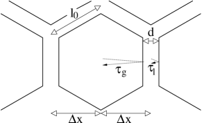
Figure 9: The parameters $\Delta x$, $\tau_{g}$ and $\tau_{l}$ of the one-dimensional photon-channelling model in relation to a two-dimensional model foam: $\Delta x=\sqrt{3}l_{0}/2$, $\tau_{g}=n_{g}(\sqrt{3}l_{0}-d)/c$ and $\tau_{l}=n_{l}d/c$.

The lattice constant $\Delta x$ determines the diffusion constant in the limit where the liquid region tends to zero ($d\rightarrow 0$). From Eq. (15) one finds

$$D(d\rightarrow 0)=\frac{1}{2}\frac{T}{1-T}\Delta x\,c.$$ (17)

In our model foams, $\Delta x$ corresponds to half of the typical bubble size. To compare the diffusion constant of Eq. (15) to our simulation results, we choose $\Delta x$ and the times $\tau_{l}$ and $\tau_{g}$ as shown in Fig. 9, i.e., $\Delta x=\sqrt{3}l_{0}/2$, $\tau_{g}=n_{g}(\sqrt{3}l_{0}-d)/c$ and $\tau_{l}=n_{l}d/c$. As illustrated in Fig. 6 and 7, this gives an excellent agreement with our simulation data. So the one-dimensional model explains the main features of our approach to photon channelling very well. Absolutely crucial for the success of the model is the introduction of the photon-channelling state.

V Conclusions

Photon channelling found in experiments by Gittings et al. is an interesting concept which increases our understanding of the diffusive transport of light in foams. To contribute to its further study, we have simulated the transport of light in two-dimensional Voronoi foams based on ray optics. In perfect honeycomb structures, we find superdiffusive behavior which is connected to the motion of photons in the liquid channels. However, as soon as we introduce disorder into the foams, light transport becomes diffusive. This agrees with our finding that the diffusion constant $D$ only exhibits a weak divergence for decreasing disorder parameter $\delta r$. Furthermore, according to our simulations and in agreement with intuition, $D$ decreases with increasing refractive index $n_{l}$ and also with increasing channel-width-to-length ratio $d/l_{0}$. We are able to model this dependence with the help of a one-dimensional random walk model but only when we introduce a photon-channelling state. Therefore, the importance of photon-channelling becomes evident. The decrease of $D$ with increasing $d/l_{0}$ or liquid fraction $\varepsilon$ is in qualitative agreement with measurements by Vera et al. durApp . However, there is an important difference; whereas Vera et al. observe a divergence of the diffusion constant for $\varepsilon\rightarrow 0$, it assumes a finite value in our simulations and analytic model. The reason is that we consider independent transmission and reflection events at each single liquid-gas interface. If the film thickness becomes sufficiently thin, the effective reflectance and transmittance of thin films seems to be more appropriate, where interference effects are taken into account Miri04 . They lead to a strong decrease of the reflectance for $\varepsilon\rightarrow 0$ and therefore to a divergence of $D$.

Building on the work of Gittings et al. Gittings2004 , we are able to justify their observed relation between the photon’s path-length fraction $f$ in the liquid phase and the liquid fraction $\varepsilon$ without any free parameters. Their further observation that photon channelling only occurs in the region $0.04<\varepsilon<0.2$ will help to improve our understanding of light propagation in foams. For $\varepsilon<0.04$, the extension of the Plateau borders and films are probably too small that pure ray optics is applicable and therefore photon channelling breaks down. In this parameter region, we suggest that the reflectance and transmittance of thin films which include interference effects, as already mentioned in the last paragraph, are the appropriate quantities to model the photons’ random walk. However, we have no understanding why photon channelling ceases for $\varepsilon>0.2$. Especially, our analytic considerations in Sec. III.1 employ very general arguments without relying on a concrete foam structure, so it is not evident why they should break down for larger volume fractions.

Nevertheless, we show in this article that photon channelling in liquid foams can be understood on the basis of ray optics through analytic considerations and simulations using simple model foams. It seems that details of the foam structure are unimportant. We are confident that the results presented in this article add another piece to the puzzle of explaining diffusive light transport in cellular structures such as aqueous foams.

- (1) D. Weaire and S. Hutzler, The Physics of Foams, Oxford University Press, New York (1999).
- (2) D.J. Durian, D.A. Weitz, and D.J. Pine, Science 252, 686 (1991); Phys. Rev. A 44, R7902 (1991).
- (3) J.C. Earnshaw and A.H. Jaafar, Phys. Rev. E 49, 5408 (1994).
- (4) R. Höhler, S. Cohen-Addad, and H. Hoballah, Phys. Rev. Lett. 79, 1154 (1997); S. Cohen-Addad and R. Höhler, Phys. Rev. Lett. 86, 4700 (2001); S. Cohen-Addad, R. Höhler, and Y. Khidas, Phys. Rev. Lett. 93, 028302 (2004).
- (5) A. D. Gopal and D. J. Durian, J. Colloid Interface Sci. 213, 169 (1999).
- (6) M.U. Vera, A. Saint-Jalmes, and D.J. Durian, Applied Optics 40, 4210 (2001).
- (7) G. Maret and P.E. Wolf, Z. Phys. B, 65, 409 (1987); G. Maret, Current Opinion in Colloid & Interface Science 2, 251 (1997); D.J. Pine, D.A. Weitz, P.M. Chaikin, and E. Herbolzheimer, Phys. Rev. Lett. 60 1134 (1988).
- (8) B. A. van Tiggelen, R. Maynard, and A. Heiderich, Phys. Rev. Lett. 77, 639. (1996); H. Stark and T. C. Lubensky, Phys. Rev. Lett. 77, 2229 (1996); B. van Tiggelen and H. Stark, Rev. Mod. Phys. 72, 1017 (2000).
- (9) P.D. Kaplan, A.D. Dinsmore, A.G. Yodh, and D.J. Pine, Phys. Rev. E 50, 4827 (1994).
- (10) A. S. Gittings, R. Bandyopadhyay and D. J. Durian, Europhys. Lett. 65, 414 (2004).
- (11) S. Skipetrov, unpublished (2002).
- (12) MF Miri and H. Stark, Phys. Rev. E 68, 031102 (2003).
- (13) MF Miri and H. Stark, Europhys. Lett. 65, 567 (2004).
- (14) MF Miri and H. Stark, J. Phys. A: Math. Gen. 38, 3743 (2005).
- (15) MF Miri, E. Madadi, and H. Stark, Phys. Rev. E. 72, 031111 (2005).
- (16) M. Schmiedeberg and H. Stark, Superdiffusion in a Honeycomb Billard, in preparation.
- (17) D. Weaire and N. Rivier, Contemp. Phys. 25, 59 (1984).
- (18) A. Okabe, B. Boots, and K. Sugihara, Spatial Tessellations, Concepts and Applications of Voronoi Diagrams, John Wiley & Sons, Chichester (2000).
- (19) L. J. Gibson and F. A. Ashby, Cellular Solids: Structure and Properties, Cambridge University Press, Cambridge (1997).
- (20) H.M. Princen, J. Coll. Int. Sci. 91, 160 (1983); N. Pittet, J. Phys. A: Math. Gen. 32, 4611 (1999); K.Y. Szeto, Xiujun Fu, and W.Y. Tam, Phys. Rev. Lett. 88, 138302 (2002); A.M. Kraynik and D.A. Reinelt, J. Coll. Int. Sci. 181, 511 (1996); Forma 11, 255 (1996); D.A. Reinelt and A.M. Kraynik, J. Coll. Int. Sci. 159, 460 (1996); J. Fluid Mech. 311, 327 (1996); H.X. Zhu, J.F. Knott, and N.J. Mills, J. Mech. Phys. Solids 45, 319 (1997); W.E. Warren and A.M. Kraynik, J. Appl. Mech. 64, 787 (1997).
- (21) J. R. Shewchuk, http://www-2.cs.cmu.edu/quake/triangle.html.
- (22) L. A. Bunimovich and Ya. G. Sinai, Commun. Math. Phys. 78, 247 (1980); 78, 479 (1981).
- (23) G. Zumofen and J. Klafter, Phys. Rev. E 47, 851 (1993).