Multiple scattering suppression in dynamic light scattering based on a digital camera detection scheme

Abstract

We introduce a charge coupled device (CCD) camera based detection scheme in dynamic light scattering that provides information on the single-scattered auto-correlation function even for fairly turbid samples. It is based on the single focused laser beam geometry combined with the selective cross correlation analysis of the scattered light intensity. Using a CCD camera as a multispeckle detector we show how spatial correlations in the intensity pattern can be linked to single and multiple scattering processes. Multiple scattering suppression is then achieved by an efficient cross correlation algorithm working in real time with a temporal resolution down to 0.2 seconds. Our approach allows access to the extensive range of systems that show low-order scattering by selective detection of the singly scattered light. Model experiments on slowly relaxing suspensions of titanium dioxide in glycerol were carried out to establish the validity range of our approach. Successful application of the method is demonstrated up to a scattering coefficient of more than $\mu_{s}=5$ cm^-1 for the sample size of $L=1$ cm.

I INTRODUCTION

Dynamic Light Scattering (DLS) analyzes the intensity fluctuations of light scattered from a medium in the weak scattering limit. This is typically done by means of the normalized intensity autocorrelation function (ACF):

$$g_{2}(q,\tau)=\frac{\langle I(q,t)I(q,t+\tau)\rangle_{t}}{\langle I(q,t)\rangle_{t}^{2}},$$ (1)

where $\langle\cdots\rangle_{t}$ denotes time averaging, $\tau$ is the lag time and $q$ is the scattering wave number or momentum transfer defined by scattering angle $\theta$, the wavelength in vacuum $\lambda$ and the solvent refractive index $n$: $q=4\pi nsin(\theta/2)/\lambda$. The measurable quantity $g_{2}(q,\tau)$ can be linked to actual physical microscopic properties by the normalized field autocorrelation function $g_{1}(q,\tau)$ via the Siegert relation:

$$g_{2}(q,\tau)=1+\beta|g_{1}(q,\tau)|^{2},$$ (2)

where the coefficient $\beta$ depends on the detection optics.

Quite generally the the field autocorrelation function $g_{1}(q,t)$ provides access to thermally driven local dynamic properties on length scales of the order $1/q$. A prominent example is the Brownian motion of colloidal particles in a solvent such as water. For this most simple case the normalized field correlation function can be written as berne:dls :

$$g_{1}(q,\tau)=exp(-D_{0}q^{2}\tau)=exp(-\tau/\tau_{c}),$$ (3)

where $\tau_{c}=1/{Dq^{2}}$ is the relaxation time and $D_{0}$ is the particle diffusion coefficient defined by the Stokes-Einstein relation:

$$D_{0}=\frac{kT}{6\pi\eta R},$$ (4)

with $\eta$ the solvent viscosity, $T$ is the sample temperature and $R$ the particle radius. The equation (3) is widely used in dynamic light scattering for the sizing of small particles.

An essential condition for traditional dynamic light scattering to work is absence of multiple scattering. As soon as higher order scattering becomes considerable (typically if transmission in line-of-sight is lower than 95 per cent) the measured intensity correlation function starts to deviate from the theoretical expectations, leading to a faster decay. Furthermore, information on the scattering wave number as well as on the scattering angle $\theta$ is lost since the detected light is composed of several scattering events with unknown momentum transfer.

The influence of multiple scattering can be reduced by decreasing the concentration of the sample under study or the cell size or by refractive-index matching megen:dynamic . The latter one is usually not possible without changing other sample properties. Limitations to the size of the container are set by the optical quality of the sample cells and by boundary effects. For cylindrical cells minimal diameters of typically $1-3$ mm are used whereas in flat or rectangular containers even smaller photon path lengths are achieved urban:3ddls ; lehner:cells . To maximally reduce the photons path lengths one can use fiber optical probes thomas:fiber directly immersed in the (liquid) sample. This approach known as Fiber Optical Quasi Elastic Light Scattering (FOQELS) has been applied in a number of recent studies (see, e.g. Refs. lilge:fiber ; wiese:fiber ; horn:fiber ). The application of FOQELS is however limited to backscattering angles around 180^∘ and moreover the interpretation of the data is often complicated due to the incomplete suppression of multiple scattering.

Quite a different way of actively dealing with multiple scattering has been put forward over the last two decades. The idea is to carry out two simultaneous DLS experiments with exactly the same scattering vectors in the same scattering volume and analyze the time cross-correlation function. It has been clearly shown that under proper conditions (see Refs.phillies:supp ; phillies:exp ; schatzel:supp ) the cross-correlation function equals the auto-correlation function for single scattering within the range of experimental resolution. Successful implementations of this scheme have been reported by several groups. The techniques are called two color DLS (TCDLS) schatzel:supp ; pusey:suppression and three dimensional DLS (3DDLS) urban:3ddls ; pusey:suppression respectively and the latter one is available commercially lsinstruments .

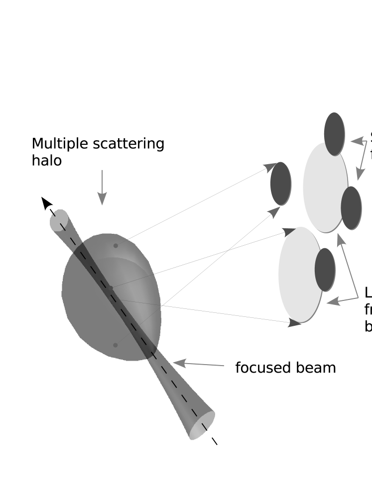
(a)

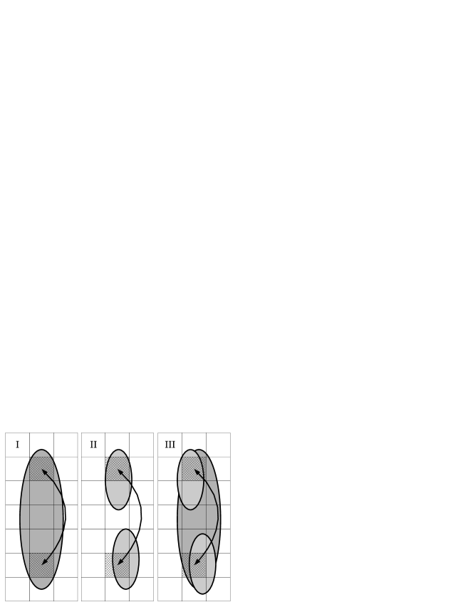
(b)

Figure 1: (a) Illustration of the van Cittert-Zernike theorem: small coherently illuminated areas (such as a focused laser beam) produces large correlated areas (speckles) and and vice versa: large coherence areas (halo from multiple scattering) produces small speckles. (b) Suggested suppression scheme using cross-correlation processing: I) intensity values measured within the same speckle are correlated II) two different speckles are uncorrelated III) for a superposition of small and large speckles intensities detected at a certain distance will be correlated only due to the larger speckles.

Another cross-correlation approach uses a single-beam two-detector configuration  meyer:supp ; schroder:supp . Suppression of multiple scattering is based on a consequence of the van Cittert-Zernike theorem goodman:so , which states that intensity correlations in an observation region are closely related to the Fourier transform of the intensity distribution across the source. This means that a small region of single scattering (e.g. the volume of a focused beam) will produce large correlated areas (speckles), whereas a comparably large halo of multiple scattered photons will give rise to small speckles (see Fig. 1(a)). This is reflected in the well known expression goodman:so for the speckle size $\delta x$ in the far-field geometry: $\delta x=\lambda z/S$, where $z$ is the distance from the light emitting object to the detector and $S$ is the lateral extension of the object along one chosen direction. The consequences for a light scattering cross-correlation experiment are obvious. Spatially resolved detection of the scattered intensity will carry selective information about the spatial distribution of light in the scattering volume.

If we assume that the size of single-scattering volume $S_{1}$ is equal to a average radius of beam cross-section of $S_{1}\approx 20$ µm and the scattering mean free path be $l\approx 1$ mm then the volume of double-scattering extends over roughly a 25 times larger cross section. In practice the dimension of the detected scattering volume will determine $S_{2}$ both for weak and moderate multiple scattering.

Scattered intensities measured in two points separated by distance $\Delta x$

$$\frac{\lambda\cdot z}{S_{1}}\geq\Delta x\gg\frac{\lambda\cdot z}{S_{2}},$$ (5)

will thus be correlated only due to single scattering as shown in the Fig. 1(b) so the normalized intensity cross correlation function (CCF)

$$g^{\Delta x}_{2}(q,\tau)=\frac{\langle I(q,t,0)I(q,t+\tau,\Delta x)\rangle_{t}}{\langle I(q,t,0)\rangle_{t}\langle I(q,t,\Delta x)\rangle_{t}}$$ (6)

will provide the proper estimate of auto correlation function of singly scattered intensity. Such an approach has already been successfully demonstrated by Meyer et al. meyer:supp with the scheme based on cross-correlation of scattered intensities detected by two spatially separated fibers. While the underlying optical background (van Cittert - Zernike theorem) is highly plausible it is more complicated to put forward a detailed theoretical description since this requires modeling of the low order scattering processes. Such treatment has been derived by Lock lock:role for the case of double scattering. He finds the multiple scattering suppression ratio to be approximately proportional to the speckle size ration $S_{2}/S_{1}$ if the detectors are placed at the distance $\Delta x\approx\lambda\cdot z/{S_{1}}$. The suppression ratio can be improved by choosing a larger separation $\Delta x$ albeit at the cost of a decreased signal. Choosing a large distance on the other hand might prove unnecessary for small amounts of multiple scattering. It is due to these practical difficulties, that the technically simpler single-beam cross-correlation geometry is often considered inferior to the two-beam realization (where a sample independent accurate theoretical description is available).

Here we propose an extension of the single-beam cross-correlation method that allows to overcome this shortcoming. Using a charge coupled device (CCD) camera as a detector we can analyze speckle correlations and adapt $\Delta x$ thus assuring single-scattering detection with high accuracy. As we will show this flexibility together with the intrinsically high statistical accuracy of multi-speckle detection leads to a much improved performance of the single-beam two-detector configuration while essentially preserving its technical simplicity.

II EXPERIMENTAL SETUP

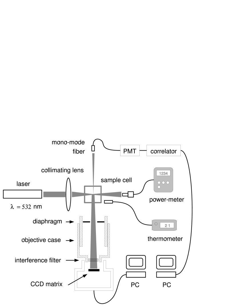
Figure 2: Experimental setup. Light scattered at an angle of 90°  inside the sample cell of thickness $L=1$ cm passes a diaphragm and is collected by a CCD digital camera. In opposite direction light is collected by a mono-mode fiber and a photon counting module to be processed by a hardware correlator. The transmitted collimated intensity is measured to determine the scattering parameters $\mu_{s}$.

The fluctuations of scattered light intensity are monitored in a traditional scattering geometry using a fixed scattering angle. As a light source solid-state laser system (Verdi Coherent Inc., USA) operating at the wavelength $\lambda=532$ nm is used. The beam is strongly focused by a lens with focal length $f=50$ mm inside the sample cell which results in an average beam radius of 20 µm inside the scattering volume. The focal spot was positioned in the center of a rectangular quartz cell (Hellma GmbH, Germany) with inner base dimensions of 10 × 10 mm and height 45 mm. The light scattered from the sample is recorded simultaneously by single-mode fiber connected to a photon counting module (PerkinElmer, Canada) and analyzed with a digital correlator (Correlator.com, USA) from one side and a CCD camera from the opposite side. The CCD grayscale camera “Pixelfly” produced by PCO Computer Optics GmbH, Germany is configured to operate in VGA mode (640 × 480 pixels) with 12 bits resolution and 50 frames per second speed with exposure time $\tau_{0}=20$ ms. This camera is based on a Sony ICX414AL image sensor with the pixel size of 9.9 × 9.9 µm. The dynamic range of analog/digital conversion of the CCD signal is 68.7 dB (according to manufacturer specifications). A diaphragm with an opening diameter of roughly 3.5 mm selects the range of scattering vectors seen by the CCD matrix and also determines the effective scattering volume. The distance for the beam center to the CCD matrix was $z=11$ cm which corresponds to the speckle size of ca. 14 µm or 1.4 pixels.

Scattering angles covered by the CCD chip are found in the range $\theta=90^{\circ}\pm 3.15^{\circ}$. The corresponding scattering vector is equal to $q=(24.59\pm 0.67)\cdot 10^{6}$ m^-1 with a deviation of the order of 2.75 % from the average 90^∘ angle. An improved angular accuracy could be achieved by placing the camera further away from the sample however at the cost of decreased statistical accuracy due to the smaller number of detected speckles. A better way to deal with this problem would be the processing of an angle resolved digital image. However this has not been realized in this study.

In parallel the intensity of the collimated beam transmitted through the cell is measured by a laser power-meter FieldMax (Coherent Inc., USA). The temperature is monitored by a digital thermometer with the probe placed close to the cell surface.

As a model system we studied the Brownian motion of commercial TiO₂ particles in pure (99.5%) glycerol. Solutions were sequentially passed through filters with pore diameters 5 µm and 1.2 µm, respectively. Measurements on samples highly diluted with water reveal a mean hydrodynamic diameter for TiO₂ particles of 293 $\pm$ 15 µm, in qualitative agreement with electron micrographs. For all measurements the temperature was in the range 20 $\pm$ 0.5 ^∘C. Corresponding variations of solvent viscosity are of the order of $\pm$ 5 % handbook:64th . We select Glycerol as a solvent to decrease the particle diffusion coefficient $D_{0}$ and thus enable real-time detection and processing of the scattered intensity fluctuations with a CCD camera .

Typically $10^{4}-10^{5}$ frames were collected corresponding to a measurement time of $15-30$ minutes. The actual number of collected correlation coefficients depends on the processing scheme (see the next section for details) but usually is of the order of $10^{8}$ for the correlation coefficient of smallest delay time.

The turbidity of the sample was characterized by means of the scattering coefficient $\mu_{s}$. It is proportional to the particle density $\rho$ and the scattering cross section $\sigma_{s}$: $\mu_{s}=\rho\sigma_{s}$. Due to the unknown amount of particles lost in the filtering process however no accurate density values are available. Since even fairly small particle densities lead to considerable multiple scattering we can nevertheless safely assume to work in the highly dilute limit. Experimentally $\mu_{s}$ can be estimated from the transmitted intensity $I_{t}$ according to Lambert-Beer’s law for the case of non-absorbing particles: $I_{t}/I_{0}=Aexp(-\mu_{s}L)$, where $I_{0}$ is the intensity incident on the cell, $L$ is the cell thickness, and $A$ describes loss and deflection of intensity at the surface of the cell. The latter is independent of the particle density and was estimated from the transmission coefficient of a cell containing pure glycerol.

III PROCESSING TECHNIQUES

A key element of our study is the optimization of multi-speckle detection and processing schemes. Our goal is to combine intelligent optical realizations with the power of modern parallel processing of a large amount of data acquired by a digital camera. Such optimized data analysis can be both achieved in the time and and the space domain. As the first step we will discuss the application of the multi-tau scheme as developed by Schätzel to our multi-speckle analysis (previous realization for digital cameras are described e.g. cipelletti:ultralow ). Secondly, we will show that a conceptually very similar approach can be used in the space domain in order to improve both the multiple scattering suppression efficiency and the processing speed of our CCD detection scheme.

III.1 Multi-tau correlation scheme

 

(a)

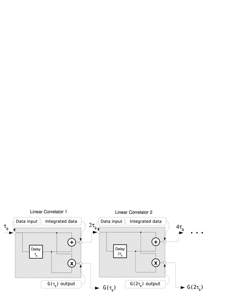
(b)

Figure 3: (a) Principles of the multi-tau correlation scheme. Sequential intensity values $I(t)$ are integrated for the computation of larger lag times.(b) Simplified object scheme to illustrate the cascading of linear correlators used for the realization of the multi-tau correlation scheme.

The multi-tau correlation scheme was originally proposed by Schätzel schatzel:photon to increase the accuracy of hardware correlators for large lag times. In most cases the linear spacing of lag times is not required to analyze single scattering correlation functions. Instead one can increase the distance between lag points in the correlation function for large lag times, thus saving valuable processing time. Such an approach can be easily and efficiently realized with a sequential doubling of the effective exposure time, which furthermore improves statistical accuracy.

Let us suppose that the camera provides data with an initial exposure time equal to $\tau_{0}$ with $1/\tau_{0}$ Hz frequency which implies the absence of delays between the collection of sequential images. Then the doubling of the exposure time to $2\tau_{0}$ can be realized by integrating two sequential values of data obtained with exposure time $\tau_{0}$. In the same way the effective exposure time can be increased to $4\tau_{0}$ and so on as it is shown in Fig. 3(a). From the obtained time series of intensity fluctuations with different exposure times the correlation coefficients can be calculated with a simple linear scale processing.

In terms of software realization this is an ideal case for an object-oriented approach. The main object in this scheme is an Elementary Linear Correlator shown in Fig. 3(b), which receives the sequential data point $I(i)$ as an input at each cycle $i$, multiplies the new value with previous data points $I(i-k)$ for different linearly spaced integer delays $k=0,1,2,...$ and updates the mean values of the corresponding products $\langle I(i)I(i-k)\rangle$. Every second cycle the correlator estimates the mean integrated value of intensity for two sequential time steps $[I(2n)+I(2n+1)]/2$ (where $n=0,1,2,...$) and sends it to the next linear correlator, thus forming a cascading line of correlators. Since the data rate on a sequential correlator is half of the data rate compared to the preceding one, the evaluation period doubles at every correlator. Extra effort has to be taken to optimize the cycles with respect to limitations in computational power.

The elementary correlator unit used in this study was designed to calculate the cross-correlation products together with the auto-correlation. ACF coefficients are calculated on every pixel individually to obtain local values of $\langle I(x,t)I(x,t+\tau)\rangle_{t}$ and $\langle I(x,t)\rangle_{t}$. For the CCF with separation $\Delta x$ we obtain $\langle I(x,t)I(x+\Delta x,t+\tau)\rangle_{t}$ and $\langle I(x,t)\rangle_{t}$ and $\langle I(x+\Delta x,t)\rangle_{t}$. These values are accumulated in each correlator for further spatial averaging.

The scheme described here allows us to evaluate the data in real time and therefore does not set any limitations on the duration of the measurements.

III.2 Binning technique

The low dynamic range of CCD cameras in comparison to photodiodes or photo-multipliers used in previous studies meyer:supp ; schatzel:supp is the main challenge for their utilization in a cross-correlation scheme which requires resolving the small signal from single scattering hidden by a dominating signal from multiple scattering. The problem can be partially solved with an original binning technique developed in the course of this study. If the size of a speckle from single scattering exceeds the area of several pixels it can be approximated with integral values of these pixels intensities. Let us call the bin or meta-pixel the area $S_{x}\times S_{y}$ pixels represented by a single intensity value obtained by integration (or floating-point averaging) of intensities of included pixels. Due to multiple sampling the noise of measurements will be reduced by factor $\sqrt{S_{x}S_{y}}$ dspguide and thus the dynamic range defined as $DR=20\log_{10}SNR$ dB, where $SNR$ is a signal-to-noise ratio, will increase on $10\log_{10}S_{x}S_{y}$ dB. For example for a $10\times 2$ window the dynamic range of our camera model is increased up to 81.7 dB or a $SNR=1.22*10^{4}$. The loss of spatial resolution reduces the statistical accuracy and intercept $\beta$ only if the binning area $\sqrt{S_{x}\times S_{y}}$ is comparable or larger than the coherence area $\sqrt{S_{1}\times S_{2}}$. As a consequence binning leads to partial suppression of multiple scattering by averaging out small speckles. Binning introduces a two-dimensional filtering with a box-like kernel function which will reduce more efficiently the high-frequency spatial fluctuations (multiple scattering speckles) than the lower-frequency fluctuations that are connected to single-scattering speckles. In other words the binning technique in our cross-correlation approach can be considered a spatial analogue of the multi-tau technique in the time domain described above.

III.3 Multi-speckle averaging technique

The ability of cameras to register a large number of independently fluctuating speckles simultaneously can be very efficiently used to increase the statistical accuracy of a measurement by averaging the data along the bins. For the case of independent speckles different pixels or bins can be treated as separate photodetectors and thus their measurements can be processed all together to estimate the correlation function. Actually two possible ways of dealing with this data exist. As it was mentioned above correlators collect the time-averaged products $\langle I(x,t)I(x,t+\tau)\rangle_{t}$ as well as the mean intensity $\langle I(x,t)\rangle_{t}$ for certain bins. Thus the further averaging followed by a normalization with the mean intensity can be performed with products and mean intensities as was proposed in the original multi-speckle scheme kirsch:multispeckle ; knaebel:aging :

$$g^{ad}_{2}(\tau)=\frac{\langle\langle I(x,t)I(x,t+\tau)\rangle_{t}\rangle_{x}}{\langle\langle I(x,t)\rangle_{t}\rangle_{x}^{2}}=\frac{\langle\langle I(x,t)I(x,t+\tau)\rangle_{t}\rangle_{x}}{\overline{I}^{2}},$$ (7)

where $\langle\ldots\rangle_{x}$ denotes the averaging along the entire two-dimensional CCD matrix and $\overline{I}^{2}=\langle\langle I(x,t)I(x,t+\tau)\rangle_{t}\rangle_{x}=\langle\langle I(x,t)I(x,t+\tau)\rangle_{x}\rangle_{t}$ is a mean value of intensity averaged over time and space. This “average-and-divide” sequence can be applied for the ideal case of a uniform illumination of the CCD matrix, i.e. when the mean intensity $\langle I(x,t)\rangle_{t}$ is not a function of $x$. Because for $\tau\rightarrow\infty$, one finds $I(x,t),I(x,t+\tau)\rightarrow\langle I(x,t)\rangle_{t}$ and $\langle I(x,t)I(x,t+\tau)\rangle_{t}\rightarrow\langle I(x,t)\rangle_{t}^{2}$, so for this processing scheme

$$\lim_{\tau\rightarrow\infty}g_{2}(\tau)=\frac{\langle[I(x,t)\rangle_{t}^{2}\rangle_{x}}{\overline{I}^{2}}=\frac{\langle[\langle I(x,t)\rangle_{t}-\overline{I}]^{2}\rangle_{x}}{\overline{I}^{2}}+1=K+1,$$ (8)

where $K=\langle[I(x,t)-\overline{I}]^{2}\rangle_{x}/\overline{I}^{2}$ is the contrast of the picture that would be obtained with infinite exposure time. For the case of uniform illumination $K=0$ due to the fact that $\langle I(x,t)\rangle_{t}=\overline{I}$ all along the detector matrix and thus $g_{2}(\tau\rightarrow\infty)$ will approach 1 so the normalized field autocorrelation function $g^{2}_{1}(\tau)=g_{2}(\tau)-1$ will decay to zero. But even for a slightly non-uniform illumination when $K>0$ the non-zero additive component appears in the measured values $g^{2}_{1}(\tau)$.

To overcome this problem the original multi-speckle scheme was somewhat modified in our study by normalization of the locally estimated correlation coefficients, and averaging only after that (“divide-and-average” sequence):

$$g^{da}_{2}(\tau)=\left\langle\frac{\langle I(x,t)I(x,t+\tau)\rangle_{t}}{\langle I(x,t)\rangle_{t}^{2}}\right\rangle_{x}.$$ (9)

Still this requires the deviation of the mean intensity along the matrix to be small in comparison to the noise level. For a perfectly uniform illumination of the matrix both algorithms provide the same result.

IV RESULTS AND DISCUSSION

We have carried out a series of experiments using samples of different scattering strength, hence different amounts of multiple scattering, ranging from the dilute limit $\mu_{s}L=0.1$ to a regime $\mu_{s}L=5.92$ where the transmitted beam is attenuated to only $0.27\%$ of its initial intensity.

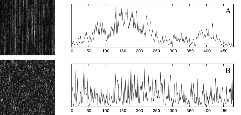
Figure 4: Left: Representative area taken from the recorded images for a weakly scattering (A) and a strongly scattering (B) sample. Right: Spatial intensity fluctuations along the vertical columns of the CCD matrix. Sample A: $\mu_{s}$ = 0.101 cm^-1, estimated speckle size $\delta x$ = 28.02 pixels, sample B: $\mu_{s}$ = 5.92 cm^-1, $\delta x$ = 0.76 pixels

IV.1 Spatial intensity correlations in the speckle pattern

As soon as multiple scattering effects become considerable the detected intensity distribution will consist of a distribution of correlation lengths. The longest correlation length, $\delta x=\lambda z\approx 300$ µm $\approx 30$ pixels can be associated with single scattering whereas higher order scattering leads to smaller speckles. Figure 4 illustrates this by showing the intensity fluctuations along the CCD matrix columns. For the case of single scattering sample ($\mu_{s}$ = 0.1 cm^-1, upper plot) the anisotropy of the speckle pattern can be clearly seen. The reason for the anisotropy is the horizontal confinement of the incident focused beam that defines the scattering volume in this regime. The scale of intensity fluctuations along the “$x$” dimension are of the order of tens of pixels so the correlated areas of intensity or speckles are large. With increasing scattering coefficient $\mu_{s}$ the fluctuations become more pronounced and the correlation length decreases. The horizontal speckle-size is always given by the dimensions of the detected scattering volume both in the single and multiple scattering case.

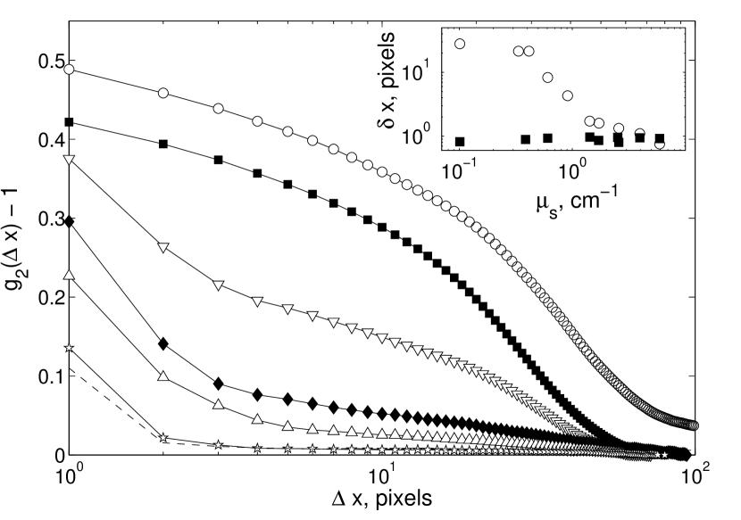
Figure 5: Spatial auto-correlation for different sample turbidities as a function of vertical pixel separation $\Delta x$: ($\circ$) $\mu_{s}$ = 0.10 cm^-1, ($\blacksquare$) $\mu_{s}$ = 0.39 cm^-1, ($\bigtriangledown$) $\mu_{s}$ = 0.88 cm^-1, ($\blacklozenge$) $\mu_{s}$ = 1.43 cm^-1, ($\bigtriangleup$) $\mu_{s}$ = 2.54 cm^-1, ($\star$) $\mu_{s}$ = 5.92 cm^-1. Dashed line ($---$) represents the same estimated in horizontal dimension. Inset shows speckle sizes $\delta x$ ($\circ$) and $\delta y$ ($\blacksquare$) as a function of $\mu_{s}$ for both vertical and horizontal separations respectively. The maximum amplitude of the correlation function is limited to about 0.5 since the speckle size in $y$-direction is comparable to the pixel size

For a quantitative estimation of the actual speckle size the normalized spatial auto-correlation function can be used:

$$g^{s}_{2}(\Delta x)=\frac{\langle I(x)I(x+\Delta x)\rangle_{x,t}}{\langle I(x)\rangle_{x,t}\langle I(x+\Delta x)\rangle_{x,t}},$$ (10)

where $\langle\cdots\rangle_{x,t}$ denotes the time and space averaging. In practice the averaging is performed through all pixel pairs separated vertically by a distance $\Delta x$. A total of 8 independent speckle images is analyzed with an exposure time of 20 ms. Temporal fluctuations are much slower, typically of the order of 0.3 seconds or more, and could thus be neglected. Estimated values for the mean speckle size $\delta x,\delta y$ can be defined by the condition $g^{s}_{2}(\Delta x,\Delta y\ll\delta y)-1=1/e$, $g^{s}_{2}(\Delta x\ll\delta x,\Delta y)-1=1/e$. Since speckles in vertical direction are always small, the limit $\Delta y\ll\delta y$ cannot be reached in our setup and we have thus calculated the correlation length in $\Delta x$ direction using the correlation function normalized with respect to $g_{2}^{s}(\Delta x=1,\Delta y=1)$. Spatial ACFs for samples of various turbidities are shown in Fig. 5 together with the estimated speckle sizes. In vertical direction, with the increase of $\mu_{s}$, the speckle size decreases rapidly. In the multiple scattering limit the speckles are almost isotropic with a size of approximately $1\times 1$ pixels which means that the initially focused beam is dispersed into a diffuse scattering cloud.

The spatial resolution in our experiments allows direct estimation the relative weight of single scattering contributions. For separations much larger than 3 pixels the cross correlation signal will be dominated by single scattering. A separation comparable to the size of a single scattering speckle, $\Delta x\approx 30$ pixels is a good compromise value separating single from multiple scattering.

Note that using a CCD camera we are however not restricted to fixed detector positions as in previous studies. Smaller separations $\Delta x$ could be used in the weak scattering limit whereas a gradual increase of $\Delta x$ in the strong scattering limit simultaneously optimizes multiple scattering suppression and the signal-to-noise ratio.

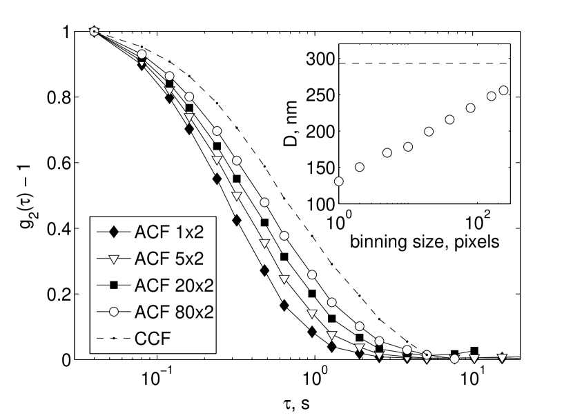
Figure 6: Auto correlation functions obtained with different binning areas together with the cross-correlation function. As the vertical size of the binning area increases the ACF approaches the CCF indicating partial but not sufficient suppression of multiple scattering . The inset shows the estimated particle size ($\circ$) as a function of binning size. The actual size is indicated with by a dashed line.

IV.2 Pixel binning

Instead of pixel by pixel cross correlation we can apply the superior binning approach described before. Proper selection of the binning areas can increase the signal-to-noise ratio and also partially filter out the small multiple scattering speckle. The latter effect is demonstrated in Fig. 6 for different numbers of binning pixels in the vertical direction. Since the horizontal speckle size is constant the binning in this dimension was selected to be 2 pixels.

Auto correlation functions calculated from such larger areas are found increasingly closer to the single scattering function as the binning area is increased. However complete suppression is difficult to achieve since multiple scattering suppression scales linearly with the number of pixels whereas cross correlation scales exponentially with pixel separation. Another disadvantage of very large binning areas is the reduction of the statistical ensemble. Ideally the binning area is chosen somewhat smaller than the size of single scattering speckle in order to retain a high number of independent speckles. In our case the best choice in $x$-direction is in the range of typically 5-20 pixels as it can be seen from Fig. 5.

Figure 7: Correlation functions obtained by different means for an essentially multiple-scattering sample ($\mu_{s}=3.93$ cm^-1). The ACF obtained from the hardware correlator ($---$), the ACF from CCD detection with no binning ($\square$) and the CCF with a separation $\Delta x=40$ pixels ($\circ$) are shown together with the ACF obtained for singly scattering sample ($\bullet$). Inset shows the intercepts for ACF ($\square$) and CCF with separation $\Delta x=40$ ($\bullet$) pixels as functions of $\mu_{s}$.

IV.3 Intensity Correlation Functions

Fig. 7 shows the correlation function for one of the most strongly scattering samples using different measurement schemes. With our optimized cross-correlation ($\Delta x=40$ pixels) and binning approach ($20\times 2$) the measured correlation function perfectly agrees with the single scattering result.

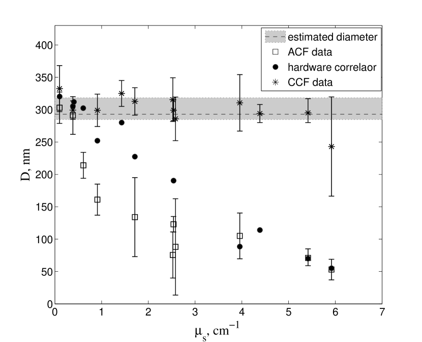
Figure 8: Particle size $D$ determined by different methods as a function of sample turbidity. The CCF diameter remains unchanged up to the limit strong multiple scattering. T. ACF from the hardware correlator ($\bullet$) and from ACF without binning ($\square$) show a rapid decrease as the scattering coefficient $\mu_{s}$ increases.The shaded area indicates the experimental value expected for single scattering (including the uncertainty in particle size and solvent viscosity)

A set of measurements has been carried out and the measured particles diameters are presented in Fig. 8 as a function of scattering coefficient $\mu_{s}$. For the case of dilute samples ($\mu<0.5$ cm^-1) all processing schemes yield the same results within the experimental error. Increasing $\mu_{s}$ results in smaller apparent values of the particle size for the case of autocorrelation measurements (ACF). At the same time the particle diameter obtained using our multiple scattering suppression scheme (CCF processing) stays the same for all $\mu_{s}<5.5$ cm^-1 corresponding to $\mu L=5.5$. Only for the most turbid sample $\mu_{s}\approx 5.92$ cm^-1 a noticeable difference is observed due to the loss of the single scattering signal and the unavoidable increase of error.

Finally we would like to comment on the performance of the multi-speckle averaging scheme implemented in our approach. Neglecting any angular dependence we are treating all $x$-columns equally. As we have seen the size of a single scattering speckle roughly amounts to $30\times 2$ pixels. Since the full CCD chip has $640\times 480$ pixels we detect approximately 5000 independent speckles. This number can be increased only if the diameter of the incident beam is increased, but at the expense of a inferior performance in multiple scattering suppression.

V CONCLUSION AND OUTLOOK

CCD-camera based light scattering can be used to efficiently suppress the undesirable effects of multiple scattering. Our single-beam cross correlation scheme combines for the first time the advantages of multiple-scattering suppression and multi-speckle detection. The latter reduces the collection time for slowly evolving samples dramatically and provides the necessary statistical accuracy to detect even small cross correlation signals deep in the multiple scattering regime. Successful application of these combined processing schemes has been demonstrated for sample turbidities as large as $\mu_{s}L\approx 5$. We think that our relatively simple approach, heavily relying on a flexible processing scheme, can be very useful for a variety of applications for the study of complex fluids and soft materials. With the maximum frame rate available in our experiments the most appropriate areas of application can be found in the field of slowly relaxing systems such as glasses and gels or dense surfactant solutions, to name a few. But at the current rate of development of image sensors and computer hardware much smaller lag times seem to be feasible in a near future. Already now, with the use of modern fast complementary metal-oxide semiconductor cameras with embedded programmable digital signal processors the real-time on-camera calculation of the cross-correlation functions is theoretically possible which in turn would tremendously improve the time resolution.

List of Figure Captions

Fig. 1. (a) Illustration of the van Cittert-Zernike theorem: small coherently illuminated areas (such as a focused laser beam) produces large correlated areas (speckles) and and vice versa: large coherence areas (halo from multiple scattering) produces small speckles. (b) Suggested suppression scheme using cross-correlation processing: I) intensity values measured within the same speckle are correlated II) two different speckles are uncorrelated III) for a superposition of small and large speckles intensities detected at a certain distance will be correlated only due to the larger speckles.

Fig. 2. Experimental setup. Light scattered at an angle of 90°  inside the sample cell of thickness $L=1$ cm passes a diaphragm and is collected by a CCD digital camera. In opposite direction light is collected by a mono-mode fiber and a photon counting module to be processed by a hardware correlator. The transmitted collimated intensity is measured to determine the scattering parameters $\mu_{s}$.

Fig. 3. (a) Principles of the multi-tau correlation scheme. Sequential intensity values $I(t)$ are integrated for the computation of larger lag times.(b) Simplified object scheme to illustrate the cascading of linear correlators used for the realization of the multi-tau correlation scheme.

Fig. 4. Left: Representative area taken from the recorded images for a weakly scattering (A) and a strongly scattering (B) sample. Right: Spatial intensity fluctuations along the vertical columns of the CCD matrix. Sample A: $\mu_{s}$ = 0.101 cm^-1, estimated speckle size $\delta x$ = 28.02 pixels, sample B: $\mu_{s}$ = 5.92 cm^-1, $\delta x$ = 0.76 pixels

Fig. 5. Spatial auto-correlation for different sample turbidities as a function of vertical pixel separation $\Delta x$: ($\circ$) $\mu_{s}$ = 0.10 cm^-1, ($\blacksquare$) $\mu_{s}$ = 0.39 cm^-1, ($\bigtriangledown$) $\mu_{s}$ = 0.88 cm^-1, ($\blacklozenge$) $\mu_{s}$ = 1.43 cm^-1, ($\bigtriangleup$) $\mu_{s}$ = 2.54 cm^-1, ($\star$) $\mu_{s}$ = 5.92 cm^-1. Dashed line ($---$) represents the same estimated in horizontal dimension. Inset shows speckle sizes $\delta x$ ($\circ$) and $\delta y$ ($\blacksquare$) as a function of $\mu_{s}$ for both vertical and horizontal separations respectively. The maximum amplitude of the correlation function is limited to about 0.5 since the speckle size in $y$-direction is comparable to the pixel size

Fig. 6. Auto correlation functions obtained with different binning areas together with the cross-correlation function. As the vertical size of the binning area increases the ACF approaches the CCF indicating partial but not sufficient suppression of multiple scattering . The inset shows the estimated particle size ($\circ$) as a function of binning size. The actual size is indicated with by a dashed line.

Fig. 7. Correlation functions obtained by different means for an essentially multiple-scattering sample ($\mu_{s}=3.93$ cm^-1). The ACF obtained from the hardware correlator ($---$), the ACF from CCD detection with no binning ($\square$) and the CCF with a separation $\Delta x=40$ pixels ($\circ$) are shown together with the ACF obtained for singly scattering sample ($\bullet$). Inset shows the intercepts for ACF ($\square$) and CCF with separation $\Delta x=40$ ($\bullet$)

Fig. 8 Particle size $D$ determined by different methods as a function of sample turbidity. The CCF diameter remains unchanged up to the limit strong multiple scattering. T. ACF from the hardware correlator ($\bullet$) and from ACF without binning ($\square$) show a rapid decrease as the scattering coefficient $\mu_{s}$ increases.The shaded area indicates the experimental value expected for single scattering (including the uncertainty in particle size and solvent viscosity)