The static and dynamic conductivity of warm dense Aluminum and Gold calculated within a density functional approach.

Abstract

The static resistivity of dense Al and Au plsmas are calculated where all the needed inputs are obtained from density functional theory (DFT). This is used as input for a study of the dynamic conductivity. These calculations involve a self-consistent determination of (i) the equation of state (EOS) and the ionization balance, (ii) evaluation of the ion-ion, and ion-electron pair-distribution functions. (iii) Determination of the scattering amplitudes, and finally the conductivity. We present data for for the static resistivity of Al for compressions 0.1-2.0, and in the the temperature range $T$ = 0.1 - 10 eV. Results for Au in the same temperature range and for compressions 0.1-1.0 is also given. In determining the dynamic conductivity for a range of frequencies consistent with standard laser probes, a knowledge of the electronic eigenstates and occupancies of Al- or Au plasma become necessary. They are calculated using a neutral-pseudoatom model. We examine a number of first-principles approaches to the optical conductivity, including many-body perturbation theory, molecular-dynamics evaluations, and simplified time-dependent DFT. The modification to the Drude conductivity that arises from the presence of shallow bound states in typical Al-plasmas is examined and numerical results are given at the level of the Fermi Golden rule and an approximate form of time-dependent DFT.

I Introduction

The static conductivity of matter in the plasma state can be calculated with some confidence, at least for a number of “simple” plasmas, using an entirely first-principles approach per87 ; eos95 . Comparisons with experiments are available for a wide range of conditions, at least for Al plasmas benageR . Another transport property of great interest is the frequency-dependent conductivity $\sigma(\omega)$. Optical probes provide a convenient diagnostic tool for this plasma conductivity, and common laser-probe wavelengths, e.g., 300-800 nm, become the window of interest. In fact, many experiments on laser-plasma interactions related to inertial fusion have concentrated on frequency tripled (with the fundamental $\omega$ at 1$\mu$m from glass lasers) light, $3\omega$, 351nm, while there is also current interest in the $2\omega$ (527 nm) regime as an option for indirect-drive ignitionniemann . Normally, if the probe frequency is less than the plasma frequency, the probe photons fail to enter the material and only weakly ionized systems can be accessed. However, the recent development of extremely thin (”nanoscale”) plasma-slab techniquesng , known as idealized-slab plasmasngcdw has made it possible to study dense plasmas with low-frqeuency probes, both in transmission and in reflectivity.

Density-functional calculations are of two types. The first type depends heavily on quantum MD (QMD) simulations, e.g, Car and Parrinello treat only the electrons via Kohn-Sham theory, while the ion subsystem, explicitly represented by a convenient number $N$ (of the order of $\sim$ 32-256) of ions, is made to evolve in time and an average over millions of configurations is taken. In full Quantum Monte Carlo (QMC) simulationsceperley81 ; kwon , even Kohn-Sham theory is not used and hence full QMC is not practical for typical plasma problems. The second type of DFT is typified by our approach where both electrons and ions are treated by DFT, so that both subsystems are described by two coupled “single-electron” and “single-ion”, Hartree-like Kohn-Sham equations. The many-body effects (i.e, many-electron and many-ion effects) are included through the exchange-correlation or correlation potentials. This allows an enormous simplification in the numerical work involved. These equations may be further reduced to extremely simpilified Thomas-Fermi approaches yielding approximate results for plasma properties which are within an order of magnitude of the more refined results, even in unfavourable casesleemore .

The general optical conductivity problem is essentially the same as that of opacity calculations for warm dense mattergri . However, here we approach it from the static-conductivity ($\omega=0$) regime, and take account of free-free processes as well as shallow bound states which may exist. The static-conductivity provides an evaluation of the dynamic conductivity near $\omega$ = 0 via the basic Drude formula which assumes a constant relaxation time $\tau$, taken to be the static collision time $\tau(0)$. Hence our task can be stated as follows:

1. Calculation of the static resistivity. This involves the following steps:

   1. Calculate the Kohn-Sham atom in an electron gas of density $n$.

   2. Use the Kohn-Sham results to form pseudopotentials $V_{ie}$ and scattering cross sections at the given density $\rho$ and temperature $T$.

   3. Use the $V_{ie}$ to form pair potentials and pair-distribution functions. Here the Kohn-Sham equation for the ion-subsystem can be approximated by some form of the hyper-netted-chain equation (HNC) with bridge terms.

   4. Calculate the EOS, ionization balance etc., to obtain effective ionic charges $\bar{Z}$, electron density $n=\rho/\bar{Z}$etc., and self-consistently, repeating from item (a).

   5. Calculate the static resistivity and the static relaxation time $\tau(0)$ using, e.g, using a Ziman-type formula valid for strong coupling and finite $T$.

2. Use the energy-level structure of the Kohn-Sham atom for the $\rho$ and $T$ regimes of interest to set up bound-bound, or bound-free processes which fall within the range of frequency $\omega$ considered. Corrections may be necessary since the Kohn-Sham theory does not provide good excitation energies.

3. Construct the dynamic conductivity $\sigma^{0}(\omega)$. This yields results equivalent to the Fermi golden rule.

4. Extend the calculation of $\sigma(\omega)$ using time-dependent density-functional theorygri .Include the coupling of electronic transitions to ion-dynamics.

While some aspects of this program can be carried out, it is fair to say that a complete, consistent theory of the transport properties of such many-body systems as posed by warm dense matter, or indeed, even the static properties as embodied in the equation of state for some regimes of density and temperature are open to debate, even for well studied systems like aluminumeosb , and hydrogenhyd . The objective of the present study is to calculate the dynamic conductivity of Al and Au plasmas for a number of compressions and densities where the Drude theory may need correction due to the presence of shallow bound states. Such boundstates ionize when the compression is changed, and produce distinctive changes in transport properties. Sharply rising static resistivities under a change of compression is a common feature of some of the theoretical calculations shown here. However, the establishment of a genuine phase transition requires more careeos95 . The $\sigma(\omega)$ of expanded liquid metals and plasmas showbhat effects arising from clustering and excitonic effects, as the metal-insulator transition is approached. These excitonic effects are not important in dense systems. While Al has been an object of extensive study, recent experiments in the warm dense matter regime have focused on gold targetsjapmore ; aung . Here we present numerical results for Al and Au for several compressions and temperatures.

II static resistivity

We use atomic units (Hartree=1 a.u., the Bohr radius $a_{0}$ = 1, with $|e|=\hbar=m_{e}=1$). The atomic unit of resistivity, given by $\hbar a_{0}/e^{2}$ has a value of 21.74 $\mu\Omega$cm. If the equilibriation of the electron distribution perturbed by the applied electric field is governed by a relaxation time $\tau$, the conductivity $\sigma$ is given as:

$$\sigma=\frac{\omega_{p}^{2}}{4\pi}\,\tau$$ (1)

A mean free path $l_{mfp}$ = $<v>/\tau$, where $<v>$ is some characteristic mean velocity, is often introduced. If electrons were classical point particles, then it is evident that $l_{mpf}$ cannot be smaller than the mean separation between collision centers. This is sometimes called the Joffe-Regel-Mott rule, and holds well in many semiconductors. However, electrons are quantum particles (wave packets) with an extension of the order of the thermal de Broglie length. Further, $\tau$ depends on the electron momentum $k$. Thus there are examples where $l_{mpf}$, obtained by some averaging process, is in fact smaller than some estimated “mean-ion separation”. Although the concept of the mean free path is implicit in the Boltzmann-equation approach, this is not necessary in the Dyson equation which replaces the Boltzmann equation in the quantum case. If the mean free path is large, the “particle picture” of the electron applies, while if this is comparable to the lattice parameter, then we are in the diffraction limit and the wave picture must be used. The Dyson equation, valid at both extremes, describes the one-particle propagator which is closely related to the distribution function appearing in the Boltzmann equation. The derivation of a transport coefficient from the Dyson equation leads us to the current-current correlation function. This is closely related to various two-body distributions and collision kernels found even in classical kinetic models. Unfortunately, although formal expressions can be written down, their evaluation using Green’s functions or related methods becomes impractical, especially if bound states are present. In effect, Green’s-function methods can be pushed to, say, second order in the screened interactions. Such an approach is sufficient if there are no boundstates associated with the scattering potential. Attempts to go further rapidly become intractable and useless.

Our approach is to use a variety of techniques and replace the ion-electron interactions by suitably constructed pseudopotentials, or use scattering cross sections calculated from phase shifts. This requires a fairly sophisticated non-perturbative description of the ion-ion and ion-electron correlations in the plasma.

II.1 Description of the plasma using the Kohn-Sham equations

We begin with the bare nuclei and construct the electronic and ionic structure of the plasma. The interaction of the nucleus with the electron fluid is a highly nonlinear process and attempting to treat it using perturbation theory is unfruitful. Hence we use the Kohn-Sham technique, and construct the non-linear charge density around the nucleus. The nucleus, together with its charge cloud of bound states and continuum-electron states constitute a neutral object. This neutral object is called the neutral pseudo-atom (NPA), following the usage of e.g., Ziman and Dagensdagens . Thus an important result of the Kohn-Sham procedure is the charge-density “pileup”, $n(r)$, around the nucleus that essentially screens the nucleus. A part of this arises from the free electrons and is denoted by $n_{f}(r)$. This $n(r)$ and $n_{f}(r)$ depend on the mean density ${\bar{n}}$ of the electron fluid, temperature $T$, and the nuclear charge $Z$. The Kohn-Sham procedure leading to the NPA provides the phase shifts suffered by the continuum electrons when they scatter from the nuclei. These are used for constructing the scattering cross sections (or pseudopotentials) which describe the electron-ion interaction. The pseudopotential has an effective ionic charge $\bar{Z}$ and it behaves as $-\bar{Z}/r$ for large $r$. The rapid oscillations of the potential near the nucleus is replaced by a weak, smooth core region as the “valence” electrons do not really penetrate the ion-core. The pseudpotentials used in many of the solid-state or molecular code packagescodes have the necessary transferability and could be quite useful. However, they assume that the pseudopotentials would be used within a Schrodinger or Kohn-Sham type procedure rather than in a linear-response scheme, and hence they cannot be directly used within a Ziman-type formula.

Sometimes, instead of using the all-electron Kohn-Sham equation or using a suitably constructed pseudopotential, the electron-ion interaction is replaced by a Yukawa-type interaction (effectively, a Debye-screened interaction). The electronic structure is calculated for such a static-screened nucleus. This procedure is not justifiable since the energies of bound-state electrons correspond to very high frequencies at which there is no screening. Further, the orthogonality of the continuum eigenstates and the bound states ensures that there is very little penetration of the free electrons into the bound-electron region. Consequently, there is very little screening of the inner bound states, where as the Yukawa potential screens the inner bound states as well. Thus calculations using a Debye-like potential in warm dense matter is likely to be incorrect irrespective of whether the Born approximation, or a T-matrix, etc., were used.

In the case of Al and also Au, it is possible to construct, in many situations, a soft pseudopotential $V_{ie}(q)$ which is weak in the sense that it is possible to recreate the non-linear electron-density “pileup” $n_{f}(r)$, obtained via the Kohn-Sham equation, by within linear response theory. That is, we d͡efine the $V_{ie}(q)$ such that

$$n_{f}(r)=-V_{ie}(q)\chi(q)$$ (2)

Here $\chi(q)$ is the electron linear-response function. Unlike the transferable pseuodpotentials used in it ab initio packages, this $V_{ie}(q)$ is specific to the chosen $Z$, $\bar{n}$, $T$, and the atomic number $Z$. It is often convenient to write the pseudopotential in the form

$$V_{ie}(q)=\bar{Z}M_{q}v(q),\;v_{q}=4\pi/q^{2}$$ (3)

where $v_{q}$ is the bare Coulomb potential and $M_{q}$ is a form factor. Only a local pseudopotential is used, and this is quite adequate for an analysis of the experimental data currently available. Since the pseudopotential is weak by construction, the ion-ion pair potential can be taken to be

$$U_{ii}(q)=4\pi\bar{Z}^{2}/q^{2}+|V_{ie}(q)|^{2}\chi(q)$$ (4)

Given $U_{ii}(q)$, the ion-ion distribution function $g_{ii}(r)$ and the structure factor $S(k)$ can be calculated using the Hyper-netted-chain (HNC) equation or its extension where a bridge term is included. We note (see below) that the HNC equation (or its extension) is in fact the Kohn-Sham equation for classical particles ( here, Al^z+ or Au^z+ ions ) for certain choices of the ion-ion correlation potential (there is no exchange potential because the ions are classical particles).

To summarize, by using the Kohn-Sham procedures, we have thus obtained the ion-electron pseudopotential $V_{ie}(q)$, the structure factor $S_{ii}(q)$, and the charge density $n_{ie}(r)$, and an effective ionic charge $\bar{Z}$ which enters into the pseudopotential. The phase shifts have been used to construct a scattering cross sectionper87 which may be used instead of the pseudopotential. Hence we have a completely self-consistent procedure for obtaining all the relevant quantities starting from the nuclear charge of the element. The numerical codes for carrying out these procedures are available via the internet, to any interested researcherweb .

II.2 Is this a “one-center” approach ?

To answer this question, we consider the density-functional theory of a two component system consisting of electrons (density profile $n(r)$ ), and ions, with a density profile $\rho(r)$, with respect to an ion positioned at the originilciacco . Then the Hohenberg-Kohn-Mermin theorem states that the free energy $F[n(r),\rho(r)]$ is a functional of the density distributions such that:

$$\partial F[n(r),n(r)]/\partial n(r) = 0$$ (5)

$$\partial F[n(r),\rho(r)]/\partial\rho(r) = 0.$$ (6)

The first of these equations leads to an effective single-electron equation, viz., the Kohn-Sham equation where the effective potential contains an exchange-correlation potential which takes account of many-electron effects. The second equation also leads to a Kohn-Sham equation which is a classical equation for a single ion. This also contains an ion-ion correlation potential which brings in the effects of the multi-centered system. It can be seen that this classical Kohn-Sham equation reduces to the HNC equation for a certain choice of the ion-correlation potential. Further, for “simple” metallic plasmas like Al where the pseuopotential is weak, this scheme relates closely to pair-potential based liquid-metal theory. Such a simplification does not hold, for e.g., for hydrogen plasmashyd . Since ion-ion, ion-electron and electron-electron correlations are included in the theory, it is not a single-ion model of the plasma. It is firmly rooted in a many-electron, many-ion DFT approach which does not invoke the Born-Oppenheimer approximation. Since the theory is explicitly based on distribution functions, it is manifestly non-local and can be easily implemented to be free of electron self-interaction errors. Our approach may be contrasted with the Car-Parrinello (CP) approach where DFT is used only for the electrons, while the ions are explicitly and individually treated by classical molecular dynamics. CP avoids the need for an ion-correlation potential, but demands a much larger computational effort. Some of these efforts, based on MD methods (e.g, Ref. kwon ; surh ) have confirmed results obtained by the numerically simpler methods that we have used.

II.3 Extended Ziman formula for strongly-coupled electrons and ions.

The Ziman formula is an application of the Boltzmann equation to liquid metals. It was extended to finite temperatures by a number of authors.geoffry The crux of the problem is the evaluation of the collision rate. Compared to some methods well known in plasma theory (e.g, Lenard-Balescu) the collision rate is easily evaluated using the “Fermi golden rule”. In this section we briefly recapitulate Ziman theory in the language of the Fermi golden tule. In the relaxation-time approximation we assume that the perturbed Fermi distribution $f(k)$ for electrons with momentum $\vec{k}$ relaxes towards the equilibrium distribution $f_{0}(k)$ according to the equation:

$$-\frac{\partial f}{\partial t}\big{|}_{col}=\frac{f(k)-f_{0}(k)}{\tau(k)}$$ (7)

Considering an electron scattered elastically from state $\vec{k}$ to state $\vec{k^{\prime}}$, with $|k|=|k^{\prime}|$, $\epsilon_{k}=\epsilon_{k^{\prime}}$, the net scattering rate is the difference of the two processes $(\vec{k}\to\vec{k^{\prime}})-(\vec{k^{\prime}}\to\vec{k})$. The initial and final densities of states for the $\vec{k}\to\vec{k^{\prime}}$ process is $f(k)$ and $[1-f(k^{\prime})]$. Hence the Fermi Golden rule gives

$$R(k\to k^{\prime}) = (2\pi/\hbar)\sum|T_{kk^{\prime}}|^{2}\delta(\epsilon_{k}-\epsilon_{k^{\prime}})f(k)(1-f(k^{\prime})$$

$$R(k^{\prime}\to k) = k k^{\prime}$$ permutation of with etc.,

Since $\epsilon_{k}=\epsilon_{k^{\prime}}$, this involves only an angular integration and $|k|=|k^{\prime}|$. Since the energy is not changed, the static resistivity arises purely from momentum randomization. The change in momentum is $q^{2}=2k(1-cos(\theta))$. Here $\theta$ is the angle between $\vec{k^{\prime}}$ and $\vec{k}$. This $(1-cos(\theta))$ term does not appear in the usual relaxation time which is the time between scattering events. Using these rates in Eq. 7, we obtain a result for the inverse of the relaxation time.

$$\frac{1}{\tau(k)}=2\pi\sum\delta(\epsilon_{k}-\epsilon_{k}^{\prime})|T_{kk^{\prime}}|^{2}(1-cos(\theta))$$ (8)

Here the sum merely indicates the integration over $\theta$. The “$T$-matrix” appearing here describes the scattering of an electron by the whole ion-distribution (i.e, not just one ion). Given a set of ions at instantaneous positions $\vec{R_{I}}$, then the interaction of an electron at $\vec{r}$ with the whole distribution is of the form:

$$V(r)=\sum_{I}V_{ie}(\vec{r}-\vec{R}_{i})$$ (9)

The matrix element between the initial state $\vec{k}$ and the final state $\vec{k^{\prime}}$, with $\vec{q}$ = $\vec{k^{\prime}}-\vec{k}$ is:

$$V(q)=\sum_{I}\bar{Z}M_{q}v_{q}e^{iq\cdot\vec{R_{I}}}.$$ (10)

Note that

$$\rho_{q} = \sum_{I}exp(i\vec{q}\cdot\vec{R_{I}})$$ (11)

$$<\rho_{q}\rho_{-q}> = N_{i}S_{ii}(q).$$ (12)

Thus the ion-ion structure factor $S(q)$ and the single-ion scattering cross section (or the pseudopotential) from a single ion combine to give the full scattering $T$-matrix. The dependence on the structure factor becomes negligible for $T>10$ eV. The individual scattering cross section can be replaced by a single-center $T$-matrix (to be denoted by $t_{kk^{\prime}}$) obtained from the phase shifts of the NPA calculation for a single nucleus. The $S(q)$ is also obtained from the pair-potential constructed from the same NPA calculation. In Ref. per87 we showed how to avoid the calculation of the $S(q)$ by directly computing the scattering cross section from the whole ion distribution. That is, $T_{kk^{\prime}}$ s not factored into single-center $t_{kk^{\prime}}$ and the associated structure factor. Such an approach is needed for strongly interacting systems where such a factorization may not be valid. In this context we note that the resistivities calculated by us using the ”single-center” model (ie., $t_{kk^{\prime}}S(q))$, and the full ion-distribution model ( $T_{kk^{\prime}}$ for strong-scattering) for H-plasmas were independently confirmed by the quantum Monte Carlo simulations of Kwon et alkwon . However, if the pseudopotential is weak, the $S(k)$ and the single-center $t(k)$ may be used.

Given the inverse relaxation time $1/\tau(k)$ for an electron of momentum $k$, or equivalently, $1/\tau(\epsilon)$ for the energy, $\epsilon=k^{2}/2$, we need to average this over all electron energies to obtain a resistivity or a conductivity. The averaging used in the Ziman formula leads to a resistivity, while a direct application of the Boltzmann equation would lead to a conductivity. Thus,

$$\sigma=\frac{\omega^{2}_{p}}{4\pi}<\tau(\epsilon)>,\;\;R=\frac{4\pi}{\omega^{2}_{p}}<1/\tau(\epsilon)>$$ (13)

The Boltzmann equation shows that the averaging relevant to the conductivity calculation is such that

$$\sigma=\frac{\omega^{2}_{p}}{4\pi}\frac{2}{3n_{e}}\int\frac{d\epsilon}{\pi^{2}}(\surd{2}\epsilon^{3/2})\frac{-\partial f_{0}(\epsilon)}{\partial\epsilon}\tau(\epsilon)$$ (14)

On the other hand, the averaging over the $1/\tau(\epsilon)$ used in the extended Ziman formula for the resistivity is somewhat different.

$$<1/\tau>=-\int_{0}^{\infty}d\epsilon g(\epsilon)\frac{\partial f(\epsilon)}{\partial\epsilon}\tau(\epsilon)^{-1}$$ (15)

Here $g(\epsilon)$ is a density-of states factor which is unity for free non-interacting electrons. It should be constructed from the phase shifts in a strongly scattering environment.

The initial assumption, Eq. 7, was that the modified distribution was defined via a relaxation time. A more complete approach is to represent the modified part $\delta f(k)$ as a series expansion in a set of suitably constructed orthogonal polynomials, and obtain a variational solution. The set of polynomials appropriate for degenerate (and partially degenerate) electrons has been discussed by Allen.allenpoly . In the classical limit, such polynomials are the well known Sonine polynomials. The usual relaxation-type approach is equivalent to a single-polynomial solution. This is adequate for dense Al-plasmas, and for the range $0<T<10$ eV studied here. However, this is probably not so for Al at 1/4 of the normal density, or for lower densities. We have less experience with Au-plasmas to assess the quality of the resistivities for Au obtaind here.

II.4 Numerical results in the static limit.

The static resistivities for Al calculated using the above methods (and some extensions of it) have been compared with experiment by Benage et al.benageR Given the uncertainties in the experiment and the various approximations in the theory, the agreement is quite good. However, there are a number of difficulties in the calculation. If we consider an Al-plasma at a compression $\kappa$=0.25, at $T>2.5$ eV the Al-ion has the bound shells $1s,2s,2p$, and $3s$. The $3s$ level becomes increasingly shallow as the temperature is reduced. Below approximately $T\sim 2.5$ eV, the $3s$ level begins to “evaporate” and becomes free, i.e, the $3s$ bound electrons ionize. Even at 2.5 eV, the occupation of the $3s$ level is $\sim$ 0.744. The ionization state $\bar{Z}$ increases from $\sim 1.667$ to 3. The model where we have a single average $\bar{Z}$ is clearly not satisfactory in such a region. The plasma contains an equilibrium mixture of several ionization states $\bar{Z_{i}}$ with concentrations $x_{i}$ such that

$$\bar{Z}=\Sigma_{i}x_{i}\bar{Z_{i}}$$ (16)

For such situations (and indeed in general), the concentrations $x_{i}$ have to be determined from the minimum of the total free energy. If $n$ species of ions are possible, then $n$ different Kohn-Sham equations have to be solved, and $n(n+1)/2$ ion-ion distribution functions have to be determined, and the total free energy has to be calculated as a function of $n$ and $x_{i}$. The minimum property of the free energy yields the equilibrium plasma conditions from which the resistivity is calculated, using the $n$ scattering cross sections and the $n(n+1)/2$ structure factors. We reported such a calculation for $Al$ in Ref. eos95 . Our experience is that, even with a multi-ion fluid model, the self-consistent equations may fail to converge since the $3s$ level (or the $2p$ level) affects the iterative procedure. Majumdar and Kohn have shown that physical properties of a system should be continuous across the region where an electronic state moves from being a bound state to a continuum statemajum . Hence we may calculate the resistivity in two adjacent regions separated by a non-convergent region, and smoothly join the calculated resistivity across the “difficult” region. In Table 2 we show the Kohn-Sham eigenvalues of the bound-electron states for Al ions in various plasmas. Although the Kohn-Sham eigenvalues do not exactly correspond to the excitation energies, they provide an initial estimate which can be improved using the methods of time-dependent density functional theory, or using self-energy calculationsdyson-mott .  

Table 1: Resistivity (in $\mu$ohm cm) of Al plsamsa as a function of the compression $\kappa$ and the temperature in eV, calculated within the approach described in the text.

T$\downarrow\;\;\;\kappa\to$	0.1	0.25	0.5	1.0	2.0	4.0
0.10	1620	801	77	28	38	48
0.25	1582	812	84.1	30.5	37.4	47.0
0.50	1527	847	92.1	34.4	35.8	45.6
0.75	1447	859	99.7	36.7	34.5	45.0
1.00	1340	846	107	38.7	34.5	44.8
1.75	1063	707	122	44.4	34.2	44.6
2.50	844	597	135	50.2	35.4	44.7
3.75	1196	448	148	60.4	39.5	46.0
5.00	916	434	160	70.8	45.1	48.3
7.50	646	380	180	90.6	57.7	54.7
10.0	544	379	194	108.	70.1	61.8

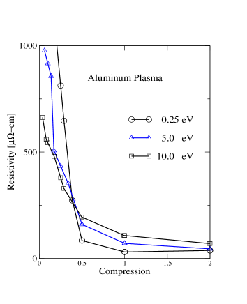
Figure 1: Resistivity of warm dense Aluminum as a function of the compression for several temperatures

Table 2: Kohn-Sham energy-level structure for several $Al$-plasmas within the NPA averag-configuration model

Level	$\kappa=4$	$\kappa=2$	$\kappa=1$	$\kappa=0.5$	$\kappa=0.25$	$\kappa=0.1$
	T=10
$\bar{Z}$	3.043	3.0166	3.0164	3.0194	2.6060	2.2427
2s	-5.7016	-6.3615	-6.9213	-7.4089	-7.9601	-8.5825
2p	-2.9311	-3.5922	-4.1529	-4.6411	-5.1928	-5.8159
3s	–	–	–	–	-0.1871	-0.6168
3p	–	–	–	–	–	-0.1643
	T=2.5
$\bar{Z}$	3.0427	3.0051	3.0003	3.0000	1.6643	1.6240
2s	-5.5247	-6.1819	-6.6655	-7.0257	-7.4435	-7.6634
2p	-2.7838	-3.4422	-3.9268	-4.2875	-4.7055	-4.9258
3s	–	–	–	–	-0.1178	-0.2758
	T=0.1
$\bar{Z}$	3.0437	3.0053	3.0003	3.0000	does not	does not
2s	-5.4903	-6.1444	-6.6282	-6.9811	converge	converge
2p	-2.7462	-3.4008	-3.8853	-4.2393	due to	due to
3s	–	–	–		3s level	3s level

As the density decreases and the temperature increases, we inevitably pass through regions of $T$, $\kappa$ where the problem of bound states which hover near ionization becomes important. We return to this question in discussing the dynamic conductivity of Al-plasma at $\kappa$ = 0.25, and 0.1.

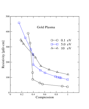
Figure 2: Resistivity of warm dense gold as a function of the compression for several temperatures

Table I shows that, for $\kappa$ = 0.1 the resistivity essentially decreases with $T$, while for $\kappa$ = 0.25 the resistivity gradually increases in value, goes through a plateau-like region, and then begins to decrease with temperature. The same behaviour holds for the other higher compressions, but the table given here does not go high enough in temperature (for the higher densities) to show the plateau effect and the onset of the decrease of $R$. Some authors have interpretted the plateau in the resistivity as indicating a situation where the mean-free path has become as small as possible ( as in the Joffe-Regel rule). We disagree with this explanation of the existence of a resistivity plateau in these cases in terms of a saturation of the mean-free path. Quantitative agreement is provided with a very different picture of what happens in the plasma. As the material is heated, its resistivity increases just as in a metal, due to the increased availability of a strip of states (of width $k_{B}T$) at the Fermi surface for the “phonon-like” scattering to take place. However, as $k_{B}T$ increases, the number of current carrying electrons also increases, compensating the resistivity increase. During this process the chemical potential $\mu$ of the plasma electrons begins to decrease, and a temperature $T_{\mu=0}$ is reached when $\mu$ passes through zero and towards negative values. Then the Fermi sphere is gets broken down and from then on, all the electrons, and not just those near the Fermi surface, begin to conduct. The plasma is essentially classical. The resistivity decreases as the temperature increases. We are in fact in the Spitzer-like regime. The plateau defines the transition to the Spitzer-like regime. The Fermi energy of the $\kappa$ = 0.1 case is small and it is already behaving like a classical plasma. In reality the picture is more complicated since the Fermi surface changes not only because of the temperature, but also because the ionization of bound electrons changes the value of $\bar{Z}$. This pushes the value of $T_{\mu=0}$, and the onset of the plateau to higher temperatures than in a model with constant $\bar{Z}$. It is easy to allow for this in a calculation of $T_{\mu=0}$ and confirm that the resistivity $R(T,\kappa)$ given in our table (and in Ref.milsch ) is consistent with this picture.

II.5 Contribution to the resistivity from electron-electron scattering.

Discussions of the electrical resistivity of plasmas sometimes contain allusions to the e-e contribution to the electrical resistivity. However, the electron-current operator $\vec{j}=(e/m)\vec{k}$ commutes with the electron-electron interaction Hamiltonian $H_{ee}$.

$$\vec{j}H_{ee}-H_{ee}\vec{j}=0$$ (17)

This shows that the current is conserved under the e-e interaction. Hence electron-electron interactions cannot contribute to the resistivity arising from the electron current. However, the e-e interaction has an indirect effect since it screens the electron-ion pseudopotential $V_{e-i}(q)$. That is, electron-ion vertices must occur in all diagrams which contribute to the resistivity. In perturbation-theory approaches to the conductivity or resistivity, it is quite easy to get a contribution to $R$ from e-e scattering alone, if the theory is carried out only to, say, second order. This means, if an all-oder calculation were done, the higher order corrections would exactly cancel the low-oder result for the e-e scattering contribution. Electron-electron interactions contribute to the resistivity of solids where the periodic potential generates Umkapp scattering. But this is not the case in plasmas if they can be considered uniform to within a length scale significantly larger than the mean free path. Classical transport calculations for systems with gradients (i.e, no translational invariance) is well knownmatt . The quantum calculation is also well known in transport across heterostructureslanbut .

III Dynamic conductivity.

If we apply a field $\vec{E}\,cos(\omega t)$ to the system, say using a light probe of frequency $\omega$, then the polarization of the medium is described by the polarization function $\Pi(q,\omega)$ which is directly connected with the transverse dielectric function $\varepsilon(\omega)$ and the dynamic conductivity $\sigma(\omega)$. The wavevector $q$ of the photon is nearly zero and may usually be omitted. The real part $\sigma_{r}$=$\Re\sigma(\omega)$ at $\omega\to 0$ reduces to the static conductivity $\sigma$ that was already discussed.

$$\varepsilon(\omega) = 1-\frac{\omega^{2}_{p}}{\omega^{2}}-\frac{4\pi}{\omega^{2}}\Pi(\omega)$$ (18)

$$\sigma(\omega) = i\frac{\omega^{2}_{p}}{4\pi\omega^{2}}+i\frac{\Pi(\omega)}{\omega}$$ (19)

If the effect of interactions and bound states is small, the conductivity of ”free” electrons driven by the field $E_{0}exp(i\omega t)$, and damped by scatterng at ion centers is well approximated by the Drude model. It uses a relaxation time $\tau_{0}$, (or a damping parameter $\gamma_{0}$) independent of the frequency. In partially ionized systems, or when there are interband effects in solids, it is necessary to include bound-free and bound-bond contributions to $\sigma(\omega)$. A useful practical form is the extension of the Drude model where a model dielectric function is used. Thus,

$$\varepsilon(\omega) = \varepsilon_{r}+i\varepsilon_{i}$$ (20)

$$= 1-\frac{\omega^{2}_{p0}}{\omega(\omega+i\gamma_{0})}-\sum^{\lambda_{m}}_{\lambda=1}\frac{\omega^{2}_{p\lambda}}{\omega(\omega+i\gamma_{\lambda})-\epsilon_{\lambda}}$$ (21)

$$\sigma_{r}(\omega) = \frac{\omega\varepsilon_{i}(\omega)}{4\pi}$$ (22)

Here the pure free-electron Drude term uses the damping parameter $\gamma_{0}$ and a plasma frequency $\omega_{p0}$, while other processes are modeled by a finite set of oscillators parametrized by $\gamma_{\lambda}$ and $\omega_{p\lambda}$. This is a form useful for fitting experimental data since reflection and transmission experiments could be used to extract best fit values of $\gamma_{\lambda}$,$\omega_{p\lambda}$, subject to the sum rule (f-sum rule):

$$\int_{0}^{\infty}d\omega\sigma_{r}(\omega)=\frac{1}{4}\sum^{\lambda_{m}}_{\lambda=0}\omega_{p\lambda}=\pi n_{tot}e^{2}/m_{e}$$ (23)

Here $n_{tot}$ involves the free electrons (given by the average charge $\bar{Z}$) as well as the electrons occupying the localized atomic states participating in the optical transitions. Unlike in liquid-metal studies, these are not readily available for warm dense partially degenerate plasmas. Further, the electron populations in the bound and free states are linked by the Fermi distribution associated with the electron temperature and the chemical potential. Hence this LTE (local thermodynmaic equilibrium) type constraint also should be imposed in fitting the experimental data to the model dielectric function. Thus the most fruitful approach is to use the values of the mean ionization $\bar{Z}$, occupation numbers, electron chemical potential $\mu_{e}$, $\gamma_{\lambda}$, $\epsilon_{\lambda}$ etc., provided from the density-functional NPA calculation in setting up the fitting process. The simple Drude equation with a fixed value of $\gamma_{0}$ satisfies the f-sum rule. It can be shown that if we define $\Pi(\omega)$ in terms of the non-interacting polarizability $\Pi^{0}(\omega)$, by the form:

$$\Pi(\omega)=\Pi^{0}(\omega)/[1+G(\omega)\Pi^{0}(\omega)]$$ (24)

where $G(\omega)$ is called a “local-field” correction, then the sum rule is satisfied if it holds for $\Pi^{0}(\omega)$. Thus, if $\Pi(\omega)$ can be calculated, then we can calculate the dynamic conductivity from it.

The effect of corrections to the simple Drude term arising from interband terms in solid Aluminum, were examined many years ago by Dresselhaus, Harrison, and by Ashcroft and Sturm.ash-sturm . They showed that there are band to band transitions near $\sim$.05 and 0.15 of the Fermi energy $E_{F}$ (which is $\sim 12$ eV. for normal density $Al$). The optical conductivity of normal-density liquid Al slightly above the melting point has been measured by Millermiller and shows a simple Drude form. A discussion of liquid metal data including Cu, Ag and Au is found in Faberfaber . The deviations from the Drude form seen in solid-Al arise from the splitting of degenerate bands due to the crystal potential, and to normal interband transitions. Benedict et al. have argued that the thermal broadening of the electron self-energy is by itself sufficient to “wash out” these solid-state effects, even if the ion lattice remained intactbenedict , as may be the case in short-pulse laser generated plasmas. The effect of electron-electron as well as ion-electron interactions on the electron self-energy at finite-$T$ was also discussed by us for the hydrogenic casedyson-mott

When we consider warm dense $Al$-plasmas, the Kohn-Sham eigenvalues can be used to assess if the driving field $\omega$ could excite bond-bound or bound-free processes. As seen from Table 2, the $2s$ levels for the compressed systems ($\kappa$ =0.1, 0.5, 1, 2, 4) occur between -7.4 au to -5.5 au., while the $2p$ level ranges from -4.6 au. to -2.7 au. Hence, the Drude formula would be reasonable for these systems and for standard optical probes. The situation is quite different for the $\kappa$ =0.25 case. Here the $2p$ level ranges from $\sim$ -4.5 au. to -5.5 au., but the $3s$ level is very close to the ionization threshold. At $T$ = 8 eV, the $3s$ level is at -0.165 au, and rises to -0.105 au. near $T$= 3 eV, and then completely disappears for $T$ below $\sim$  2.5 eV. Since a 300-400 nm optical probes corresponds to about 4-3 eV, it is clear that such probes would show deviations from the Drude conductivity for the $\kappa$ =0.25 case. When we go to low temperatures, the $\bar{z}=3$ ionization is very stable, while the $3s$ level creates the presence of $\bar{z}=1,2$ ionization states. In the case of $\kappa$ = 0.1, we have two shallow states , viz., $3s$ and $3p$. The conductivity derived from the model dielectric function, i.e., Eq. 20 would be relevant to the representation of experimental data for such systems. In the following we look at first-principles calculations.

III.1 Perturbational approach to the dynamic conductivity.

In a theory of $\sigma(\omega)$ we are in effect looking for the polarization function $\Pi(\omega)$. If the potential $V_{ie}(q)$ is weak, (no bound states) diagrammatic methods can be used. However, the second-order expression in the screened interaction is essentially the only one that is tractable for realistic potentials. A number of such quasi-second order results exist in the literature, derived using various methods. An old result, due to Hopfield, holds if the structure factor is essentially unityhopfield .

$$\Re\sigma(\omega)=-\frac{\omega_{p}^{2}}{(4\pi\omega)^{2}}\int\frac{d\vec{q}}{(2\pi)^{3}}q^{2}q_{z}|V_{ie}(q)|^{2}\Im[\frac{1}{\varepsilon(q,\omega)}]$$ (25)

A more complete result, including the contribution from the dynamic structure factor of the ions can be written down, using an approach similar to that given by Mahan for phonons.mahan Rŏpke et al. have also discussed second-order expressions within the Zubarev approach which is most suitable for short-ranged potentials free of bound states.ropke The approach used by Mahan is more interesting and may be used for long-range potentials. In fact, even in the two-temperature case where the ions are at a temperature $T_{i}$, while the electrons are at a temperature $T_{e}$, it is easy to show using the Keldysh technique (assuming that the probe frequency $\omega$ does not overlap with core transitions) that the frequency dependent collisional relaxation time $\tau(\omega)$ ismilsch ,

$$\tau^{-1}(\omega)=-(\omega^{2}_{p}\omega)^{-1}\int\frac{q^{2}dqM^{2}_{q}}{(2\pi)^{3}}q_{z}^{2}\int\frac{d\nu}{2\pi}$$ ⋅

$$\Im[\chi_{ii}(q,\nu)]\Im[\chi_{ee}(q,\nu+\omega)]\Delta N(T_{e},T_{i},\nu,\omega)$$

where we have set

$$\Delta N(T_{e},T_{i},\nu,\omega)=[N\{\beta_{e}(\nu+\omega)\}-N\{\beta_{i}(\nu)\}].$$ (27)

Here $N\{\beta_{i}(\nu)\}$ is a Bose factor giving the occupation number of density-fluctuation modes at the temperature $T_{i}$ and energy $\nu$. For the equilibrium situation we simply set $T_{i}=T_{e}$. Then, as $\omega\to 0$, this equation can be shown to reduce to the inverse collision time used in the Ziman formula. In Eq. III.1 the electron response $\chi_{ee}$ and the ion-response $\chi_{ii}$ mediate the energy and momentum exchange between the two subsystems. The imaginary parts of the response functions are related to the dynamic structure factors by a relation of the form:

$$S(k,\omega)=-\frac{1}{2\pi}\coth\big{[}\frac{\omega}{2T}\big{]}\Im\chi(k,\omega)$$ (28)

In the case of the electrons, $\chi(k,\omega)$ can be written down in terms of the Lindhard function $\chi^{0}(k,\omega)$ and the local-field correction $G(k,\omega)$. In the limit where the electrons becomes classical, the Lindhard function simply reduces to the Vaslov function. The dynamic structure factor of the ions can also be modeled in a similar fashion.elr Clearly, if the probe frequency $\omega$ is smaller than the electron plasma frequency, then we may make a static approximation for $G(k,\omega)$. Since normal-density Al (and even Au, depending on the compression) have high plasma frequencies, this is a good approximation for dense Al or Au. However, the static $G(k,\omega=0)$ used should be such that at least the compressibility sum rule is satisfied. Also, we can introduce an $\omega$ dependent model $G(k,\omega)$ with $G(k,\omega)$= $G(k,\omega=0)$ for $\omega<\omega_{P}$, and $G(k,\omega)$ fitted to the high-frequency moment sum rules for $\omega>\omega_{P}$. In practice it is not known how to satisfy all the sum rules. The static pair-distribution function $g(r)$ recovered from the imaginary part of such a response function should also agree with the known $g(r)$ of the electrons at that density. The successful calculation of the $g(r)$, $S(k)$, and the $G(k)$ in a consistent manner for electrons at strong-coupling and arbitrary temperatures (i.e, arbitrary degeneracies) was presented recently in Ref. chncT

Although an extension of the above equation to take account of bound-free and bound-bound electron processes can be written down “by hand”, it is not easy to provide a systematic development. More fruitful approaches are to use density-functional molecular-dynamics simulations or time-dependent density functional theory. We consider these below.

III.2 Conductivity via the Kubo-Greenwood formula and molecular dynamics.

Another approach to the conductivity $\sigma(\omega)$ is to use molecular dynamics to develop the ionic-liquid structure, while retaining a DFT approach only for the electronic structuresilv1 ; alavi ; gillan . The ion subsystem is modeled with, say, typically 32-256 atoms in a simulation box of volume $V_{b}$ which is periodically repeated. An externally constructed pseudopotential is used and an ionization model is assumed. The required number of electrons based on the ionization model is placed in the box. The ions are held at some fixed ionic configuration {$R_{i}$} and the Kohn-Sham electronic wavefunctions $\psi_{f}(r,\{R_{i}\})$ and energies $\epsilon_{f}$ are computed. Given the size of the system, it is not practical to do more than a few k-points; usually only one $k$-point, e.g., the $\Gamma$ point is computed. The conductivity for the given configuration, and for the selected $k$ point with weight $W(k,\{R_{i}\})$ is estimated using the second-order Fermi golden rule formula.

$$\sigma(\omega,\{R_{i}\},k) = \frac{2\pi}{3V_{b}\omega}\sum_{fg}|W(R_{i},k)<\psi_{f}|\vec{p}|\psi_{g}>|^{2}$$

$$(n_{f}(k)-n_{g}(k))\delta(\epsilon_{f}(k)-\epsilon_{g}(k)-\omega)$$

This is in fact the Kubo-Greenwood (KG) procedure (sampled with one k-point) that one may use for a crystalline solid. A Kohn-Sham form is used instead of the many-electron eigenstates. The occupation factors $n_{f}(k)$ are also the one-particle occupations at the appropriate temperature. The energies used are the LDA eigenvalues without corrections. Even a crystalline structure has its phonon modes and their effect is ignored in the energy denominators. Similarly, the self-energy effects from the electron-electron processes are also ignored, although they can be quite largedyson-mott ; benedict . Only the umklapp processes associated with the reciprocal vectors of the simulation box contribute to the static conductivity. This is because the wavefunctions are eigenstates of the “crystalline” structure {$R_{i}$}. The actual conductivity has to be obtained by taking a configuration average which requires the Helhmoltz free energies for all crystal configurations {$R_{i}$}. In effect, the method uses simple LDA-DFT for the electrons, but abstains from using DFT for the ions and carries out a detailed MD evaluation of the liquid structure. We believe that this is unnecessary, especially for systems where the spherical symmetry of the plasma is a statistically reasonable assumption. The work of Kown et al.kwon on strongly-coupled H-plasmas using these methods, and their comparison with our work is an example of this. In Fig. 3 we compare the ion-ion pair-distribution functions obtained from our NPA+ HNC+bridge type procedures with available simulations from Silvestrelli et alsilv1 , and from Levesque et allwr .

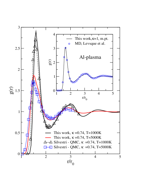
Figure 3: Ion-ion pair-distribution functions of Al from this work compared with those obtained by Silvestrisilv1 . The inset shows the comparison at normal density and at the melting point. Here no data from ref.silv1 is availble, but we use accurate molecular-dynamics simulations (Levesque et allwr ) for comparison.

A simulation box of 125 atoms implies only 5 atoms per dimension and hence even the central atom feels only two atomic shells around it. The calculation of the $\omega\to 0$ limit needed to obtain a static conductivity is also quite difficult, and one approach is to assume the validity of the Drude form and fit a free-electron Drude form to achieve this. The Kubo-Greenwod type MD procedure would nevertheless provide useful complementary results for comparison with our two-component DFT approaches, and would be of much interest in studying low-temperature systems with a tendency to covalent bonding and clustering. However, these methods bring in a number of approximations of their own and need cautious reconsideration. In this context, an interesting test would be to examine expanded liquid-Hgbhat using the Kubo-Greenwood MD approach.

Figure 4: Dynamic conductivity (au.) of Al at a compression of 0.25 at $T$ =2.5 eV and 10 eV. The Drude conductivity is modified by the presence of the $3s$ level. Time-dependent DFT calculation greatly weakens the effect.

III.3 Dynamic conductivity from time-dependent density functional theory.

Time dependent DFT provides a convenient approach to the calculation of the dynamic conductivity of interacting systems. The TDFT formulation relevant to dense plasmasgri includes dynamic screening and coupling to ion-dynamics in a computationally convenient, self-consistent manner. The main consequence of the TDFT formulation is to replace, say, the dipole matix elements $<i|\vec{r}|j>$ between states $i,j$ by a dynamic form $<i|\vec{r}(\omega)|j>$ where the modification of the driving field by the response of the system is taken into account in a self-consistent manner. Consider a weak external field $\vec{E}_{ext}(t)$ = $\vec{E}cos(\omega t)$. This corresponds to an external potential:

$$U_{ext}(\vec{r},t)=e\vec{r}\cdot E_{ext}(t)$$ (29)

The dipole form of the interaction is used since one of the objectives is to include the corrections arising from the presence of bound states. However, the dipole form of the matrix elements can be easily replaced by the momentum or acceleration formulation when needed. We assume that the electric field is directed along the z-direction, and suppress vector notation for the field unless needed. The external potential induces an electron density fluctuation $\delta n(r)$ which in turn generates corrections to the Coulomb and exchange-correlation potentials. Since the linear absorption coefficient (or optical conductivity) is the object of our study, $\delta n(r)$ etc., can be written in terms of the electron response function $\chi^{0}(r,r^{\prime}|\omega)$ which can be approxmiately constructedgri from the Kohn-Sham eigenstates of the plasma. Then we have

$$U(\vec{r},\omega) = U_{ext}(\vec{r},\omega)+V^{c}_{ind}+V^{xc}_{ind}$$ (30)

$$V^{c}_{ind} = \int d\vec{r^{\prime}}\frac{\delta n(\vec{r},\omega)}{|\vec{r}-\vec{r^{\prime}}|}$$ (31)

$$V^{xc}_{ind} = \left[\frac{\partial V_{xc}(\vec{r},\omega)}{\partial n(\vec{r},\omega)}\right]\delta n(\vec{r},\omega)$$ (32)

$$\delta n(\vec{r},\omega) = \int d\vec{r^{\prime}}\chi(\vec{r},\vec{r^{\prime}}|\omega)U(\vec{r^{\prime}},\omega)$$ (33)

Here $V^{xc}_{ind}(r)$ is calculated from the gradient $\partial V_{xc}/\partial n$ evaluated at the density $n_{0}(r)$ in the unperturbed neutral pseudo atom. Since the form of the time-dependent exchange-correlation potential $V_{xc}(r,\omega)$ is still not established, most implementations use the static $V_{xc}[n(r)]$ of ordinary density functional theory. The above set of equations have to be solved self consistently to obtain the total perturbing potential $U(\vec{r},\omega)$. In effect, the dipole operator, or equivalently, the momentum operator of the scattering electron is replaced by a space and time dependent quantity which enters into the polarizability. Given the spherical symmetry of the system, the total perturbing potential has the form

$$U(\vec{r},\omega)=-(1/2)EU_{\omega}(r)Y^{0}_{1}(\vec{r}/r)$$ (34)

Here $Y^{0}_{1}$ is a spherical harmonic. If we ignored these induced fields, the conductivity of the system can be written as:

$$\Re\,\sigma^{0}(\omega)=\frac{e^{2}}{a_{0}\hbar}\Im\,\sum_{\nu,\nu^{\prime}}\frac{\pi N_{i}\omega}{3}\frac{|<\nu|r|\nu^{\prime}>|^{2}(f_{\nu}-f_{nu^{\prime}})}{\omega+\epsilon_{\nu}-\epsilon_{\nu}^{\prime}+i\delta}$$ (35)

Here all the quantities on the right of the summation are in atomic units. The $e^{2}/(a_{0}\hbar)$ factor is the atomic unit of conductivity. $N_{i}$ is the number of ions per unit volume, and we neglect the effect of ion-ion correlations in the bound-free and bound-bound processes. (It can be shown that these contribute mainly to the width of the transition by broadening the levels) Also when $\nu,\nu^{\prime}$ = $k,l,m$ and $k^{\prime},l^{\prime}m^{\prime}$ for free-free transitions, the dipole matrix element is replaced by the momentum form, i.e, $|<\nu|\vec{r}|\nu^{\prime}>|^{2}$ = $|<\nu|\vec{\nabla}|\nu^{\prime}>|^{2}/\omega^{2}$.

The conductivity expression $\sigma^{0}(\omega)$ is known to be particularly inadequate when treating b-f and b-b processes, unless the initial bound state is a deep lying (e.g, 1s) statekedge . Hence we need to include the induced fields in treating under-dense plasmas where there is a bound state close to ionization. This involves the use of the total perturbing potential, $U(\vec{r},\omega)$, rather than the external potential $\vec{r}\cdot\vec{E}$ in constructing the matrix elements contained in the conductivity expression:

$$\Re\,\sigma(\omega)=\frac{N_{i}\pi\omega}{3}\Im\sum_{\nu,\nu^{\prime}}$$

$$|<\nu|U_{\omega}(r)Y^{0}_{1}(\vec{r}/r)|\nu^{\prime}>|^{2}*(f_{\nu}-f_{nu^{\prime}})\delta(\omega+\epsilon_{\nu}-k^{2}/2)$$

The effect of level broadening can be included in the above expression by replacing the delta function $\delta(\omega+\epsilon_{\nu}-k^{2}/2)$ by a form containing the self-energy corrections to the single-particle levels, as in Grimaldi et al, where self-energies were calculated. However, for our present purpose, we use the $\tau$ used in the Drude calculation to provide a broadening parameter. In fact, we have shown in Ref. dyson-mott that the self-energy contribution of ion-electron scattering to level broadening is identical to that given by the Ziman formula. Thus, setting $\gamma=1/\tau$, we replace the $\delta$-function in the above equation with a Lorentzian.

$$\delta(\omega+\epsilon_{\nu}-k^{2}/2)\to\frac{\gamma/\pi}{(\omega+\epsilon_{\nu}-k^{2}/2)^{2}+\gamma^{2}}$$

III.4 Some numerical results.

In this section we present results for the dynamic conductivity of some Al-plasmas to illustrate the effect of the scattering events where shallow bound states modify the Drude-like conductivity. These “bound states” are really Kohn-Sham eigenvalues and hence their values may need improvement by evaluating the corrections using a Dyson equation.dyson-mott The first step of the calculation is the solution of the NPA model to obtain the Kohn-Sham basis set $\{\phi(r)_{\nu}\}$ for the given electron density and temperature. The codes necessary for the NPA calculation, the resistivity calculation, as well as the plasma conditions (EOS) that go into the resistivity or conductivity calculations may be accessed via the internet at our websiteweb .

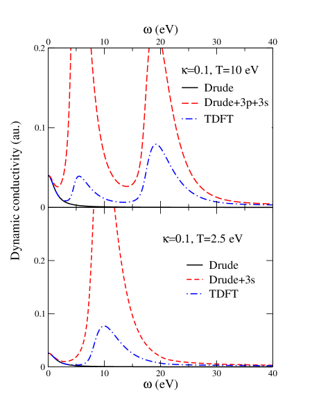
Figure 5: Dynamic conductivity (au.) of Al at a compression of 0.1 at $T$ =2.5 eV and 10 eV. The Drude conductivity is modified by the presence of shallow $3s$ at $T$ = 2.5 eV, and also the $3p$ level at 10 eV. The effect is reduced in the TDFT calculation.

Some results for the shallow bound states present in $Al$-plasmas at T=2.5 eV and 10 eV, for compressions $\kappa=0.25$, and 0.1 are given in table II. In the T=10, $\kappa=0.1$ case we have two shallow bound states, viz., $3s$ and $3p$. In Table 3 their occupation numbers and the interacting chemical potential needed for calculating the Fermi factors are given. In calculating the matrix element $|<nlm|r|kl^{\prime}m^{\prime}>|^{2}$, the correct density of states $\aleph(\epsilon)$ for the continuum state $|kl^{\prime}m^{\prime}>$, normalized in a sphere of radius $R$, with $R\to\infty$ should be included. That is,

$$k_{n}R-\pi l/2 = n\pi+\delta_{kl}$$

$$\aleph(\epsilon) = \frac{\partial n}{\partial k}\frac{\partial k}{\partial\epsilon}$$

The calculations are very simple if (a) we ignore the Zangwill-Soven type TDFT effects arising from the reaction of the system which act to modify the external field. (b) if we ignore the phase shifts $\delta_{kl}$, and replace the boundstates by hydrogen-like states with the correct $Z=\bar{Z}$. The final results depend on the level broadening parameter $\gamma$ used in the calculation.

In fig.4 and Fig.5 we show the conductivity arising from the presence of the $3s$ and $3p$ levels, as well as the Drude term, and the modification when TDFT is included in an approximate manner. These TDFT calculations should be regarded as highly provisional results only; in fact, the treatment of shallow boundstates using DFT is itself questionable since the Kohn-Sham eigenvalues are known to be a poor approximation to the actual excitation spectrum.

III.4.1 bound-bound processes.

Clearly, the presence of a partially occupied $3s$ and a $3p$ state with an energy separation of the order of 0.46 au. would lead to a contribution from b-b processes at around 12 eV. This contribution is easily included in the calculation under the simplifying assumptions that we noted before. However, this is a relatively sharp “line” resonance which is expected to undergoes significant modification when the time-dependent effects are taken in to account. We have not included it in our figures.

Table 3: details regarding the n=3 shallow states in underdense $Al$ at T=10 eV and 2.5 eV. Full occupation is when Occ is unity

$\kappa$	0.25	0.25	0.1	0.1
$T$	2.5 eV	10 eV	2.5 eV	10 eV
$\mu$	0.0393	-0.5538	-0.6652	-0.9589
Occ(3s)	0.7444	,0.2217	0.6850	0.1455
Occ(3p)	–	–	–	0.0843

IV Conclusion.

The first-principles calculation of the dynamic conductivity of warm dense matter may be conveniently carried out within the framework of multi-component density functional theory. The static calculation (NPA etc) provides the Kohn-Sham basis set, phase shifts, pseudopotentials for constructing ion-ion pair potentials and structure factors. These immediately provide results for the static conductivity. Further, the energy-levels and occupation numbers obtained from the Kohn-Sham NPA solution can be the starting approximation for a time-dependent density functional calculation of the optical conductivity. This proceeds in much the same way as the optical absorption cross section. Details of such a time-dependent calculation, based on the method of Zangwill and Soven, may be found in Grimaldi, Lecourte and Dharma-wardana.gri

References

- (1) F. Perrot and M.W.C. Dharma-wardana, Phys. Rev. A 36,238 (1987)
- (2) F. Perrot and M.W.C. Dharma-wardana,Phys. Rev. E. 52, 2920 (1995); Int. J. Thermophys. 20, 1299 (1999)
- (3) J. F. Benage, W. R. Shanahan and M. S. Murillo, Phys. Rev. Lett. 83, 2953 (1999)
- (4) C. Niemann, L. Divol, D. H. Froula, G. Gregori, O. Jones, R. K. Kirkwood, A. J. McKinnon, N. B. Meezan, J. D. Moody, C. Sorce, L. J. Suter, R. Bahr, W. Seka, and S. H. Glenzer, Phys. Rev. Lett., 94, 85005 (2005)
- (5) A. Forsman, A. Ng, G. Chiu, and R. M. More, Phys. Rev. E 58, R1248-R1251 (1998)
- (6) A. Ng, T. Ao, F. Perrot, M. W. C. Dharma-wardana and M. E. Foord, http://arxiv.org/physics-0505070 ; to appear in Lasers and Particle Beams.
- (7) D. M. Ceperley, Recent Progress in Many-body Theories, Ed. J. B. Zabolitsky (springer, Berlin 1981), p262
- (8) I. Kwon, L. Collins, J. Kress and N. Troullier, Phys. Rev. E. 54, 2844 (1996)
- (9) Y. T. Lee and R. M. More, Phys. Fluids, 27, 1273 (1984)
- (10) F. Grimaldi, A. Grimaldi-Lecourte, and M.W.C. Dharma-wardana, Phys. Rev. A 32, 1063 (1985)
- (11) F. Perrot, M.W.C. Dharma-wardana, and John Benage, Phys. Rev. E 65, 046414 (2002)
- (12) M. W. C. Dharma-wardana and François Perrot, Phys. Rev.B (2002)
- (13) R. N. Bhatt and T. M. rice, Phys. Rev. B, 20, 466 (1979)
- (14) H. Yoneda, H. Morikami, K.-i Ueda, and R. M.More, Phys. Rev. Lett., 91, 75004 (2003)
- (15) Andrew Ng, private communication.
- (16) L. J. Dagens, Phys. (Paris) 34, 879 (1973)
- (17) VASP, www.b-initio Simulation Package, AB-INIT, www GAUSSIAN, www
- (18) http://babylon.phy.nrc.ca/ims/qp/chandre/
- (19) Density Functional Theory, Ed. E. K. U. Gross and Dreizler
- (20) F. Perrot and M. W. C. Dharma-wardana, Phys. Rev. A 29, 1378 (1984)
- (21) Michael Surh, T. W. Barbee III, and L. H. Yang, Phys. Rev. Lett. 86, 5958 (2001)
- (22) R. Evans, B. L. Gyorffy, N. Szabo and J. M. Ziman, in Properties of liquid metals, Ed. S. Takeuchi (Wiley, New York, 1973)
- (23) W. W. Schulz and P. B. Allen, Phys. Rev. B 52, 7994 (1995)
- (24) C.Majumdar and W. Kohn, Phys. Rev. 138, A1617 (1965)
- (25) M.W.C. Dharma-wardana and F. Perrot, Phys. Let., A 163, 223 (1992); M.W.C. Dharma-wardana in Laser Interactions with Atoms, Solids, and Plasmas, Edited by R.M. More (Plenum, New York, 1994), p311
- (26) S. Ethier and J.-P. Matte, Phys. Plasmas 8, 1650 (2001), and references there-in.
- (27) M. Bŭttiker, A. Prètre, and H. Thomas, Phys. Rev. Lett. 70, 4114 (1993) and references there-in.
- (28) N. W. Ashcroft and K. Sturm, Phys. Rev. B, 3 1898 (1971); G Dresselhaus, M. S. Dresselhaus, and D. Beaglehole, as reported in Ashcroft and Sturm.
- (29) J. C. Miller, Phil. Mag. 20, 1115 (1969)
- (30) T. E. Faber, An introduction to the theory of liquid metals, (Cambridge University press, Cambridge,1972).
- (31) L. Benedict, C. D. Spataru, and S. G. Louie, Phys. Rev. B 66, 085116 (2002)
- (32) J. J. Hopfield, Phy. Rev. A 139, 419 (1965)
- (33) G. D. Mahan, J. Phys. Chem. Solids 31, 1477 (1970) gives a calculation for phonon scattering.
- (34) G. Röpke, R. Redmer, A. Wierling and H. Reinholz, Phys. Rev E 60 R2484 (1999)
- (35) M.W.C. Dharma-wardana and F. Perrot, Phys. Rev. E 58, 3705 (1998) and Erratum, 63, 069901 (2001)
- (36) F. Perrot and M.W.C. Dharma-wardana, Phys. Rev. B15 62, 14766 (2000)
- (37) P. L. Silvestrelli, Phys. Reb B 60, 16382 (1999); P. L. Silvestrelli, A. Alavi, and M. Parrinello, Phys. Rev. B 55, 15515 (1997)
- (38) A. Alavi, M. Parrinello, and D. Fenkel, Science, 269, 1252 (1995)
- (39) D. Levesque, J. J. Weis, and J. Reatto, Phys. Rev. Lett. 54, 451 (1985); M. W. C. Dharma-wardana and G. C. Aers, Ibid, 56, 1211 (1986)
- (40) Gillan et al, see the phonon website
- (41) A. Zangwill and P. Soven, Phys. Rev. A 21,1561 (1980)
- (42) F. Perrot and M.W.C. Dharma-wardana, Phys. Rev. Lett. 71 , 797 (1993)