Transport equation for 2D electron liquid under microwave radiation plus magnetic field and the Zero Resistance State

Abstract

A general transport equation for the center of mass motion is constructed to study transports of electronic system under uniform magnetic field and microwave radiation. The equation is applied to study 2D electron system in the limit of weak disorder where negative resistance instability is observed when the radiation field is strong enough. A solution of the transport equation with spontaneous AC current is proposed to explain the experimentally observed Radiation-Induced Zero Resistance State.

The discovery of the zero-resistance states (ZRS) in two dimensional electron gas under uniform magnetic fieldmani ; zudov and microwave radiation has triggered a lots of theoreticalt1 ; t2 ; t3 ; t4 ; t5 ; t6 ; t7 and experimental activitiese1 ; e2 to understand the origin of this nontrivial state. Most of the theoretical work suggested that the origin of the ZRS is closely related to a negative-resistance instability that occurs in the system due to the combined effect of quantized Landau levels and photon-assisted scatteringt1 ; t2 ; t3 ; t4 ; t7 . It was proposed that the ZRS can be explained if the current-dependent resistance of the system which becomes negative at small current (for strong enough microwave radiation) becomes positive again when the current $\vec{j}$ becomes large enought1 ; t2 ; t3 ; t4 . The above physics was put together phenomenologically into an equation

$$\vec{E}_{d}=\rho_{H}[\vec{j}\times\hat{z}]+R[|\vec{j}|]\vec{j}$$ (1)

where $R[j]$ is a phenomenological current-dependent resistance which is negative at $j=0$, increases as a function of $j$ and passes through zero at $|\vec{j}|=j_{o}$t4 , $\vec{E}_{d}$ is the applied DC electric field and $\rho_{H}$ is the ordinary Hall resistivity. It was shown that equation  (1) admits time-independent, stripe-like spatially inhomogeneous solution which leads to zero differential resistance for net DC current less than a threshold valuet4 . An obvious theoretical question is whether Eq. (1) with the required property of $R[j]$ can be derived microscopically. This is the subject of this paper.

Starting from first principle we shall derive in the following a transport equation for the center of mass velocity $\vec{v}=\vec{j}/ne$ that treats the effect of radiation to all order with the only expansion parameter in the problem being the strength of disorder. We note that a transport equation can also be derived from a Quantum Boltzmann Equation approacht7 . However it is difficult to obtain clear, analytical result in this approach because of the intrinsic complexity of the Boltzmann equation formulation itself. We shall see that the equation of motion for the center of mass offers a much simpler alternative.

Our approach to the transport equation begins from the known observation that there exists an exact, one-to-one mapping between the solution of the Schr$\ddot{o}$dinger equation of a (charged) many-particle system in the absence of the microwave radiation and in the presence of the radiation for a class of Hamiltoniant2 ; t5 ; t6 ; t7 ; t8 ,

$$H(t)=H_{o}-e\sum_{i}\vec{r}_{i}.\vec{E}(t)$$ (2)

where

$$H_{o}(\vec{r}_{i})=\sum_{i}{1\over 2m}(\vec{p}_{i}-{e\over c}\vec{A}(\vec{r}_{i}))^{2}+{1\over 2}\sum_{i\neq j}V(\vec{r}_{i}-\vec{r}_{j})+{1\over 2}\sum_{i}\vec{r}_{i}.\tensor{K}.\vec{r}_{i}$$ (3)

where $\vec{p}_{i}=-i\bar{h}\nabla_{i}$ is the canonical momentum for the $i^{th}$ particle in the system. $\vec{A}(\vec{r})=-{1\over 2}(\vec{r}\times\vec{B})$ is the vector potential corresponding to a uniform, time-dependent magnetic field, $\vec{E}(t)$ is a time-dependent uniform electric field and $V(\vec{r})$ is the interaction potential between particles. The last term represents an external harmonic potential acting on the particles.

The physics of the exact mapping can be seen by performing a coordinate transformation to the center of mass frame of the many-particle system. In the non-relativistic limit, the wavefunctions in the laboratory and CM frames are related by

$$\psi_{lab}(\vec{r}_{i};t)=\psi_{CM}(\vec{r}_{i}-\vec{R}(t);t)e^{i\theta(\vec{R}(t))},$$

where $\vec{R}(t)={1\over N}\sum_{i}<\vec{r}_{i}(t)>$ is the center of mass coordinate in the laboratory frame, $N=$ number of particles and $\theta(\vec{R}(t))$ is an overall phase that depends on $\vec{R}(t)$ only. The corresponding Hamiltonian in the CM frame is

$$H^{\prime}(t) = \sum_{i}{1\over 2m}(\vec{p}_{i}^{\prime}-m\dot{\vec{R}}(t)-{e\over c}\vec{A}_{CM}^{\prime}(\vec{r}_{i}^{\prime}))^{2}+{1\over 2}\sum_{i\neq j}V(\vec{r}_{i}^{\prime}-\vec{r}_{j}^{\prime})$$

$$+{1\over 2}\sum_{i}(\vec{r}_{i}^{\prime}+\vec{R}(t)).\tensor{K}.(\vec{r}_{i}^{\prime}+\vec{R}(t))-e\sum_{i}\vec{r}_{i}^{\prime}.\vec{E}^{\prime}(t)$$

where $\vec{r}^{\prime}=\vec{r}-\vec{R}(t)$, $\vec{p}_{i}^{\prime}=-i\bar{h}\nabla^{\prime}$ and $\vec{A}^{\prime}(\vec{r}^{\prime})=-{1\over 2}\vec{r}^{\prime}\times\vec{B}^{\prime}$. $\vec{B}^{\prime}=\vec{B}$ and $\vec{E}^{\prime}(t)=\vec{E}(t)+{1\over c}\dot{\vec{R}}(t)\times\vec{B}$ are the Galilean transformed magnetic and electric fields in the CM frame valid in the non-relativistic limit. The Schr$\ddot{o}$dinger equation in the CM frame, $i\hbar\dot{\psi}_{CM}=H^{\prime}(t)\psi_{CM}$ can be simplified by a performing a gauge transformation $\psi_{CM}=\phi_{CM}e^{i\Lambda(t)}$, where $\hbar\Lambda(t)=\sum_{i}\left(m\dot{\vec{R}}(t).\vec{r}^{\prime}-{1\over 2}\int^{t}dt^{\prime}\vec{R}(t^{\prime}).\tensor{K}\vec{R}(t^{\prime})\right)$. With Eq. (Transport equation for 2D electron liquid under microwave radiation plus magnetic field and the Zero Resistance State), we obtain

$$i\hbar{\partial\over\partial t}\phi_{CM}(\vec{r}^{\prime};t)=\left(H_{o}(\vec{r}^{\prime}_{i})-\sum_{i}\vec{r}^{\prime}_{i}.\vec{a}(t)\right)\phi_{CM}(\vec{r}^{\prime};t),$$ (5)

where $\vec{a}(t)=e\left(\vec{E}(t)+{1\over c}(\dot{\vec{R}}(t)\times\vec{B})\right)-\tensor{K}.\vec{R}(t)-m\ddot{\vec{R}}(t)=0$. $\vec{a}(t)$ vanishes because it is the equation of motion for $\vec{R}(t)$ derived directly from the corresponding Heisenberg equation of motion. We thus arrive at the conclusion that for the class of Hamiltonian  (2), there exist a one-to-one mapping between the solution of the Schr$\ddot{o}$dinger equation in the presence of the microwave radiation $\psi(\vec{r}_{i};t)$, and in the absence of the radiation $\phi_{CM}(\vec{r}_{i}^{\prime};t)$, where $\psi(\vec{r}_{i};t)=\phi_{CM}(\vec{r}_{i}-\vec{R}(t);t)e^{i\Lambda(t)}$. Physically, for the particular form of Hamiltonian we considered, the wavefunction of the system follows the center of mass motion rigidity in the presence of the radiation field.

The above result suggests that for more general Hamiltonians of form $H_{G}(t)=H(t)+U$, a new perturbation scheme where the microwave radiation is treated exactly to all order can be set up by treating $U$ as perturbation. The perturbation scheme can be set up most easily in the center of mass frame. We shall consider static impurity potential $U=\lambda\sum_{i}u(\vec{r}_{i})$ in the following. Notice that a static potential become time-dependent in the CM frame and should be treated by time-dependent perturbation theory.

To derive the transport equation we start from the exact Heisenberg equation of motion for the center of mass coordinate, $i\hbar\dot{\vec{R}}(t)=[\vec{R}(t),H_{G}(t)]$ with $\tensor{K}=0$t2 . We obtain after some simple algebra

$$m\ddot{\vec{R}}(t)=e\left(\vec{E}(t)+{1\over c}(\dot{\vec{R}}(t)\times\vec{B})\right)-{\lambda\over N}\int d^{d}r\left(\nabla u(\vec{r})\right)n(\vec{r},t)$$ (6)

where $n(\vec{r},t)=\sum_{i}<\delta(\vec{r}-\vec{r}_{i})>$ is the time-dependent average electron density. In the CM frame where $n(\vec{r},t)=n_{CM}(\vec{r}-\vec{R}(t),t)$, we obtain for small $\lambda$ from linear-response theory

$$n_{CM}(\vec{r}^{\prime},t)=n^{(0)}_{CM}(\vec{r}^{\prime})+\lambda\int d^{d}r"dt"\chi(\vec{r}^{\prime}-\vec{r}";t-t^{\prime})u(\vec{r}"+\vec{R}(t^{\prime})),$$

where $\chi(\vec{r}^{\prime}-\vec{r}";t-t^{\prime})$ is the (equilibrium) retarded density-density response function in CM frame derived with the Hamiltonian $H_{o}$. Going back to the laboratory frame and performing the disorder-average $<u(\vec{r}>=0$ and $<u(\vec{r})u(\vec{r}^{\prime})>=|u|^{2}\delta(\vec{r}-\vec{r}^{\prime})$, we obtain to second order in $\lambda$, an impurity-averaged equation of motion for $\vec{R}(t)$ in laboratory framet2 ,

$$m\ddot{\vec{R}}(t)=e\left(\vec{E}(t)+{1\over c}(\dot{\vec{R}}(t)\times\vec{B})\right)+\alpha\nabla_{\vec{R}(t)}\int dt^{\prime}\chi(\vec{R}(t)-\vec{R}(t^{\prime});t-t^{\prime})$$ (7)

where $\bar{n}=N/V$ and $\alpha=\lambda^{2}|u|^{2}/\bar{n}$. The equation is manifestly gauge invariant and suggests that to second order in the impurity potential, the effects of particle statistics and interaction are reflected only in the density-density response function. In the following we shall apply this equation to study the ZRS in 2D electron systems.

In this case we consider $\vec{E}(t)=\vec{E}_{o}\sin(\omega t)+\vec{E}_{d}$, where $\vec{E}_{d}$ is a small DC electric field. To simplify the equation we divide the center of mass motion into ”fast” and ”slow” parts,

$$\vec{R}(t)=\vec{R}_{f}(t)+\vec{R}_{s}(t)\sim\vec{A}_{o}\cos(\omega t)+\vec{B}_{o}\sin(\omega t)+\vec{R}_{s}(t).$$ (8)

$\vec{R}_{f}(t)$ describes the center of mass motion induced by the radiation field whereas $\vec{R}_{s}(T)$ describes induced motion under the DC field $\vec{E}_{d}$. The two kinds of motions are coupled by the impurity scattering term which is a non-linear function of $\vec{R}(t)$. We shall assume that the coupling between $\vec{R}_{s}(t)$ and $\vec{R}_{f}(t)$ does not modify qualitatively the behavior of $\vec{R}_{f}(t)$ and the main effect of coupling is to produce an effective equation of motion for $\vec{R}_{s}(t)$. Notice that we keep only the first harmonic terms in $\vec{R}_{f}(t)$ in Eq. (8). This is valid in the small $\vec{E}_{o}$ limit when the size of the orbit $R_{c}\sim\sqrt{\vec{A}_{o}^{2}+\vec{B}_{o}^{2}}$ is much less than the magnetic length $l=(\hbar c/eB)^{1/2}$ and is justifiable under the experimental conditionmani ; zudov where the magnetic field is weak and the magnetic length is very long.

To treat the impurity scattering term we write $\nabla_{\vec{R}(t)}\int_{-\infty}^{t}dt^{\prime}\chi(\vec{R}(t)-\vec{R}(t^{\prime});t-t^{\prime})=-\int\vec{q}d^{d}q\int{d\omega^{\prime}\over\pi}Im\chi(\vec{q},\omega^{\prime})\int_{-\infty}^{t}dt^{\prime}e^{i[\vec{q}.(\vec{R}(t)-\vec{R}(t^{\prime}))-\omega^{\prime}(t-t^{\prime})]}$, where $\chi(\vec{q},\omega)$ is the Fourier transform of $\chi(\vec{r};t)$. To evaluate the integral over $t^{\prime}$ we make the local approximation $\vec{R}_{s}(t)-\vec{R}_{s}(t^{\prime})\sim\vec{v}(t)(t-t^{\prime})+{1\over 2}\dot{\vec{v}}(t)(t-t^{\prime})^{2}$, and

$$\int_{-\infty}^{t}dt^{\prime}e^{i[\vec{q}.(\vec{R}(t)-\vec{R}(t^{\prime}))-\omega^{\prime}(t-t^{\prime})]}\sim\int_{-\infty}^{t}dt^{\prime}e^{i[\vec{q}.(\vec{R}_{f}(t)-\vec{R}_{f}(t^{\prime}))+\left(\vec{q}.\vec{v}(t)-\omega^{\prime}\right)(t-t^{\prime})]}\left(1+i\vec{q}.\dot{\vec{v}}(t){(t-t^{\prime})^{2}\over 2}\right)$$

valid for $\vec{v}(t+T^{\prime})-\vec{v}(t)<<\vec{v}(t)$, where $T^{\prime}\sim 2\pi/\omega_{B}$ is the characteristic time-scale for the density response. The $\vec{R}_{f}(t)-\vec{R}_{f}(t^{\prime})$ term can be expanded in a series of $\vec{A}_{o},\vec{B}_{o}$ using the identity $e^{ix\sin\theta}=\sum_{m}J_{m}(x)e^{im\theta}$. We obtain after some algebra,

$$\nabla_{\vec{R}(t)}\int_{-\infty}^{t}dt^{\prime}\chi(\vec{R}(t)-\vec{R}(t^{\prime});t-t^{\prime}) = \sum_{m,m^{\prime}}e^{i(m-m^{\prime})(\omega t+\theta)}\int\vec{q}d^{d}qJ_{m}(z(\vec{q}))J_{m^{\prime}}(z(\vec{q}))$$

$$\times\left(1-i{\vec{q}.\dot{\vec{v}}(t)\over 2}{\partial^{2}\over\partial\omega^{\prime 2}}\right)\chi(\vec{q},\omega^{\prime})_{\omega^{\prime}=m\omega+\vec{q}.\vec{v}(t)}$$

where $z(\vec{q})=\sqrt{(\vec{q}.\vec{A}_{o})^{2}+(\vec{q}.\vec{B}_{o})^{2}}$ and $\tan\theta=\vec{q}.\vec{A}_{o}/\vec{q}.\vec{B}_{o}$t2 . We shall consider $z(\vec{q})^{2}=R_{c}^{2}q^{2}/2$ in the following corresponding to circularly polarized lightt7 . In this case the response of the system is isotropic and the computation is much simplified. The effective force on $\vec{R}_{s}(t)$ is derived from the $m=m^{\prime}$ terms in  (Transport equation for 2D electron liquid under microwave radiation plus magnetic field and the Zero Resistance State). To order $(R_{c}/l)^{2}$ we keep only $m(m^{\prime})=0,1$ terms. Putting it back into the equation of motion  (7), we obtain

$$\left(m+\Pi[\omega,|\vec{v}(t)|]\right)\dot{\vec{v}}(t)=e\vec{E}_{d}+{e\over c}(\vec{v}(t)\times\vec{B})-R[\omega,|\vec{v}(t)|]\vec{v}(t),$$ (10)

where $\omega$ is the frequency of the microwave radiation, and

$$R[\omega,\vec{v}] \sim {\alpha\over v^{2}}\int\vec{q}.\vec{v}d^{d}q\left[(1-{z(\vec{q})^{2}\over 2})Im\chi(\vec{q},\vec{q}.\vec{v})+{z(\vec{q})^{2}\over 4}Im\chi(\vec{q},\omega+\vec{q}.\vec{v})\right],$$ (11)

$$\Pi[\omega,\vec{v}] \sim -{\alpha\over 4}\int q^{2}d^{d}q{\partial^{2}\over\partial\omega^{\prime 2}}\left[(1-{z(\vec{q})^{2}\over 2})Re\chi(\vec{q},\omega^{\prime})_{\omega^{\prime}=\vec{q}.\vec{v}}+{z(\vec{q})^{2}\over 4}Re\chi(\vec{q},\omega^{\prime})_{\omega^{\prime}=\omega+\vec{q}.\vec{v}}\right].$$

It is obvious that $R[\omega,\vec{v}]$ represents dissipative response of the electron gas to external perturbations whereas $\Pi[\omega,\vec{v}]$ is an effective mass correction on the center of mass motion coming from the corresponding reactive response. Negative contributions to the resistance shows up in the second term of $R$ for density-density response functions with resonant structure, $\chi(\vec{q},\omega)\sim\sum_{n}{g_{n}(\vec{q})\over\pi}{-2\omega_{n}\over\omega^{2}-\omega_{n}^{2}}$, where $\omega_{n}>0$ are resonant energy levels and $g_{n}(\vec{q})$ is a positive definite function. In this case, $R\sim\sum_{n}\left(R_{1n}\omega_{n}+R_{2n}(\omega_{n}-\omega)\right)$, where $R_{1n}$ and $R_{2n}$ are positive definite numbers. We see that negative contributions to $R_{2}$ exist for $\omega_{n}<\omega$. The physical origin of the negative resistance has been discussed in several earlier workst1 ; t2 ; t3 ; t4 ; t7 and we shall not repeat them here. Correspondingly, the effective mass contribution from level $n$ is positive (negative) when $\omega>(<)\omega_{n}$. We note that the effective mass correction originates from the impurity scattering term is of order $\Pi[\omega,v]\sim m\times(1/\omega_{B}\tau)<<m$ in the weak-disorder limit, where $\omega_{B}=eM/mc$ is the cyclotron frequency and $\tau\sim(g_{2d}\lambda^{2}|u|^{2})^{-1}$ is the elastic lifetime. Eq. (10) differs from the phenomenological equation  (1) mainly in the presence of the inertial term $m\dot{\vec{v}}$ which allows the system to admit time-dependent solutions in the present case.

To see whether $R[\omega,v]$ has the expected behavior we consider density response function of non-interacting gases wheret2 $\chi(\vec{q},\omega)=(2\pi l^{2})^{-1}\sum_{m,n}(n_{2}!/n_{1}!)\left(Q^{2}/2\right)^{n_{1}-n_{2}}e^{-(Q^{2}/2)}\left(L^{n_{1}-n_{2}}_{n_{2}}(Q^{2}/2)\right)^{2}\left({n_{F}(n\omega_{B})-n_{F}(m\omega_{B})\over\omega+(n-m)\omega_{B}+i\delta}\right)$, where $n_{1}=\max(n,m)$, $n_{2}=\min(n,m)$, $L^{n}_{m}(x)$ is the associated Laguerre polynomials, $n_{F}(\epsilon)$ is the Fermi distribution function and $Q^{2}=|\vec{q}|^{2}l^{2}$. To incorporate inelastic lifetime effects we also introduce a phenomenological broadening $\Gamma(T)$ to the Landau levels, i.e. $\delta(\epsilon-n\omega_{B})\rightarrow(\pi)^{-1}\Gamma/((\epsilon-n\omega_{B})^{2}+\Gamma^{2})$. $R[\omega,\vec{v}]$ is evaluated numerically with these approximations. In figure one we present numerical results for the normalized resistance $R(\omega,v)/R(0,0)$, as a function of normalized velocity $v_{N}=v/(l\omega_{B})$ for $\omega/\omega_{B}=0,0.85,1.0,1.1,1.2$, taking $(R_{c}/l)^{2}=0.1$, $E_{F}\sim 10\omega_{B}$, $T=2\omega_{B}$, $\Gamma=0.5$ and keeping $20$ levels in the sum. We observe that $R(\omega,v\rightarrow 0)$ becomes negative when $\omega\gtrsim\omega_{B}$, in agreement with previous resultst7 . For $\omega>\omega_{B}$ $R(\omega,v)$’s increases and cross zero at around $v_{oN}\sim 0.05$. The effect of microwave radiation decreases rapidly for $v_{N}\gtrsim 0.2$. These qualitative behaviors of $R(\omega,v)$ are in agreement with expectation and are not modified by changing $T$ or $\Gamma$.

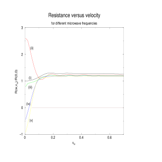
Figure 1: Normalized resistance as a function of velocity for $\omega/\omega_{B}=0(i),0.85(ii),1.0(iii),1.1(iv),1.2(v)$.

Eq. (10) allows time-dependent solutions. In the absence of the DC field, a simple, spatially homogeneous solution which allows the system to stabilize itself around the point $v_{o}=(l\omega_{B})v_{oN}$ is

$$\vec{v}^{(0)}(t)=R_{o}(\cos(\omega_{s}t)\hat{(}x)+\sin(\omega_{s}t)\hat{(}y)),$$

with $R_{o}=v_{o}/\omega_{s}$ where $\omega_{s}=eB/(m+\Pi(\omega,v_{o}))c\sim\omega_{B}$. The solution represents a collective circular motion of the whole fluid moving with speed $v_{o}$. Notice that a time-independent, spatially inhomogeneous solution corresponding to a pattern of alternating current stripest6 still exist. However this solution is energetically less favorable because it requires a higher energy to create the charge inhomogeneity needed to maintain the stripes of currents.

To understand the ZRS we have to consider the boundaries of the droplet of electron fluid. For sharp boundaries the boundary condition $j_{\bot}=0$ has to be imposed where $j_{\bot}$ is the component of current perpendicular to the boundary. As a result an edge region with a time-independent current $j_{//}\sim j_{o}$ must form. The size of this region is determined by the microscopic charge dynamicst4 which is still undetermined. Nevertheless according to Eq. (10) an electric field perpendicular to the boundary with magnitude $\sim E_{d}=Bv_{o}/c$ has to be present in this region to maintain the steady current flow. A similar edge region also exists at the opposite edge with a current running in the opposite direction, rather similar to edge states in Quantum Hall Effect.

A state with a small net current flow can be created with minimal disturbance to the system by shrinking the size of one edge region and enlarging the other. In this case, the net voltage drop across the sample is given by

$$V_{y}=\int E(y)dy={B\over c}\int v_{x}(y)dy={B\over ne^{2}c}\int j_{x}(y)dy=\rho_{H}I_{x},$$

corresponding to a resistance matrix with $\rho_{xx}=0$ and $\rho_{xy}=\rho_{H}$, i.e. the ZRS.

Some comments about the validity of our theory is in order. We note that in deriving Eq. (10) we made the local approximation which assumes slowly varying $\vec{v}(t)$ whereas the spontaneous current state we propose oscillate with a frequency $\sim\omega_{B}$. The oscillatory solution is allowed because of the presence of the inertia term $m\dot{\vec{v}}(t)$. Our analysis shows that the correction to the inertia term is small ($\sim m/(\omega_{B}\tau)$) in the limit of weak disorder and the local approximation mainly affects $R[\omega,v]$. Therefore our general description of the ZRS should remain valid as long as the qualitative property of $R[\omega,v]$ is correct. Another simplification we employed in our analysis is the assumption of circularly polarized light. The response of the system which is isotropic in this approximation would become anisotropic when this assumption is relaxedt2 ; t7 .

Lastly we made a comment on the macroscopic nature of the spontaneous current state we proposed. We note that in general a spontaneous current state with $|\vec{v}(t)|=v_{o}$ is characterized by a position and time dependent (2D) unit vector field $\hat{n}(\vec{x},t)$ representing the direction of the current. The order parameter field $\hat{n}(\vec{x},t)$ has the same symmetry as the ordinary 2D $x-y$ model, or superfluids. The main difference between the ZRS state and superfluids is that the rigidity of the order parameter is protected by repulsive interaction in the case of superfluids, whereas it is protected by the principle of least dissipation in the ZRS. The similarity between the two systems suggests that the two systems may share some common macroscopic features. For example, vortex-like solitonic excitations may exist in the ZRS and may lead to the residue resistance $\sim R_{o}exp(-(T_{o}/T))$ observed in the ZRS statemani ; zudov . The existence and nature of solitonic excitations depends on the detailed current dynamics of the ZRS state and will be investigated in a coming paper.

Acknowledgements This work is supported by HKRGC through Grant 602803.

References

• (1) R. Mani et.al., Nature 420, 646 (2002).
• (2) M.A. Zudov, R.R. Du, L.N. Pfeiffer and K.W. West, Phys.Β Rev.Β Lett.Β 90, 0468071(2003).
• (3) A.C. Durst, S. Sachdev, N. Read and S.M. Girvin, Phys.Β Rev.Β Lett.Β 91, 086803(2003).
• (4) X.L. Lei and S.Y. Liu, Phys.Β Rev.Β Lett.Β 91, 226805(2003).
• (5) Junren Shi and X.C. Xie, Phys.Β Rev.Β Lett.Β 91, 086801(2003).
• (6) A.V. Andreev, I.L. Aleiner and A.J. Millis, Phys.Β Rev.Β Lett.Β 91, 056803(2003).
• (7) K. Park, Phys.Β Rev.Β B69, 201301(2004).
• (8) J. I$\tilde{n}$arrea and G. Platero, Phys.Β Rev.Β Lett.Β 94, 016806(2005).
• (9) C.L. Yang et.al., Phys.Β Rev.Β Lett.Β 91, 096803(2003).
• (10) J. Zhang et.al., Phys.Β Rev.Β Lett.Β bf 92, 156802(2004).
• (11) M.G. Vavilov and I.L. Aleiner, Phys.Β Rev.Β B69, 035303(2004); I.A. Dmitriev et.al., Phys.Β Rev.Β B71, 115316(2005).
• (12) J.F. Dobson, Phys.Β Rev.Β Lett.Β 73, 2244(1994).