Generalized canonical ensembles and ensemble equivalence

Abstract

This paper is a companion article to our previous paper (J. Stat. Phys. 119, 1283 (2005), cond-mat/0408681), which introduced a generalized canonical ensemble obtained by multiplying the usual Boltzmann weight factor $e^{-\beta H}$ of the canonical ensemble with an exponential factor involving a continuous function $g$ of the Hamiltonian $H$. We provide here a simplified introduction to our previous work, focusing now on a number of physical rather than mathematical aspects of the generalized canonical ensemble. The main result discussed is that, for suitable choices of $g$, the generalized canonical ensemble reproduces, in the thermodynamic limit, all the microcanonical equilibrium properties of the many-body system represented by $H$ even if this system has a nonconcave microcanonical entropy function. This is something that in general the standard ($g=0$) canonical ensemble cannot achieve. Thus a virtue of the generalized canonical ensemble is that it can be made equivalent to the microcanonical ensemble in cases where the canonical ensemble cannot. The case of quadratic $g$-functions is discussed in detail; it leads to the so-called Gaussian ensemble.

I Introduction

The study of many-body systems having nonconcave entropy functions has been an active topic of research for some years now, with fields of study ranging from nuclear fragmentation processes D’Agostino et al. (2000); Gross (1997, 2001), and phase transitions in general Chomaz et al. (2001); Gulminelli and Chomaz (2002); Touchette and Ellis (2005), to statistical theories of stars formation Lynden-Bell and Wood (1968); Lynden-Bell (1999); Chavanis (2002); Chavanis and Ispolatov (2002); Chavanis (2003); Chavanis and Rieutord (2003), as well as statistical theories of fluid turbulence Ellis et al. (2000, 2002). The many different systems covered by these studies share an interesting particularity: they all have equilibrium properties or states that are seen in the microcanonical ensemble but not in the canonical ensemble. Such microcanonical nonequivalent states, as they are called, directly arise as a result of the nonconcavity of the entropy function, and can present themselves in many different ways both at the thermodynamic level (e.g., as negative values of the heat capacity Lynden-Bell (1999); Thirring (1970)) and the level of general macrostates (e.g., as canonically-unallowed values of the magnetization Ellis et al. (2000); Ellis and Touchette (2004)).

The fact that the canonical ensemble misses a part of the microcanonical ensemble when the entropy function of that latter ensemble is nonconcave can be understood superficially by noting two mathematical facts:

(i) The free energy function, the basic thermodynamic function of the canonical ensemble, is an always concave function of the inverse temperature.

(ii) The Legendre(-Fenchel) transform, the mathematical transform that normally connects the free energy to the entropy, and vice versa, only yields concave functions.

Taken together, these facts tell us that microcanonical entropy functions that are nonconcave cannot be expressed as the Legendre(-Fenchel) transform of the canonical free energy function, for otherwise these entropy functions would be concave. One should accordingly expect in this case to observe microcanonical equilibrium properties that have absolutely no equivalent in the canonical ensemble, since the energy and the temperature should then cease to be related in a one-to-one fashion, as is the case when the entropy function is strictly concave. This is indeed what is predicted theoretically Eyink and Spohn (1993); Ellis et al. (2000) and what is observed in many systems, including self-gravitating systems Lynden-Bell and Wood (1968); Lynden-Bell (1999); Chavanis (2002); Chavanis and Ispolatov (2002); Chavanis (2003); Chavanis and Rieutord (2003), models of fluid turbulence Ellis et al. (2000, 2002), atom clusters Schmidt et al. (2001); Gobet et al. (2002), as well as long-range interacting spin models Dauxois et al. (2000); Ispolatov and Cohen (2000); Barré et al. (2001); Dauxois et al. (2002); Antoni et al. (2002); Ellis et al. (2004); Costeniuc et al. (2004a) and models of plasmas Smith and O’Neil (1990).

What we present in this paper comes as an attempt to specifically assess the nonequivalent properties of a system which are seen at equilibrium in the microcanonical ensemble but not in the canonical ensemble. Obviously, one way to predict or calculate such properties is to proceed directly from the microcanonical ensemble. However, given the notorious intractability of microcanonical calculations , it seems sensible to consider the possibility of modifying or generalizing the canonical ensemble in the hope that it can be made equivalent with the microcanonical ensemble while preserving its analytical and computational tractability. Our aim here is to show how this idea can be put to work in two steps: first, by presenting the construction of a generalized canonical ensemble, and, second, by offering proofs of its equivalence with the microcanonical ensemble. Our generalized canonical ensemble, it turns out, not only contain the canonical ensemble as a special case, but also incorporates the so-called Gaussian ensemble proposed some years ago by Hetherington Hetherington (1987). The proofs of equivalence that we present here for the generalized canonical ensemble also apply therefore to the Gaussian ensemble.

Much of the content of the present paper has been exposed in a previous paper of ours Costeniuc et al. (2004b). The reader will find in that paper a complete and rigorous mathematical discussion of the generalized canonical ensemble. The goal of the present paper is to complement this discussion by presenting it in a less technical way than previously done and by highlighting a number physical implications of the generalized canonical ensemble which were not discussed before.

The content of the paper is as follows. In the next section, we review the theory of nonequivalent ensembles so as to set the notations and the basic results that we seek to generalize in this paper. This section is also meant to be a review of the definitions of the microcanonical and canonical ensembles. In Section III, we then present our generalization of the canonical ensemble and give proofs of its equivalence with the microcanonical ensemble for both the thermodynamic level and the macrostate level of statistical mechanics. Section V specializes these considerations to the special case of the Gaussian ensemble. We briefly comment, finally, on our ongoing work on applications of the generalized canonical ensemble.

II Review of nonequivalent ensembles

We consider, as is usual in statistical mechanics, an $n$-body system with microstate $\omega\in\Omega_{n}$ and Hamiltonian $H(\omega)$; $\Omega_{n}$ is the microstate space. Denoting the mean energy of the system by $h(\omega)=H(\omega)/n$, we define the microcanonical entropy function of the system by the usual limit

$$s(u)=\lim_{n\rightarrow\infty}\frac{1}{n}\ln\rho_{n}(u),$$ (1)

where

$$\rho_{n}(u)=\int_{\{\omega\in\Omega_{n}:h(\omega)=u\}}d\omega=\int_{\Omega_{n}}\delta(h(\omega)-u)d\omega$$ (2)

represents the density of microstates $\omega$ of the system having a mean energy $h(\omega)$ equal to $u$. As is well-known, $s(u)$ is the basic function for the microcanonical ensemble from which one calculates the thermodynamic properties of the system represented by $h(\omega)$ as a function of its energy $nu$. The analogous function for the canonical ensemble which is used to predict the thermodynamic behavior of the system as a function of its temperature $T=(k_{B}\beta)^{-1}$ is the free energy function $\varphi(\beta)$. The latter function is taken here to be defined by the limit

$$\varphi(\beta)=\lim_{n\rightarrow\infty}-\frac{1}{n}\ln Z_{n}(\beta),$$ (3)

where

$$Z_{n}(\beta)=\int_{\Omega_{n}}e^{-n\beta h(\omega)}d\omega$$ (4)

denotes, as usual, the partition function of the system at inverse temperature $\beta=(k_{B}T)^{-1}$.

Figure 1: Geometric interpretation of supporting lines in relation to the graph of the microcanonical entropy function $s(u)$ (full line) and its concave envelope or concave hull $s^{**}(u)$ (dashed line). The point $a$ in the figure has the property that $s(u)$ admits a supporting line at $a$; i.e., there exists a line passing through $(a,s(a))$ that lies above the graph of $s(u)$. In this case, $s(a)=s^{**}(a)$. The point $b$ in the figure has the property that $s(u)$ admits no supporting line at $b$. In this case $s(b)\not=s^{**}(b)$.

The entropy and free energy functions are obviously two different functions that refer to two different physical situations—the first to a closed system having a fixed energy, the second to an open system in contact with a heat bath having a fixed inverse temperature. However, these two functions are not independent. In fact, we only have to rewrite the integral defining the partition function $Z_{n}(\beta)$ as an integral over the mean energy values

$$Z_{n}(\beta)=\int\rho_{n}(u)e^{-n\beta u}du$$ (5)

rather than an integral over $\Omega_{n}$, and then approximate the resulting integral using Laplace’s method, to see that

$$Z_{n}(\beta)\approx\exp\left(-n\inf_{u}\{\beta u-s(u)\}\right)$$ (6)

with subexponential correction factors in $n$. This application of Laplace’s approximation is quite standard in statistical mechanics and leads us hitherto to the following important equation:

$$\varphi(\beta)=\inf_{u}\{\beta u-s(u)\},$$ (7)

which expresses $\varphi(\beta)$ as the Legendre-Fenchel (LF) transform of $s(u)$ Ellis (1985); Ellis et al. (2000). In convex analysis, the LF transform is often abbreviated by the notation $\varphi=s^{*}$, and $s^{*}$ in this context is called the dual of $s$ Rockafellar (1970); Ellis (1985); Ellis et al. (2000). It can be shown that the basic relationship $\varphi=s^{*}$ holds no matter what shape $s(u)$ has, be it concave or not Ellis et al. (2000). Consequently, $\varphi(\beta)$ can always be calculated from the microcanonical ensemble by first calculating $s(u)$ and then take the LF transform of this latter function. That this procedure always yield the correct free energy function $\varphi(\beta)$ follows basically from the fact that $\varphi(\beta)$ is an always concave function of $\beta$ Ellis (1985).

It is the converse process, that is, the attempt of calculating $s(u)$ from the point of view of the canonical ensemble by calculating the LF transform of $\varphi(\beta)$ which is problematic. Contrary to $\varphi(\beta)$, $s(u)$ need not be an always concave function of $u$. This has for consequence that the double LF transform $\varphi^{*}=(s^{*})^{*}$, which takes the explicit form

$$\varphi^{*}(u)=s^{**}(u)=\inf_{\beta}\{\beta u-\varphi(\beta)\},$$ (8)

may not necessarily yield $s(u)$ since the LF transform of a concave function, here $\varphi(\beta)$, yields a concave function. At this point, the key question that we have to ask then is: when does $s^{**}(u)$ equal $s(u)$?

The answer to this question is provided by the theory of convex functions Rockafellar (1970); Ellis et al. (2000), and invokes a concept central to this theory known as a supporting line. This is the subject of the next theorem which we state without a proof; see Ref. Ellis et al. (2000) for details.

Theorem 1.

We say that $s$ admits a supporting line at $u$ if there exists $\beta$ such that $s(v)\leq s(u)+\beta(v-u)$ for all $v$ (see Fig. 1).

(a) If $s$ admits a supporting line at $u$, then

$$s(u)=\inf_{\beta}\{\beta u-\varphi(\beta)\}=s^{**}(u).$$ (9)

(b) If $s$ admits no supporting line at $u$, then

$$s(u)\neq\inf_{\beta}\{\beta u-\varphi(\beta)\}=s^{**}(u).$$ (10)

In the former case where $s$ admits a supporting line, we say that the microcanonical and canonical ensembles are thermodynamically equivalent at $u$, since then the microcanonical entropy function can be calculated from the point of view of the canonical ensemble by taking the LF transform of free energy function. In the opposite case, namely when $s$ does not admit a supporting line, we say that the microcanonical and canonical ensembles are thermodynamically nonequivalent at $u$ Ellis et al. (2000, 2004); Touchette et al. (2004). Note that $s^{**}(u)$ represents in general the concave envelope or concave hull of $s(u)$ which is the smallest concave functions satisfying $s^{**}(u)\geq s(u)$ for all values of $u$ in the range of $h$ (see Fig. 1). Hence, $s(u)<s^{**}(u)$ if $s(u)\neq s^{**}(u)$. Note also that if $s$ is differentiable at $u$, then the slope $\beta$ of its supporting line, if it has one, has the value $\beta=s^{\prime}(u)$ Ellis et al. (2000).

The nonequivalence of the microcanonical and canonical ensembles can also be stated alternatively from the point of view of the canonical ensemble as a definition involving the free energy. All that is required is to use the fact that the LF transform of a strictly concave, differentiable function (negative second derivative everywhere) yields a function which is also strictly concave and differentiable Rockafellar (1970). This is stated next without proof (see Refs. Ellis et al. (2000, 2004); Touchette and Ellis (2005)).

Theorem 2.

Let $\varphi(\beta)$ denote the free energy function defined in (3).

(a) If $\varphi$ is differentiable at $\beta$, then

$$s(u_{\beta})=\varphi^{*}(u_{\beta})=\beta u_{\beta}-\varphi(\beta),$$ (11)

where $u_{\beta}=\varphi^{\prime}(\beta)$ represents the equilibrium value of $h$ in the canonical ensemble with inverse temperature $\beta$.

(b) If $\varphi$ is everywhere differentiable, then $s=\varphi^{*}$ for all $u$ in the range of $h$.

Figure 2: Free energy function $\varphi(\beta)$ associated with the nonconcave entropy function $s(u)$ shown in Fig. 1. The region of nonconcavity of $s(u)$ is signaled at the level of $\varphi(\beta)$ by the appearance of a point ${\beta_{c}}$ where $\varphi({\beta})$ is nondifferentiable. ${\beta_{c}}$ equals the slope of the affine part of $s^{**}(u)$, while the left- and right-derivatives of $\varphi$ at ${\beta_{c}}$ equal $u_{h}$ and $u_{l}$, respectively.

This last result is useful because it pinpoints the precise physical cause of nonequivalent ensembles, namely, the emergence of first-order phase transitions in the canonical ensemble, as signaled by nondifferentiable points of $\varphi(\beta)$. Put simply, but not quite rigorously, there must be nonequivalence of ensembles whenever the canonical ensemble undergoes a first-order transition because, in crossing the critical inverse temperature $\beta_{c}$ at which $\varphi(\beta)$ is nondifferentiable, this ensemble skips over an interval of mean energy values that are accessible within the microcanonical ensemble Thirring (1970); Lynden-Bell (1999); Gross (1997, 2001); Chomaz et al. (2001); Gulminelli and Chomaz (2002); Touchette (2006). The “skipped” interval in this case is precisely given by $(u_{l},u_{h})$, where $u_{l}$ and $u_{h}$ are the lower and upper values at which we have thermodynamic nonequivalence of ensembles, that is, at which $s(u)\neq s^{**}(u)$ (Fig. 1). Going to the canonical ensemble, it can be shown without too much difficulties that these boundary values are also such that $u_{l}=\varphi^{\prime}(\beta_{c}+0)$ and $u_{h}=\varphi^{\prime}(\beta_{c}-0)$, where $\varphi^{\prime}(\beta_{c}+0)$ and $\varphi^{\prime}(\beta_{c}-0)$ denote the right- and left-side derivatives of $\varphi$ at $\beta_{c}$, respectively (Fig. 2). Therefore, from the canonical point of view, the length $\Delta u=u_{h}-u_{l}$ of the nonconcavity interval of $s(u)$ corresponds to the latent heat of a first-order phase transition.

III Generalized canonical ensemble

We now introduce a new canonical ensemble that, as we will prove, can be made equivalent with the microcanonical ensemble in cases when the standard canonical ensemble is not. The construction of this generalized canonical ensemble follows simply by replacing the Lebesgue measure $d\omega$ entering in the integral of the partition function $Z_{n}(\beta)$ with the new measure $e^{-ng(h(\omega))}d\omega$, where $g(h)$ is a continuous but otherwise arbitrary function of the mean Hamiltonian $h(\omega)$. Thus,

$$Z_{g,n}(\alpha)=\int_{\Omega_{n}}e^{-n\alpha h(\omega)-ng(h(\omega))}d\omega$$ (12)

represents the partition of our system in the generalized canonical ensemble with parameter $\alpha$. The corresponding generalized free energy is

$$\varphi_{g}(\alpha)=\lim_{n\rightarrow\infty}-\frac{1}{n}\ln Z_{g,n}(\alpha).$$ (13)

We use at this point the variable $\alpha$ in lieu of $\beta$ in order not to confuse $\alpha$ with the inverse temperature of the canonical ensemble.

At the level of probabilities, the change of measure $d\omega\rightarrow e^{-ng(h(\omega))}d\omega$ leads us naturally to consider the following probability density:

$$p_{g,\alpha}(\omega)=\frac{e^{-n\alpha h(\omega)-ng(h(\omega))}}{Z_{g,n}(\alpha)}$$ (14)

as defining our generalized canonical ensemble. The choice $g=0$ yields back obviously the standard canonical ensemble; that is,

$$p_{g=0,\alpha}(\omega)=\frac{e^{-n\alpha h(\omega)}}{Z_{n}(\alpha)}$$ (15)

and $\varphi_{g=0}(\alpha)=\varphi(\beta=\alpha)$.

Let us now show how the generalized canonical ensemble can be used to calculate the microcanonical entropy function. Repeating the steps which led us to express $\varphi(\beta)$ as the LF transform of $s(u)$, it is straightforward to derive the following modified LF transform:

$$\varphi_{g}(\alpha)=\inf_{u}\{\alpha u+g(u)-s(u)\}$$ (16)

which, by defining $s_{g}(u)=s(u)-g(u)$, can be written in the form

$$\varphi_{g}(\alpha)=\inf_{u}\{\alpha u-s_{g}(u)\}.$$ (17)

This shows that the generalized free energy $\varphi_{g}(\alpha)$ is the LF transform of a deformed entropy function $s_{g}(u)$. This function can be thought of as representing the entropy function of a generalized microcanonical ensemble defined by the following modified density of states:

$$\rho_{g,n}(u)=\int_{\Omega_{n}}\delta(h(\omega)-u)e^{-ng(h(\omega))}d\omega.$$ (18)

Note indeed that $\rho_{g,n}(u)=e^{-ng(u)}\rho_{n}(u)$, so that

$$s_{g}(u) = \lim_{n\rightarrow\infty}\frac{1}{n}\ln\rho_{g,n}(u)$$ (19)

$$= -g(u)+\lim_{n\rightarrow\infty}\frac{1}{n}\ln\rho_{n}(u)$$

$$= s(u)-g(u).$$

As was the case for standard canonical free energy $\varphi(\beta)$, the LF transform that now relates $\varphi_{g}(\alpha)$ to the LF transform of $s_{g}(u)$ can be shown to be valid for any function $s(u)$ and any choice of $g$ since $\varphi_{g}(\alpha)$ is an always concave function of $\alpha$. However, as before, the reversal of this transform is subjected to a supporting line condition which now takes effect at the level of $s_{g}(u)$. More precisely, if $s_{g}$ admits a supporting line at $u$, in the sense that there exists $\alpha$ such that

$$s_{g}(v)\leq s_{g}(u)+\alpha(v-u)$$ (20)

for all $v$, then the transform $\varphi_{g}^{*}$ yields the correct entropy function $s_{g}$ at $u$, that is,

$$s_{g}(u)=\inf_{\alpha}\{\alpha u-\varphi_{g}(\alpha)\}=s_{g}^{**}(u);$$ (21)

otherwise $s_{g}(u)\neq s_{g}^{**}(u)$. At this point, we only have to use the fact that $s(u)=s_{g}(u)+g(u)$ to obtain the following result.

Theorem 3.

Let $g(u)$ be a continuous function of $u$ in terms of which we define $s_{g}(u)=s(u)-g(u)$.

(a) If $s_{g}$ admits a supporting line at $u$, then

$$s(u)=\inf_{\alpha}\{\alpha u-\varphi_{g}(\alpha)\}+g(u).$$ (22)

(b) If $s_{g}$ does not admit a supporting line at $u$, then

$$s(u)<\inf_{\alpha}\{\alpha u-\varphi_{g}(\alpha)\}+g(u).$$ (23)

This result effectively corrects for the nonequivalence of the microcanonical and canonical ensembles, for it shows that, in cases where $s$ does not have a supporting line at $u$, we may be able to find a function $g\neq 0$ that locally transforms $s(u)$ to a deformed entropy $s_{g}=s-g$ that has a supporting line at $u$. This induced supporting line property is what enables use to write $s_{g}(u)$ as the LF transform of the deformed free energy function $\varphi_{g}(\alpha)$, and, from there, we recover $s(u)$ by simply adding $g(u)$ to the result of the LF transform of $\varphi_{g}(\alpha)$, thereby undoing the deformation induced by $g$. In this case, we can say, in parallel with was said in the previous section, that we have equivalence of the microcanonical and generalized canonical ensembles at the thermodynamic level. Obviously, if $s_{g}$ does not possess a supporting line at $u$ for the chosen $g$, then $s_{g}^{**}(u)\neq s_{g}(u)$, and so the trick of expressing $s(u)$ through the LF transform of $\varphi_{g}(\alpha)$ does not work. In this latter case, we say that there is thermodynamic nonequivalence of the microcanonical and generalized canonical ensembles.

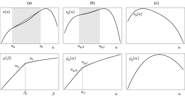
Figure 3: Schematic illustration of the effect of $g$ on the entropy and free energy functions. (Left) Initial entropy $s(u)$ and its corresponding free energy $\varphi(\beta)$ (see Figs. 1 and 2). (Middle) Modified entropy $s_{g}(u)$ having a smaller region of nonconcavity than $s(u)$, and its corresponding generalized free energy $\varphi_{g}(\alpha)$. (Right) A modified entropy $s_{g}(u)$ rendered fully concave by $g$; its corresponding generalized free energy $\varphi_{g}(\alpha)$ is everywhere differentiable.

We close our discussion of thermodynamic nonequivalence of ensembles by stating the generalization of Theorem 2. We omit the proof of this generalization as it follows directly from well-known properties of LF transforms and a straightforward generalization of well-known results about the equilibrium properties of the canonical ensemble.

Theorem 4.

Let $\varphi_{g}(\beta)$ denote the generalized free energy function defined in (13).

(a) If $\varphi_{g}$ is differentiable at $\alpha$, then

$$s(u_{g,\alpha}) = \varphi_{g}^{*}(u_{g,\alpha})+g(u_{g,\alpha})$$ (24)

$$= \alpha u_{g,\alpha}-\varphi_{g}(\alpha)+g(u_{g,\alpha}),$$

where $u_{g,\alpha}=\varphi_{g}^{\prime}(\alpha)$ represents the equilibrium value of $h$ in the generalized canonical ensemble with parameters $\alpha$ and $g$.

(b) if $\varphi_{g}$ is everywhere differentiable, then $s=\varphi_{g}^{*}+g$ for all $u$ in the range of $h$.

The implications of this theorem are illustrated in Fig. 3, which shows the plots of different entropy and free energy functions resulting from different choices for the function $g$. This figure depicts three possible scenarios:

(a) The original nonconcave entropy function $s(u)$ and its associated nondifferentiable free energy function $\varphi(\beta)$ for $g=0$. Recall in this case that the extent of the nonconcave region of $s(u)$ is equal to the latent heat associated with the nondifferentiable point of $\varphi(\beta)$; see Fig. 3.

(b) The modified entropy function $s_{g}(u)$ resulting from this choice of $g$ has a smaller region of nonconcavity than $s(u)$, which is to say that

$$\Delta u_{g}=u_{g,h}-u_{g,l}<\Delta u.$$ (25)

From the point of view of the generalized canonical ensemble, we have

$$\Delta u_{g}=\varphi_{g}^{\prime}(\alpha_{c}-0)-\varphi_{g}^{\prime}(\alpha_{c}+0),$$ (26)

and so we see that this choice of $g$ brings, in effect, the left- and right- derivative of $\varphi_{g}$ at $\alpha_{c}$ closer to one another compared to the case where $g=0$. In other words, this choice of $g$ has the effect of “inhibiting” the first-order phase transition of the canonical ensemble.

(c) There is a function $g$ that makes $s_{g}(u)$ strictly concave everywhere. In this case, $\varphi_{g}(\beta)$ is everywhere differentiable, which means that the first-order phase transition of the canonical ensemble has been completely obliterated. Thus, by varying $\alpha$, it is now possible to “scan” with $u_{g,\alpha}$ any values of the mean Hamiltonian $h$, which is a formal way to say that the generalized canonical ensemble can be used to access any particular mean energy value of the microcanonical ensemble, and so that both ensembles are equivalent.

IV Macrostate nonequivalence of ensembles

Just as the thermodynamic properties of systems can generally be related to their macrostates equilibrium properties, it is possible to define the equivalence or nonequivalence of the microcanonical and canonical ensembles at the macrostate level and relate this level to the thermodynamic level of nonequivalent ensembles described earlier. This was done recently by Ellis, Haven and Turkington Ellis et al. (2000). A full discussion of the results derived by these authors would fill too much space; we will limit ourselves here to present a summary version of the most important results found in Ref. Ellis et al. (2000) and then present generalizations of these results which are obtained by replacing the canonical ensemble with the generalized canonical ensemble Costeniuc et al. (2004b).

We first recall the basis for defining nonequivalent ensembles at the macrostate level. Given a macrostate or order parameter $m$, we proceed to calculate the equilibrium, that is, most probable values of $m$ in the microcanonical and canonical ensembles as a function of the mean energy $u$ and inverse temperature $\beta$, respectively. Let us denote the first set of microcanonical equilibrium values of $m$ parameterized as a function of $u$ by $\mathcal{E}^{u}$ and the second set of canonical equilibrium values parameterized as a function of $\beta$ by $\mathcal{E}_{\beta}$. By comparing these sets, we then define the following. On the one hand, we say that the microcanonical and canonical ensembles are equivalent at the macrostate level whenever, for a given $u$, there exists $\beta$ such that $\mathcal{E}^{u}=\mathcal{E}_{\beta}$. On the other hand, we say that the two ensembles are nonequivalent at the macrostate level if for a given $u$, there is no overlap between $\mathcal{E}^{u}$ and all possible sets $\mathcal{E}_{\beta}$, that is, mathematically if $\mathcal{E}^{u}\cap\mathcal{E}_{\beta}=\emptyset$ for all $\beta$.

These definitions of the macrostate level of equivalent and nonequivalent ensembles can be found implicitly in the work of Eyink and Spohn Eyink and Spohn (1993). They are stated explicitly in the comprehensive study of Ellis, Haven and Turkington Ellis et al. (2000), who have proved that the microcanonical and canonical ensembles are equivalent (resp., nonequivalent) at the macrostate level when they are equivalent (resp., nonequivalent) at the thermodynamic level. The main assumption underlying their work is that the mean Hamiltonian function $h(\omega)$ can be expressed as a function of the macrostate variable $m$ in the asymptotic limit where $n\rightarrow\infty$. A summary of their main results is presented next; see Ref. Ellis et al. (2000) for more complete and general results.

Theorem 5.

We say that $s$ admits a strict supporting line at $u$ if there exists $\beta$ such that $s(v)<s(u)+\beta(v-u)$ for all $v\neq u$.

(a) If $s$ admits a strict supporting line at $u$, then $\mathcal{E}^{u}=\mathcal{E}_{\beta}$ for some $\beta\in\mathbb{R}$, which equals $s^{\prime}(u)$ if $s$ is differentiable at $u$.

(b) If $s$ admits no supporting line at $u$, that is, equivalently, if $s(u)\neq s^{**}(u)$, then $\mathcal{E}^{u}\cap\mathcal{E}_{\beta}=\emptyset$ for all $\beta\in\mathbb{R}$.

The first case corresponds, as was stated above, to macrostate equivalence of ensembles, whereas the second corresponds to macrostate nonequivalence of ensembles. There is a third possible relationship that we omit from our analysis because of too many technicalities involved: it is referred to as partial equivalence and arises when $s$ possesses a non-strict supporting line at $u$, that is, a supporting line that touches the graph of $s(u)$ at more than one point Ellis et al. (2000).

Our next result is the generalization of Theorem 5 about macrostate equivalence and nonequivalence of ensembles. It shows, in analogy with the thermodynamic level, that the microcanonical properties of a system can be calculated from the point of view of the generalized canonical ensemble when the canonical ensemble cannot be used for that goal.

Theorem 6.

Let $s_{g}(u)=s(u)-g(u)$, where $g(u)$ is any continuous function of the mean energy $u$, and let $\mathcal{E}_{g,\alpha}$ denote the set of equilibrium values of the macrostate $m$ in the generalized canonical ensemble with function $g$ and parameter $\alpha$.

(a) If $s_{g}$ admits a strict supporting line at $u$, then $\mathcal{E}^{u}=\mathcal{E}_{g,\alpha}$ for some $\alpha\in\mathbb{R}$, which equals $s_{g}^{\prime}(u)$ if $s_{g}$ is differentiable at $u$.

(b) If $s_{g}$ does not admit a supporting line at $u$, that is, equivalently, if $s_{g}(u)\neq s_{g}^{**}(u)$, then $\mathcal{E}^{u}\cap\mathcal{E}_{g,\alpha}=\emptyset$ for all $\alpha\in\mathbb{R}$.

Proof.

For the purpose of proving this result, we define a generalized microcanonical ensemble by changing the Lebesgue measure $\mu(\omega)=d\omega$, which underlies the definition of the microcanonical ensemble, to the measure

$$\mu_{g}(\omega)=e^{-ng(h(\omega))}d\omega.$$ (27)

As mentioned before, the extra factor $e^{-ng(h(\omega))}$ modifies the microcanonical entropy $s(u)$ to $s_{g}(u)$ as shown in (19); however, and this is a crucial observation, it leaves all the macrostate equilibrium properties of the microcanonical ensemble unchanged because all the microstates that have the same mean energy still have the same weight. This implies that the generalized microcanonical ensemble is, by construction, always equivalent to the microcanonical ensemble at the macrostate level. That is to say, if $\mathcal{E}_{g}^{u}$ denotes the set of equilibrium values of the macrostate $m$ with respect to the generalized microcanonical ensemble with mean energy $u$ and function $g$, then $\mathcal{E}_{g}^{u}=\mathcal{E}^{u}$ for all $u$ and all $g$.

Next we observe that the supporting line properties of $s_{g}(u)$ determine whether the generalized microcanonical and generalized canonical ensembles are equivalent or not, just as the supporting line properties of $s(u)$ determine whether or not the standard microcanonical and standard canonical ensembles are equivalent; to be sure, compare equations (7) and (17).

With these two observations in hand, we are now ready to prove equivalence and nonequivalence results between $\mathcal{E}^{u}$ and $\mathcal{E}_{g,\alpha}$. Indeed, all we have to do is to use the equivalence and nonequivalence results of Theorem 5 to first derive equivalence and nonequivalence results about $\mathcal{E}_{g}^{u}$ and $\mathcal{E}_{g,\alpha}$, and then transform these to equivalence and nonequivalence results between $\mathcal{E}^{u}$and $\mathcal{E}_{g,\alpha}$ using the fact that $\mathcal{E}^{u}=\mathcal{E}_{g}^{u}$ for all $u$ and any choice of $g$. To prove Part (a), for example, we reason as follows. If $s_{g}$ admits a strict supporting line at $u$, then $\mathcal{E}_{g}^{u}=\mathcal{E}_{g,\alpha}$ for some $\alpha\in\mathbb{R}$. But since $\mathcal{E}_{g}^{u}=\mathcal{E}^{u}$ for all $u$ and any $g$, we obtain $\mathcal{E}^{u}=\mathcal{E}_{g,\alpha}$ for the same value of $\alpha$. Part (b) is proved similarly. If $s_{g}$ admits no supporting line at $u$, that is, if $s_{g}(u)\neq s_{g}^{**}(u)$, then $\mathcal{E}_{g}^{u}\cap\mathcal{E}_{g,\alpha}=\emptyset$ for all $\alpha\in\mathbb{R}$. Using again the equality $\mathcal{E}_{g}^{u}=\mathcal{E}^{u}$, we thus obtain $\mathcal{E}^{u}\cap\mathcal{E}_{g,\alpha}=\emptyset$ for all $\alpha\in\mathbb{R}$. ∎

V Gaussian ensemble

The choice $g(u)=\gamma u^{2}$ defines an interesting form of the generalized canonical ensemble that was introduced more than a decade ago by Hetherington Hetherington (1987) under the name of Gaussian ensemble; see also Refs. Stump and Hetherington (1987); Challa and Hetherington (1988a, b); Kiessling and Lebowitz (1997); Johal et al. (2003). Many properties of this ensemble were studied by Challa and Hetherington Challa and Hetherington (1988a, b) who showed, among other things, that the Gaussian ensemble can be thought of as arising when a sample system is put in contact with a finite heat reservoir. From this point of view, the Gaussian ensemble can be thought of as a kind of “bridge ensemble” that interpolates between the microcanonical ensemble, whose definition involves no reservoir, and the canonical ensemble, whose definition involves an infinite reservoir.

The results presented in this paper imply a somewhat different interpretation of the Gaussian ensemble. They show that the Gaussian ensemble can in fact be made equivalent with the microcanonical ensemble, in the thermodynamic limit, when the canonical ensemble cannot. A trivial implication of this is that the Gaussian ensemble can also be made equivalent with both the microcanonical and canonical ensembles if these are already equivalent. The precise formulation of these equivalence results is contained in Theorems 3 and 6 in which $s_{g}(u)$ takes the form $s_{\gamma}(u)=s(u)-\gamma u^{2}$.

In the specific case of the Gaussian ensemble, these results can be rephrased in a more geometric fashion using the fact that a supporting line condition for $s_{\gamma}$ at $u$ is equivalent to a supporting parabola condition for $s$ at $u$. To see this, we need to substitute the expression of $s_{\gamma}(u)$ and $\alpha=s_{\gamma}^{\prime}(u)=s^{\prime}(u)-2\gamma u$ in the definition of the supporting line to obtain

$$s(v)\leq s(u)+\alpha(v-u)+\gamma(v-u)^{2}$$ (28)

for all $v$. We assume at this point that $s_{\gamma}$, and therefore $s$, are differentiable functions at $u$. The right-hand side of this inequality represents the equation of a parabola that touches the graph of $s$ at $u$ and lies above that graph at all other points (Fig. 4); hence the term supporting parabola. As a result of this observation, we then have the following: if $s$ admits a supporting parabola at $u$ (Fig. 4), then

$$s(u) = \varphi_{\gamma}^{*}(u)+\gamma u^{2}$$ (29)

$$= \inf_{\alpha}\{\alpha u-\varphi_{\gamma}(\alpha)\}+\gamma u^{2};$$

otherwise the above equation is not valid. A macrostate extension of this result can be formulated in the same way by transforming the supporting line condition for $s_{\gamma}$ in Theorem 6 by a supporting parabola condition for $s(u)$.

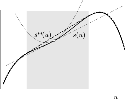
Figure 4: Example of a point of $s(u)$ which does not admit a supporting line but admits a supporting parabola. Such a point is accessible to the Gaussian ensemble but not to the canonical ensemble.

The advantage of using supporting parabola instead of supporting lines is that many properties of the Gaussian ensemble can be proved in a simple, geometric way. For example, it is clear that since $s(u)$ can possess a supporting parabola while not possessing a supporting line (Fig. 4), the Gaussian ensemble does indeed go beyond the standard canonical ensemble. Moreover, the range of nonconcavity of $s_{g}(u)$ should shrink as one chooses larger and larger values of $\gamma$. From this last observation, it should be expected that a single (finite) value of $\gamma$ can in fact be used to achieve equivalence between the Gaussian and microcanonical ensembles for all value $u$ in the range of $h$, provided that (i) $\gamma$ assumes a large enough value, basically greater that the largest second derivative of $s(u)$; (ii) that the graph of $s(u)$ contains no corners, that is, points where the derivative of $s(u)$ jumps and where $s^{\prime\prime}(u)$ is undefined; see Ref. Costeniuc et al. (2004b) for details.

The second point implies physically that the Gaussian ensemble with $\gamma<\infty$ cannot be applied at points of first-order phase transitions in the microcanonical ensemble. Such points, however, can be dealt with within the Gaussian ensemble by letting $\gamma\rightarrow\infty$, as we shall show in a forthcoming paper . With the proviso that the limit $\gamma\rightarrow\infty$ may have to be taken, we can then conclude that the Gaussian ensemble is a universal ensemble: in theory, it can recover any shape of microcanonical entropy function through Eq.(29), which means that it can achieve equivalence with the microcanonical ensemble for any system.

VI Conclusion

In this paper we have studied a generalization of the canonical ensemble which can be used to assess the microcanonical equilibrium properties of a system when the canonical ensemble is unavailing in that respect because of the presence of nonconcave anomalies in the microcanonical entropy function. Starting with the supporting properties of the microcanonical entropy, which are known to determine the equivalence and nonequivalence of the microcanonical and canonical ensembles, we have demonstrated how these properties can be extended at the level of a modified form of the microcanonical entropy to determine whether the microcanonical and generalized canonical ensembles are equivalent or not. Equivalence-of-ensembles conditions for these two ensembles were also given in terms of a generalized form of the canonical free energy. Finally, we have discussed the case of the Gaussian ensemble, a statistical-mechanical ensemble introduced some time ago by Hetherington, which arises here as a specific instance of our generalized canonical ensemble. For the Gaussian ensemble, results establishing the equivalence and nonequivalence with the microcanonical ensemble were given in terms of supporting parabolas.

In forthcoming papers, we will present applications of the generalized canonical ensemble for two simple spin models which are known to possess a nonconcave microcanonical entropy function. The first one is the Curie-Weiss-Potts model studied in Refs. Ispolatov and Cohen (2000); Costeniuc et al. (2004a); the second is the block spin model studied in Refs. Touchette (2003, 2005).