Exactly solvable model of quantum diffusion

Abstract

We study the transport property of diffusion in a finite translationally invariant quantum subsystem described by a tight-binding Hamiltonian with a single energy band and interacting with its environment by a coupling in terms of correlation functions which are delta-correlated in space and time. For weak coupling, the time evolution of the subsystem density matrix is ruled by a quantum master equation of Lindblad type. Thanks to the invariance under spatial translations, we can apply the Bloch theorem to the subsystem density matrix and exactly diagonalize the time evolution superoperator to obtain the complete spectrum of its eigenvalues, which fully describe the relaxation to equilibrium. Above a critical coupling which is inversely proportional to the size of the subsystem, the spectrum at given wavenumber contains an isolated eigenvalue describing diffusion. The other eigenvalues rule the decay of the populations and quantum coherences with decay rates which are proportional to the intensity of the environmental noise. On the other hand, an analytical expression is obtained for the dispersion relation of diffusion. The diffusion coefficient is proportional to the square of the width of the energy band and inversely proportional to the intensity of the environmental noise because diffusion results from the perturbation of quantum tunneling by the environmental fluctuations in this model. Diffusion disappears below the critical coupling.

I Introduction

The diffusion of particles in a condensed phase is a fundamental transport process which is ubiquitous in natural phenomena. Since the pioneering work by Einstein in 1905, it is known that diffusion is related to conduction or mobility. Although diffusion has been extensively studied in classical systems, much less is known in quantum systems where the quantum effects can deeply affect the transport properties at low temperature. Yet, the theoretical understanding of quantum diffusion remains sparse and difficult because diffusion is an incoherent process very remote from the very coherent basic quantum dynamics.

The purpose of the present paper is to study a simple model of quantum diffusion in a system which possesses the property of being invariant under spatial translations. This property is a fundamental feature of systems sustaining transport processes such as diffusion or conduction. The translational invariance is at the basis of the early studies of electronic conduction based on the Boltzmann-Lorentz equation Ashcroft , and is also important in the polaron model Holstein . Motivated by the problem of dissipation in quantum macroscopic phenomena, models of quantum Brownian motion have been proposed and studied since the eighties Caldeira . In such models, one degree of freedom has a diffusive-like motion in an external potential which breaks the translational invariance. These models were later extended to the study of transport in spatially periodic potentials Schmid ; Fisher ; Weiss1 ; Weiss2 ; Weiss ; Egger ; Lebowitz1 ; Lebowitz2 ; Lebowitz3 . In these studies, attention was focused essentially on diffusion. In the present study, we intend to study the complete set of the relaxation modes in the system by obtaining all the eigenvalues of the time evolution superoperator. The complete diagonalization of the time evolution superoperator is accomplished by fully exploiting the translational invariance with Bloch’s theorem applied to the density matrices. This allows us to introduce in a rigorous way a wavenumber and to obtain the eigenvalues which gives the Liouvillian resonances as functions of the wavenumber. These resonances provides us with the characteristic times of the relaxation toward the thermodynamic equilibrium. The hydrodynamic mode of diffusion is one among the eigenstates associated with the Liouvillian resonances. This mode controls the long-time dynamics of the system. The other modes control the shorter time scales and are associated with decoherence. In the quantum model here studied, analytical expressions can be obtained in this way for the dispersion relation of diffusion and the other resonances.

We notice that translationally invariant models without coupling to the environment have recently been studied in such models as quantum graphs Barra quantum multibaker maps Dorfman , as well as quantum periodic Lorentz gases Knauf . These models describe the motion of a quantum particle in a spatially periodic potential. The energy spectrum of the particle is composed of energy bands so that the motion is ballistic on long-time scales. If the energy of the particle is distributed over many energy bands, the motion becomes semiclassical and diffusion may manifest itself as a transient behavior before the long-time ballistic motion. This has been remarkably demonstrated for the quantum multibaker map in Ref. Dorfman . In order for diffusion to persist up to arbitrarily long times, the quantum system must contain infinitely many degrees of freedom, for instance, by the coupling with some environment in the subsystem-plus-reservoir approach we adopt in the present paper.

The plan of the paper is the following. Our translationally invariant model is defined in Sec. II by weakly coupling a one-dimensional tight-binding Hamiltonian to a delta-correlated environment. The dynamics of this system is ruled by a Redfield quantum master equation Red ; Kampen ; KuboB2 ; Breuer ; GaspRed . The long-time evolution of the model can be studied in terms of the eigenvalues and the associated eigenstates of the Redfield superoperator, as explained in Sec. III. The eigenvalue problem is exactly solved for a finite chain in Sec. IV. The advantage of first taking a finite chain is that the total number of eigenvalues is known and we do not miss the part of the spectrum controlling decoherence. The Liouvillian spectrum of the infinite chain is thereafter obtained in Sec. V by taking the limit $N\to\infty$. Conclusions are drawn in Sec. VI.

II Defining the system

II.1 Subsystem

We consider a one-dimensional subsystem described by the following Hamiltonian

$$\hat{H}_{\rm s}=\left(\begin{array}[]{ccccccc}E_{0}&-A&0&0&\ldots&0&-A\\ -A&E_{0}&-A&0&\ldots&0&0\\ 0&-A&E_{0}&-A&&0&0\\ \vdots&&\ddots&\ddots&\ddots&&\vdots\\ 0&0&&-A&E_{0}&-A&0\\ 0&0&\ldots&0&-A&E_{0}&-A\\ -A&0&\ldots&0&0&-A&E_{0}\\ \end{array}\right)_{N\times N}$$ (8)

(9)

represented in the site basis ${|l\rangle}$, where $l$ takes the values $l=0,1,\ldots,N-1$. $N$ is the length of the chain. We have here chosen periodic (Born-van Karman) boundary conditions. This so-called tight-binding or Hückel Hamiltonian describes a process of quantum tunneling from site to site and is invariant under spatial translations.

The stationary Schrödinger equation of the tight-binding Hamiltonian is given by

$$\hat{H}_{\rm s}|k\rangle=\epsilon_{k}|k\rangle,$$ (10)

where the eigenvalues are

$$\epsilon_{k}=E_{0}-2A\cos k\frac{2\pi}{N}$$ (11)

and the eigenvectors

$$\langle l|k\rangle=\frac{1}{\sqrt{N}}{\rm e}^{ilk\frac{2\pi}{N}},$$ (12)

with $k=0,1,...,N-1$. Accordingly, the Hamiltonian (9) has an energy spectrum with a single energy band of width $4A$ and the motion of the particle would be purely ballistic without coupling to a fluctuating environment.

II.2 Coupling to the environment

Now, we suppose that the subsystem is coupled to a large environment. The Hamiltonian of the total system composed of the one-dimensional chain and its environment is given by

$$\hat{H}_{\rm tot}=\hat{H}_{\rm s}+\hat{H}_{\rm b}+\lambda\sum_{l}\hat{S}_{l}\hat{B}_{l}\;,$$ (13)

where $\hat{H}_{\rm b}$ is the environment Hamiltonian, $\hat{S}_{l}$ the subsystem coupling operators, $\hat{B}_{l}$ the environment coupling operators, and $\lambda$ the coupling parameter which measures the intensity of the interaction between the subsystem and its environment.

The dynamics of the total system is described by the von Neumann equation

$$\frac{d\hat{\rho}_{\rm tot}(t)}{dt}=\hat{\hat{{\cal L}}}_{\rm tot}\hat{\rho}_{\rm tot}(t)=-i[\hat{H}_{\rm tot},\hat{\rho}_{\rm tot}(t)],$$ (14)

where $\hat{\hat{{\cal L}}}_{\rm tot}$ is the Liouvillian superoperator of the total system. We adopt the convention that $\hbar=1$. The reduced dynamics for the density matrix $\hat{\rho}(t)={\rm Tr}_{\rm b}\hat{\rho}_{\rm tot}(t)$ of the subsystem is known to obey a Redfield quantum master equation for weak coupling to the environment Red ; Kampen ; KuboB2 ; Breuer ; GaspRed . This equation can be systematically derived from the complete von Neumann equation for the total system (14) by second-order perturbation theory so that

$$\frac{d\hat{\rho}(t)}{dt}={\rm Tr}_{\rm b}\hat{\hat{{\cal L}}}_{\rm tot}\hat{\rho}_{\rm tot}(t)\stackrel{{\scriptstyle\lambda\ll 1}}{{=}}\hat{\hat{{\cal L}}}_{\rm Red}(t)\hat{\rho}(t)+O(\lambda^{3}).$$ (15)

On time scales longer than the correlation time of the environment, the Redfield quantum master equation is Markovian and reads

$$\frac{d\hat{\rho}}{dt} = \hat{\hat{{\cal L}}}_{\rm Red}\hat{\rho}$$ (16)

$$= -i[\hat{H}_{\rm s},\hat{\rho}]+\lambda^{2}\sum_{l}(\hat{T}_{l}\hat{\rho}\hat{S}_{l}$$

$$+ \hat{S}_{l}^{\dagger}\hat{\rho}\hat{T}_{l}^{\dagger}-\hat{S}_{l}\hat{T}_{l}\hat{\rho}-\hat{\rho}\hat{T}_{l}^{\dagger}\hat{S}_{l}^{\dagger})+O(\lambda^{3}),$$

where $\hat{\hat{{\cal L}}}_{\rm Red}$ is the so-called Redfield superoperator and where

$$\hat{T}_{l}\equiv\sum_{l^{\prime}}\int_{0}^{\infty}d\tau\;C_{ll^{\prime}}(\tau)\;{\rm e}^{-{i}\hat{H}_{\rm s}\tau}\hat{S}_{l^{\prime}}\;{\rm e}^{i\hat{H}_{\rm s}\tau}.$$ (17)

The correlation function of the environment which contains all the necessary information to describe the coupling of the subsystem to its environment is given by

$$C_{ll^{\prime}}(\tau)={\rm Tr}_{\rm b}\hat{\rho}_{\rm b}^{\rm eq}{\rm e}^{i\hat{H}_{\rm b}\tau}\hat{B}_{l}{\rm e}^{-i\hat{H}_{\rm b}\tau}\hat{B}_{l^{\prime}}$$ (18)

where $\hat{\rho}_{\rm b}^{\rm eq}$ is the canonical equilibrium state of the environment.

The interaction of the subsystem with its environment is expressed in terms of the subsystem coupling operators which are projection operators on the site basis

$$\langle l|\hat{S}_{l^{\prime\prime}}|l^{\prime}\rangle=\delta_{ll^{\prime}}\;\delta_{ll^{\prime\prime}}\;.$$ (19)

They take the unit value if the particle is located on the site $l^{\prime\prime}$ and zero otherwise. These operators have the properties:

$$\hat{S}_{l}^{n}=\hat{S}_{l}\;,$$ (20)

for $n=2,3,...$ and

$$\sum_{l}\hat{S}_{l}=\hat{I}\;.$$ (21)

We now need to specify the environment operators by the choice of the environment correlation functions. We make two assumptions:
Assumption 1: The environment dynamics has a very fast evolution compared with the subsystem dynamics. Therefore, the environment correlation functions decay in time so fast with respect to the characteristic time scales of the subsystem evolution, that they can be assumed to be Dirac delta distributions in time.
Assumption 2: The environment has very short range spatial correlations, much shorter than the distance between two adjacent sites of the subsystem. Accordingly, the environment correlation functions decay in space so fast that they can be assumed to be given by Kronecker delta in space.
These two assumptions mean that each of the environmental fluctuations at the different subsystem sites are statistically independent. The environment correlation functions are thus given by

$$C_{ll^{\prime}}(\tau)=2\;Q\;\delta(\tau)\;\delta_{ll^{\prime}}\;,$$ (22)

where $Q$ is a real number. The operators (17) in the Redfield equation (16) therefore become

$$\hat{T}_{l}=Q\;\hat{S}_{l}\;.$$ (23)

It has been shown in Ref. Esposito that the form taken by the operator (23) can be physically justified when $\tau_{\rm th}\ll\tau_{\rm b}\ll\tau_{\rm s}$, where $\tau_{\rm th}=1/k_{\rm B}T$ is the thermal time, $\tau_{\rm b}$ the correlation time of the environment or bath, and $\tau_{\rm s}$ the subsystem characteristic time.

Because of the fast decay of the temporal and the spatial correlations (22) and the properties of the subsystem coupling operators (19), the Redfield equation we have to solve takes the form

$$\frac{d\hat{\rho}}{dt} = \hat{\hat{{\cal L}}}_{\rm Red}\hat{\rho}$$

$$= -i[\hat{H}_{\rm s},\hat{\rho}]$$

$$+\lambda^{2}Q\sum_{l}(2\hat{S}_{l}\hat{\rho}\hat{S}_{l}-\hat{S}_{l}^{2}\hat{\rho}-\hat{\rho}\hat{S}_{l}^{2})+O(\lambda^{3})\;.$$

It can easily be verified by projecting this equation onto the site basis that it is translationally invariant (shifting all the site indices appearing in the projected equation by a constant does not modify the equation). Furthermore, this equation preserves the complete positivity of the density matrix because it has the Lindblad form Lindblad which is the result of a coupling with delta correlation functions GaspRed . It should also be mentioned that Eq. (II.2) can be directly derived from the complete von Neumann equation for the total system (14) in the singular coupling limit Gorini ; Spohn80 .

III Diagonalizing the Redfield superoperator

The eigenvalues $s_{\nu}$ and associated eigenstates ${\hat{\rho}}^{\nu}$ of the Redfield superoperator are defined by

$$\hat{\hat{{\cal L}}}_{\rm Red}\;{\hat{\rho}}^{\nu}=s_{\nu}\;{\hat{\rho}}^{\nu},$$ (25)

where $\nu$ is a set of parameters labeling the eigenstates. Because the Redfield superoperator is not anti-Hermitian, its eigenvalues can be complex numbers with a nonzero real part. The eigenvalue problem of the Redfield superoperator is important because the time evolution of the quantum master equation can then be decomposed onto the basis of the eigenstates as

$$\hat{\rho}(t)={\rm e}^{\hat{\hat{{\cal L}}}_{\rm Red}t}\hat{\rho}(0)=\sum_{\nu=1}^{N^{2}}c_{\nu}(0)\;{\rm e}^{s_{\nu}t}\hat{\rho}^{\nu}.$$ (26)

The dynamics is therefore given by a linear superposition of exponential or oscillatory exponential functions. Since the reduced density matrix of the subsystem has $N^{2}$ elements, there is a total of $N^{2}$ eigenvalues and associated eigenstates.

III.1 Bloch theorem

Since the system is invariant under spatial translations, we can apply the Bloch theorem to the eigenstates of the Redfield superoperator. Thanks to this theorem, the state space of the superoperator can be decomposed into independent superoperators acting onto decoupled sectors associated with a given Bloch number, also called wavenumber Ashcroft .

We define the superoperator $\hat{\hat{{\cal T}}}_{a}$ of the spatial translation by $a$ sites along the system ($a$ is an integer) as

$$(\hat{\hat{{\cal T}}}_{a}\rho^{{\nu}})_{ll^{\prime}}=\rho^{{\nu}}_{l+a,l^{\prime}+a}\;,$$ (27)

where we use the notation $\langle l|\hat{\rho}|l^{\prime}\rangle=\rho_{ll^{\prime}}$. This superoperator has the group property

$$\hat{\hat{{\cal T}}}_{a}\hat{\hat{{\cal T}}}_{a^{\prime}}=\hat{\hat{{\cal T}}}_{a^{\prime}}\hat{\hat{{\cal T}}}_{a}=\hat{\hat{{\cal T}}}_{a+a^{\prime}}\;.$$ (28)

Because of the translational symmetry of the system, the translation superoperators commute with the Redfield superoperator

$$\left[\hat{\hat{{\cal T}}}_{a},\hat{\hat{{\cal L}}}_{\rm Red}\right]=0\;.$$ (29)

Therefore, the Redfield superoperator as well as the translation superoperators have a basis of common eigenstates. If $\tau(a)$ denotes the eigenvalues of the translation superoperator, we have that

$$\hat{\hat{{\cal T}}}_{a}\;{\hat{\rho}}^{{\nu}}=\tau(a)\;{\hat{\rho}}^{{\nu}}\;,$$ (30)

where, because of the unitarity of $\hat{\hat{{\cal T}}}_{a}$,

$$|\tau(a)|^{2}=1\;.$$ (31)

Equation (28) implies

$$\tau(a+a^{\prime})=\tau(a)\;\tau(a^{\prime})\;.$$ (32)

Because of Eqs. (31) and (32), we find that

$$\tau(a)={\rm e}^{iqa}\;,$$ (33)

where $q$ is the Bloch number or wavenumber, whereupon we get

$$\rho^{{\nu}}_{l+a,l^{\prime}+a}={\rm e}^{iqa}\rho^{{\nu}}_{ll^{\prime}}\;.$$ (34)

A useful consequence is that

$$\rho^{{\nu}}_{ll^{\prime}}={\rm e}^{iql}\rho^{{\nu}}_{0,l^{\prime}-l}\;.$$ (35)

In order to determine the allowed values of the Bloch number, we write by using Eq. (12) that

$$\rho^{\nu}_{ll^{\prime}}=\frac{1}{N}\sum_{k,k^{\prime}}\langle k|\hat{\rho}^{\nu}|k^{\prime}\rangle{\rm e}^{i(lk-l^{\prime}k^{\prime})\frac{2\pi}{N}}$$ (36)

and

$$\rho^{\nu}_{l+1,l^{\prime}+1} = \frac{1}{N}\sum_{k,k^{\prime}}\langle k|\hat{\rho}^{\nu}|k^{\prime}\rangle{\rm e}^{i(lk-l^{\prime}k^{\prime})\frac{2\pi}{N}}{\rm e}^{i(k-k^{\prime})\frac{2\pi}{N}}.$$ (37)

Because of Eq. (34), we also have

$$\rho^{\nu}_{l+1,l^{\prime}+1} = {\rm e}^{iq}\;\rho^{\nu}_{ll^{\prime}}\;.$$ (38)

Multiplying both sides of Eqs. (37) and (38) by $\langle l^{\prime}|k^{\prime\prime\prime}\rangle\langle k^{\prime\prime}|l\rangle$, taking the sum $\sum_{l,l^{\prime}}$ of it, and identifying them, we obtain

$${\rm e}^{iq}\langle k|\hat{\rho}^{\nu}|k^{\prime}\rangle={\rm e}^{i(k-k^{\prime})\frac{2\pi}{N}}\langle k|\hat{\rho}^{\nu}|k^{\prime}\rangle.$$ (39)

We can now notice that if $q\neq(k-k^{\prime})\frac{2\pi}{N}$, then $\langle k|\hat{\rho}^{\nu}|k^{\prime}\rangle=0$. Finally, using the periodicity

$$\rho_{l+N,l^{\prime}}^{{\nu}} = \rho_{ll^{\prime}}^{{\nu}}\;,$$ (40)

$$\rho_{l,l^{\prime}+N}^{{\nu}} = \rho_{ll^{\prime}}^{{\nu}}\;,$$ (41)

and Eq. (34), we find that the Bloch number takes the values

$$q=j\frac{2\pi}{N},\ \ \text{where}\ \ j=0,1,\ldots,N-1\;.$$ (42)

Consequently, the Redfield superoperator can be block-diagonalized into $N$ independent blocks, which each contains $N$ eigenvalues as we shall see in the following.

III.2 Simplifying the problem

The eigenvalue problem of the Redfield superoperator can be formulated in each sector labeled by a given wavenumber $q$. For this purpose, Eq. (25) with the explicit expression (II.2) of the Redfield superoperator is projected onto the site basis to get

$$s_{\nu}\rho^{\nu}_{ll^{\prime}} = -iA\left(-\rho^{\nu}_{l-1,l^{\prime}}-\rho^{\nu}_{l+1,l^{\prime}}+\rho^{\nu}_{l,l^{\prime}-1}+\rho^{\nu}_{l,l^{\prime}+1}\right)$$ (43)

$$+2\lambda^{2}Q\left(\delta_{ll^{\prime}}-1\right)\rho^{\nu}_{ll^{\prime}}\;.$$

Using Eq. (35) and replacing $l^{\prime}-l$ by $l$, we have

$$\left(s_{\nu}+2Q\lambda^{2}\right)\rho^{{\nu}}_{0l} = 2A\left(\sin\frac{q}{2}\right)\left({\rm e}^{-i\frac{q}{2}}\rho^{{\nu}}_{0,l+1}-{\rm e}^{i\frac{q}{2}}\rho^{{\nu}}_{0,l-1}\right)$$ (44)

$$+2Q\lambda^{2}\rho^{{\nu}}_{00}\;\delta_{0l}\;.$$

Making the change of variable

$$\rho^{{\nu}}_{0l}=i^{-l}{\rm e}^{i\frac{q}{2}l}f_{l}\;,$$ (45)

we obtain the simpler eigenvalue equation

$$\mu_{\nu}f_{l} = \delta_{0l}f_{l}-i\beta(f_{l-1}+f_{l+1})\;,$$ (46)

where

$$\mu_{\nu}=\frac{s_{\nu}}{2Q\lambda^{2}}+1\;,$$ (47)

and

$$\beta=\frac{A}{Q\lambda^{2}}\sin\frac{q}{2}\;.$$ (48)

IV Finite chain

IV.1 The eigenvalue problem

The expression (46) can be written in matrix form without the index ${\nu}$ to simplify the notation,

$$\mu\vec{f}=\hat{W}\vec{f}\;,$$ (49)

where $\mu$ denotes the eigenvalue, $\vec{f}=(f_{0},\ldots,f_{N-1})$ the eigenvector of size $N$, and $\hat{W}$ the following $N\times N$ matrix

$$\left(\begin{array}[]{ccccccccc}1&-i\beta&&&&&-i\beta i^{-N}{\rm e}^{iN\frac{q}{2}}\\ -i\beta&0&-i\beta&&&&\\ &-i\beta&0&-i\beta&&&\\ &&\ddots&\ddots&\ddots&&\\ &&&-i\beta&0&-i\beta&\\ &&&&-i\beta&0&-i\beta\\ -i\beta i^{N}{\rm e}^{-iN\frac{q}{2}}&&&&&-i\beta&0\\ \end{array}\right)$$ (57)

(58)

We look for eigenstates of the form

$$f_{l}=A{\rm e}^{i\theta l}+B{\rm e}^{-i\theta l}.$$ (59)

Solving Eq. (49) with (59) gives

• for $0<l<N-1$:

  $$\mu=-2i\;\beta\;\cos\theta\;,$$ (60)

• for $l=0$:

  $$(1-\mu)(A+B)-i\beta(A{\rm e}^{i\theta}+B{\rm e}^{-i\theta})$$

  $$-i\beta i^{-N}{\rm e}^{iN\frac{q}{2}}(A{\rm e}^{i\theta(N-1)}+B{\rm e}^{-i\theta(N-1)})=0\;,$$ (61)

• for $l=N-1$:

  $$A{\rm e}^{i\theta N}+B{\rm e}^{-i\theta N}-i^{N}{\rm e}^{-iN\frac{q}{2}}(A+B)=0\;.$$ (62)

Solving the homogeneous linear system of Eqs. (61) and (62) and replacing $\mu$ by (60), one gets the characteristic equation

$$2i\beta\sin\theta\left[R(q)-\cos\theta N\right]=\sin\theta N,$$ (63)

with

$$R(q)=\frac{1}{2}\left(i^{N}{\rm e}^{-iN\frac{q}{2}}+i^{-N}{\rm e}^{iN\frac{q}{2}}\right).$$ (64)

Using Eq. (42), we find:

for $$\;N\;\mbox{odd}:\qquad R(q_{j})=0\;,$$ (65)

for $$\;N=4I:\qquad R(q_{j})=(-1)^{j}\;,$$ (66)

for $$\;N=4I+2:\qquad R(q_{j})=-(-1)^{j}\;,$$ (67)

with $I$ integer. From now on, we shall speak of even (respectively odd) $q$, if $q$ corresponds to an even (respectively odd) integer $j$ in Eq. (42). Therefore, the characteristic equation (63) becomes

• for $N$ odd:

  $$2i\beta\sin\theta=-\tan\theta N\;;$$ (68)

• for $N=4I$ and $q$ even or for $N=4I+2$ and $q$ odd:
  either

  $$2i\beta\sin\theta = {\rm cotan}\frac{\theta N}{2}\;,$$ (69)

  or

  $$\cos\theta N = 1\;;$$ (70)

• for $N=4I$ and $q$ odd or for $N=4I+2$ and $q$ even:
  either

  $$2i\beta\sin\theta = -\tan\frac{\theta N}{2}\;,$$ (71)

  or

  $$\cos\theta N = -1\;.$$ (72)

We solve Eqs. (68)-(72) as follows.

IV.2 The diffusive eigenvalue $\mu^{(1)}$

We first look for an eigenvalue $\mu$ which is real and should correspond to a monotonic exponential decay. With this goal, we suppose that the angle $\theta$ is complex

$$\theta=\xi+i\eta\;,$$ (73)

so that the eigenvalue (60) becomes

$$\mu=-2i\beta\cos\theta=-2\beta\sin\xi\sinh\eta-2i\beta\cos\xi\cosh\eta\;.$$ (74)

This eigenvalue is real under the condition that $\cos\xi=0$ which is satisfied for

$$\xi=-\frac{\pi}{2}\;,$$ (75)

in which case

$$\mu=-2\;\beta\;\sinh\eta\;.$$ (76)

We notice that the condition $\cos\xi=0$ is also satisfied for $\xi=\frac{\pi}{2}$ but it can be shown that this other case leads to the same eigenvalue as (75). If we introduce the conditions (73) and (75) in Eqs. (68), (69), and (71), we get

• for $N$ odd:

  $$2\beta\cosh\eta=\coth N\eta\;;$$ (77)

• for $N=4I$ and $q$ even or for $N=4I+2$ and $q$ odd:
  

  $$2\beta\cosh\eta = \coth\frac{N\eta}{2}\;;$$ (78)

• for $N=4I$ and $q$ odd or for $N=4I+2$ and $q$ even:
  

  $$2\beta\cosh\eta = \tanh\frac{N\eta}{2}\;.$$ (79)

In the limit $N\to\infty$, the right-hand side of these equations tends to unity if a nonvanishing solution $\eta\neq 0$ exists. In this limit, this solution is thus given by

$$\eta_{0} = {\rm arccosh}\;\frac{1}{2\beta}\;,$$ (80)

which exists only if $\beta\leq\frac{1}{2}$. Because

$$\sinh\eta_{0} = \sqrt{\left(\frac{1}{2\beta}\right)^{2}-1}\;,$$ (81)

the corresponding eigenvalue should be

$$\mu_{0} = \sqrt{1-(2\beta)^{2}}\;.$$ (82)

However, for a finite chain with $N<\infty$, we expect a correction $\delta\eta$ to the solution $\eta=\eta_{0}+\delta\eta$. Replacing this correction in Eqs. (77), (78), and (79), we obtain by Taylor expansion that

• for $N$ odd:

  $$\delta\eta\simeq 2\;\frac{{\rm e}^{-2N{\rm arccosh}\;\frac{1}{2\beta}}}{\sqrt{1-(2\beta)^{2}}}\;;$$ (83)

• for $N=4I$ and $q$ even or for $N=4I+2$ and $q$ odd:

  $$\delta\eta\simeq 2\;\frac{{\rm e}^{-N{\rm arccosh}\;\frac{1}{2\beta}}}{\sqrt{1-(2\beta)^{2}}}\;;$$ (84)

• for $N=4I$ and $q$ odd or for $N=4I+2$ and $q$ even:

  $$\delta\eta\simeq-2\;\frac{{\rm e}^{-N{\rm arccosh}\;\frac{1}{2\beta}}}{\sqrt{1-(2\beta)^{2}}}\;;$$ (85)

up to corrections of $O(\delta\eta^{2})$. Using the expression (76), we finally obtain the eigenvalue

$$\mu^{(1)} = 2\beta\sinh\eta_{0}+2\beta\cosh\eta_{0}\;\delta\eta+O(\delta\eta^{2})$$ (86)

$$= \sqrt{1-(2\beta)^{2}}+\delta\eta+O(\delta\eta^{2})\;,$$

where $\delta\eta$ is respectively given by Eqs. (83), (84), and (85). Accordingly, the correction $\delta\eta$ to the eigenvalue decreases exponentially fast with the size $N$ of the chain.

Using Eqs. (47) and (48), we finally obtain the eigenvalue

$$s^{(1)} = 2Q\lambda^{2}(\mu^{(1)}-1)$$

$$= 2Q\lambda^{2}\sqrt{1-\left(\frac{2A}{Q\lambda^{2}}\sin\frac{q}{2}\right)^{2}}-2Q\lambda^{2}+O(\delta\eta)\;.$$

The eigenvalue $s^{(1)}=0$ corresponding to a vanishing wavenumber $q=0$ is always in the spectrum of the Redfield superoperator. The associated eigenstate describes the stationary equilibrium state. At low wavenumbers $q,\beta\to 0$, we recover the dispersion relation of diffusion

$$s^{(1)}=-Dq^{2}+O(q^{4})\;,$$ (88)

with the diffusion coefficient

$$D=\frac{A^{2}}{Q\lambda^{2}}\;,$$ (89)

which justifies calling $\mu^{(1)}$ or $s^{(1)}$ the diffusive eigenvalue.

We notice that the diffusive eigenvalue no longer exists beyond the critical value $\beta_{\rm c}=\frac{1}{2}$. Since the matrix (58) has a total of $N$ eigenvalues, we expect further nondiffusive eigenvalues in a number of $N-1$ for $\beta<\frac{1}{2}$ and $N$ for $\beta>\frac{1}{2}$, as confirmed in the following subsections.

IV.3 The eigenvalues $\mu^{(2)}$

Beside the diffusive eigenvalue, we expect eigenvalues corresponding to the chain-like structure of the matrix (58). To obtain these eigenvalues, we pose $\tan\chi=2i\beta\sin\theta$ so that Eqs. (68), (69), and (71) can be written respectively

$$\sin(\theta N+\chi)=0\;,$$ (90)

$$\cos\left(\frac{\theta N}{2}+\chi\right)=0\;,$$ (91)

$$\sin\left(\frac{\theta N}{2}+\chi\right)=0\;.$$ (92)

Therefore, we obtain

$$i\left(n\pi-\theta N\right) = {\rm arctanh}(-2\beta\sin\theta)\;,$$ (93)

$$i\left(n\pi+\frac{\pi}{2}-\frac{\theta N}{2}\right) = {\rm arctanh}(-2\beta\sin\theta)\;,$$ (94)

$$i\left(n\pi-\frac{\theta N}{2}\right) = {\rm arctanh}(-2\beta\sin\theta)\;.$$ (95)

We now expand ${\rm arctanh}(-2\beta\sin\theta)$ around $\beta=0$:

$${\rm arctanh}(-2\beta\sin\theta)\stackrel{{\scriptstyle\beta\to 0}}{{=}}-2\beta\sin\theta-\frac{8}{3}\beta^{3}\sin^{3}\theta+O(\beta^{5})\;.$$

(96)

If $\beta=0$, the solutions of Eqs. (93), (94), and (95) are respectively given by

$$\theta_{0} = \frac{n\pi}{N},\ \ \text{where}\ \ n=1,2,\ldots,N-1,$$ (97)

$$\theta_{0} = \frac{(2n+1)\pi}{N},\ \ \text{where}\ \ n=0,1,\ldots,\frac{N}{2}-1,$$ (98)

$$\theta_{0} = \frac{2n\pi}{N},\ \ \text{where}\ \ n=1,2,\ldots,\frac{N}{2}-1,$$ (99)

Notice that $n=0$ is rejected in Eqs. (97) and (99). It is due to the fact that $\theta=0$ does not correspond to an eigenvector because it can be seen that $f_{l}=A+B\neq 0$ in Eq. (59) cannot be an eigenvector of Eq. (58).

Using the expansion (96) in Eqs. (93), (94) and (95) with $\theta=\theta_{0}+\delta\theta$, we find

$$\delta\theta\stackrel{{\scriptstyle\beta\to 0}}{{=}} -\frac{i2\beta}{M}\sin\theta_{0}-\frac{i8\beta^{3}}{3M}\sin^{3}\theta_{0}$$ (100)

$$+O\left(i\frac{\beta^{5}}{M}\right)+O\left(\frac{\beta^{2}}{M^{2}}\right),$$

where $M=N$ for Eq. (93) and $M=\frac{N}{2}$ for Eqs. (94) and (95). The eigenvalue (60) is now given by the expansion

$$\mu = -2i\beta\cos(\theta_{0}+\delta\theta)$$ (101)

$$\stackrel{{\scriptstyle\delta\theta\to 0}}{{=}} -2i\beta\cos\theta_{0}+2i\beta\sin\theta_{0}\;\delta\theta$$

$$+i\beta\cos\theta_{0}\;\delta\theta^{2}+O(\delta\theta^{3}).$$

Using Eq. (100) in (101) gives

$$\mu^{(2)} \stackrel{{\scriptstyle\beta\to 0}}{{=}} -2i\beta\cos\theta_{0}+O\left(i\frac{\beta^{3}}{M^{2}}\right)$$

$$+\frac{4\beta^{2}}{M}\sin^{2}\theta_{0}+\frac{16\beta^{4}}{3M}\sin^{4}\theta_{0}+O\left(\frac{\beta^{6}}{M}\right)\;.$$

Consequently, we have

• for $N$ odd, using Eq. (LABEL:spec2aad) with (97):

  $$\mu^{(2)} \stackrel{{\scriptstyle\beta\to 0}}{{=}} -2i\beta\cos\frac{n\pi}{N}+\frac{4\beta^{2}}{N}\sin^{2}\frac{n\pi}{N}+\frac{16\beta^{4}}{3N}\sin^{4}\frac{n\pi}{N},$$ (103)

  $$\text{where}\ \ n=1,2,\ldots,N-1\;;$$

• for $N=4I$ and $q$ even or for $N=4I+2$ and $q$ odd, using Eq. (LABEL:spec2aad) with (98):

  $$\mu^{(2)} \stackrel{{\scriptstyle\beta\to 0}}{{=}} -2i\beta\cos\frac{(2n+1)\pi}{N}$$ (104)

  $$+\frac{8\beta^{2}}{N}\sin^{2}\frac{(2n+1)\pi}{N}+\frac{32\beta^{4}}{3N}\sin^{4}\frac{(2n+1)\pi}{N},$$

  $$\text{where}\ \ n=0,1,\ldots,\frac{N}{2}-1\;;$$

• for $N=4I$ and $q$ odd or for $N=4I+2$ and $q$ even, using Eq. (LABEL:spec2aad) with (99):

  $$\mu^{(2)} \stackrel{{\scriptstyle\beta\to 0}}{{=}} -2i\beta\cos\frac{2n\pi}{N}+\frac{8\beta^{2}}{N}\sin^{2}\frac{2n\pi}{N}+\frac{32\beta^{4}}{3N}\sin^{4}\frac{2n\pi}{N},$$ (105)

  $$\text{where}\ \ n=1,2,\ldots,\frac{N}{2}-1\;.$$

IV.4 The eigenvalues $\mu^{(3)}$

The solutions of Eq. (70) are simply given by

$$\theta=\frac{2n\pi}{N},\ \ \text{where}\ \ n=1,2,\ldots,\frac{N}{2}-1\;.$$ (106)

We reject $n=0$ and $n=\frac{N}{2}$ because the corresponding eigenvector does not exist in these cases. Similarly, the solutions of Eq. (72) are given by

$$\theta=\frac{(2n+1)\pi}{N},\ \ \text{where}\ \ n=0,1,\ldots,\frac{N}{2}-1\;.$$ (107)

Consequently, we have the further eigenvalues:

• for $N=4I$ and $q$ even or for $N=4I+2$ and $q$ odd, using Eq. (60) with (106):

  $$\mu^{(3)} = -2i\beta\cos\left(\frac{2n\pi}{N}\right)\;,\ \ \text{where}\ \ n=1,2,\ldots,\frac{N}{2}-1\;;$$

• for $N=4I$ and $q$ odd or for $N=4I+2$ and $q$ even, using Eq. (60) with (107):

  $$\mu^{(3)} = -2i\beta\cos\left(\frac{(2n+1)\pi}{N}\right),$$ (109)

  $$\text{where}\ \ n=0,1,\ldots,\frac{N}{2}-1\;.$$

IV.5 The eigenvalues $\mu^{(4)}$

An important observation is that, for $\beta<\frac{1}{2}$, the expansion (96) which implies $2\beta\sin\theta<1$ is satisfied everywhere, i.e., for all the values of $\theta$ and therefore for all the eigenvalues. However, for $\beta>\frac{1}{2}$, the Taylor expansion around $\beta=0$ in Eq. (96) is only valid if $2\beta\sin\theta<1$. Therefore, a transition zone exists around $\sin\theta\simeq 1/(2\beta)$. According to Eq. (60), this transition corresponds to the critical value of the eigenvalue given by

$$\mu_{\rm c} = \pm i\sqrt{(2\beta)^{2}-1}\;.$$ (110)

Therefore, for $\beta>\frac{1}{2}$, the expansion (96) around $\beta=0$ is only valid if $|\mu|>|\mu_{\rm c}|$. For $|\mu|<|\mu_{\rm c}|$, we should instead consider the asymptotic expansion of ${\rm arctanh}(-2\beta\sin\theta)$ around $\beta=\infty$:

$${\rm arctanh}(-2\beta\sin\theta) \stackrel{{\scriptstyle\beta\to\infty}}{{=}} i\frac{\pi}{2}-\frac{1}{2\beta\sin\theta}-\frac{1}{24\beta^{3}\sin^{3}\theta}$$

$$-\frac{1}{160\beta^{5}\sin^{5}\theta}+O\left(\frac{1}{\beta^{7}}\right)\;,$$

which leads to another family of eigenvalues existing for $\beta>\frac{1}{2}$.

If $\beta\to\infty$, the solutions of Eqs. (93), (94) and (95) are respectively given by

$$\theta_{0} = \frac{(n+\frac{1}{2})\pi}{N},\ \ \text{where}\ \ n=0,1,\ldots,N-1\,,$$ (112)

$$\theta_{0} = \frac{2n\pi}{N},\ \ \text{where}\ \ n=1,2,\ldots,\frac{N}{2}-1\,,$$ (113)

$$\theta_{0} = \frac{(2n+1)\pi}{N},\ \ \text{where}\ \ n=0,1,\ldots,\frac{N}{2}-1.$$ (114)

Because of the condition $|\mu|<|\mu_{\rm c}|$ with the critical values (110), we should only consider the angles in the interval $\theta_{0,{\rm c}}<\theta_{0}<\pi-\theta_{0,{\rm c}}$ with

$$\theta_{0,{\rm c}} = \arcsin\frac{1}{2\beta}\;,$$ (115)

so that the integer $n$ in Eqs. (112), (113), and (114) is restricted to take the intermediate values $n_{\rm min}<n<n_{\rm max}$ which do not reach the extreme values.

Using the expansion (LABEL:spec2aaa) in Eqs. (93), (94), and (95) with $\theta=\theta_{0}+\delta\theta$, we find

$$\delta\theta \stackrel{{\scriptstyle\beta\to\infty}}{{=}} -\frac{i}{2\beta M\sin\theta_{0}}-\frac{i}{24\beta^{3}M\sin^{3}\theta_{0}}-\frac{i}{160\beta^{5}M\sin^{5}\theta_{0}}$$ (116)

$$+O\left(\frac{i}{\beta^{7}M}\right)+O\left(\frac{1}{\beta^{2}M^{2}}\right)\;,$$

where $M=N$ for Eq. (93) and $M=\frac{N}{2}$ for Eqs. (94) and (95).

Using Eq. (116) in (101) gives

$$\mu^{(4)} \stackrel{{\scriptstyle\beta\to\infty}}{{=}} -2i\beta\cos\theta_{0}+\frac{1}{M}\left(1+\frac{1}{12\beta^{2}\sin^{2}\theta_{0}}\right.$$

$$\left.+\frac{1}{80\beta^{4}\sin^{4}\theta_{0}}\right)+O\left(\frac{1}{\beta^{6}M}\right)+O\left(\frac{i}{\beta M^{2}}\right)\;.$$

Consequently, we have

• for $N$ odd, using Eq. (LABEL:spec2aae) with (112):

  $$\mu^{(4)} \stackrel{{\scriptstyle\beta\to\infty}}{{=}} -2i\beta\cos\frac{(n+\frac{1}{2})\pi}{N}+\frac{1}{N}\left(1+\frac{1}{12\beta^{2}\sin^{2}\frac{(n+\frac{1}{2})\pi}{N}}\right.$$ (118)

  $$\left.+\frac{1}{80\beta^{4}\sin^{4}\frac{(n+\frac{1}{2})\pi}{N}}\right),$$

  $$\text{where}\ \ n=0,1,\ldots,N-1\;;$$

• for $N=4I$ and $q$ even or for $N=4I+2$ and $q$ odd, using Eq. (LABEL:spec2aae) with (113):

  $$\mu^{(4)} \stackrel{{\scriptstyle\beta\to\infty}}{{=}} -2i\beta\cos\frac{2n\pi}{N}$$ (119)

  $$+\frac{2}{N}\left(1+\frac{1}{12\beta^{2}\sin^{2}\frac{2n\pi}{N}}+\frac{1}{80\beta^{4}\sin^{4}\frac{2n\pi}{N}}\right),$$

  $$\text{where}\ \ n=1,2,\ldots,\frac{N}{2}-1\;;$$

• for $N=4I$ and $q$ odd or for $N=4I+2$ and $q$ even, using Eq. (LABEL:spec2aae) with (114):

  $$\mu^{(4)} \stackrel{{\scriptstyle\beta\to\infty}}{{=}} -2i\beta\cos\frac{(2n+1)\pi}{N}$$ (120)

  $$+\frac{2}{N}\left(1+\frac{1}{12\beta^{2}\sin^{2}\frac{(2n+1)\pi}{N}}\right.$$

  $$\left.+\frac{1}{80\beta^{4}\sin^{4}\frac{(2n+1)\pi}{N}}\right),$$

  $$\text{where}\ \ n=0,1,\ldots,\frac{N}{2}-1\;;$$

with the aforementioned restriction on the values of the integer $n$.

IV.6 The eigenvalues $\mu^{(5)}$

For $N=4I$ and $q$ even or $N=4I+2$ and $q$ odd, two special eigenvalues exist in the limit $\beta\to\infty$ around $\theta_{0}=0$ and $\theta_{0}=\pi$. They can be obtained by taking $\theta=\theta_{0}+\delta\theta$ and directly solving Eq. (69) to get in both cases

$$\delta\theta^{2}\stackrel{{\scriptstyle\beta\to\infty}}{{=}}\frac{1}{i\beta N}+O\left(\frac{1}{\beta^{2}}\right)\;.$$ (121)

Inserting in Eq. (101), we obtain

$$\mu^{(5)} \stackrel{{\scriptstyle\beta\to\infty}}{{=}} \mp 2i\beta+\frac{1}{N}+O\left(\frac{1}{\beta}\right)\;.$$ (122)

IV.7 Description of the spectrum

Rewriting the eigenvalues (60) of the Redfield superoperator with their explicit dependence in terms of Eq. (48), we get

$$\mu_{\nu}=\mu_{q\theta}=-2i\beta\cos\theta=-2i\frac{A}{Q\lambda^{2}}\left(\sin\frac{q}{2}\right)\cos\theta\;,$$ (123)

where $\nu$ can take $N^{2}$ different values because $q$ and $\theta$ take $N$ values each. Remembering that according to Eq. (47)

$$s_{\nu}=s_{q\theta}=2Q\lambda^{2}(\mu_{q\theta}-1),$$ (124)

we conclude that we have found in this section all the eigenvalues of the Redfield superoperator. We list them in Tables 1 and 2 according to the parameter regime in which they hold.

We now discuss the main features of the spectrum when the different physical parameters are varied. This discussion is based on our analytical results for the eigenvalues and on the comparison between these results and the eigenvalues obtained by numerical diagonalization of the Redfield superoperator. Since the eigenvalues $\mu_{q\theta}$ are related to the Redfield superoperator eigenvalues $s_{q\theta}$ by Eq. (124), we notice that all the eigenvalues of the complete spectrum always satisfy $0\leq{\rm Re}\;\mu_{q\theta}\leq 1$ or, equivalently, $-2Q\lambda^{2}\leq{\rm Re}\;s_{q\theta}\leq 0$. The imaginary part of $s_{q\theta}$ is simply proportional by a factor $2Q\lambda^{2}$ to the imaginary part of $\mu_{q\theta}$.

We start by studying the $N$ eigenvalues $\mu_{q\theta}$ obtained by fixing the wavenumber $q$ (even or odd) and varying $\theta$. For given physical parameters ($A$, $\lambda$, $Q$, $N$), fixing $q$ is equivalent to fixing $\beta$.

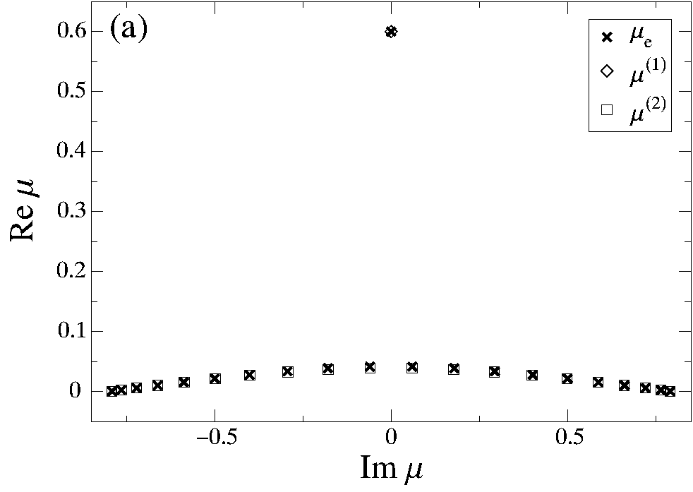
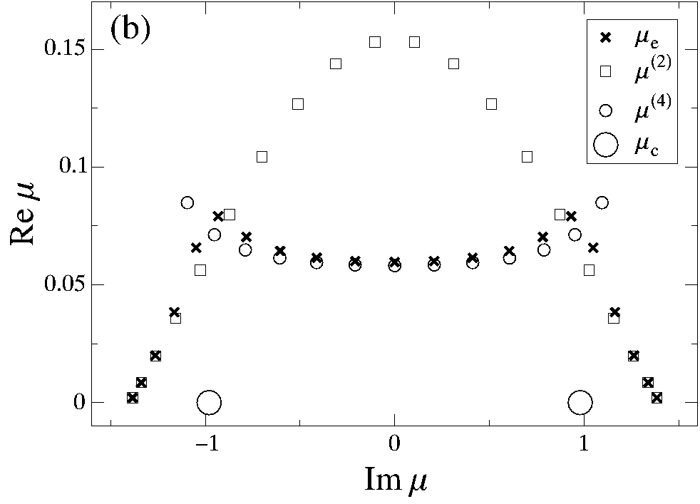
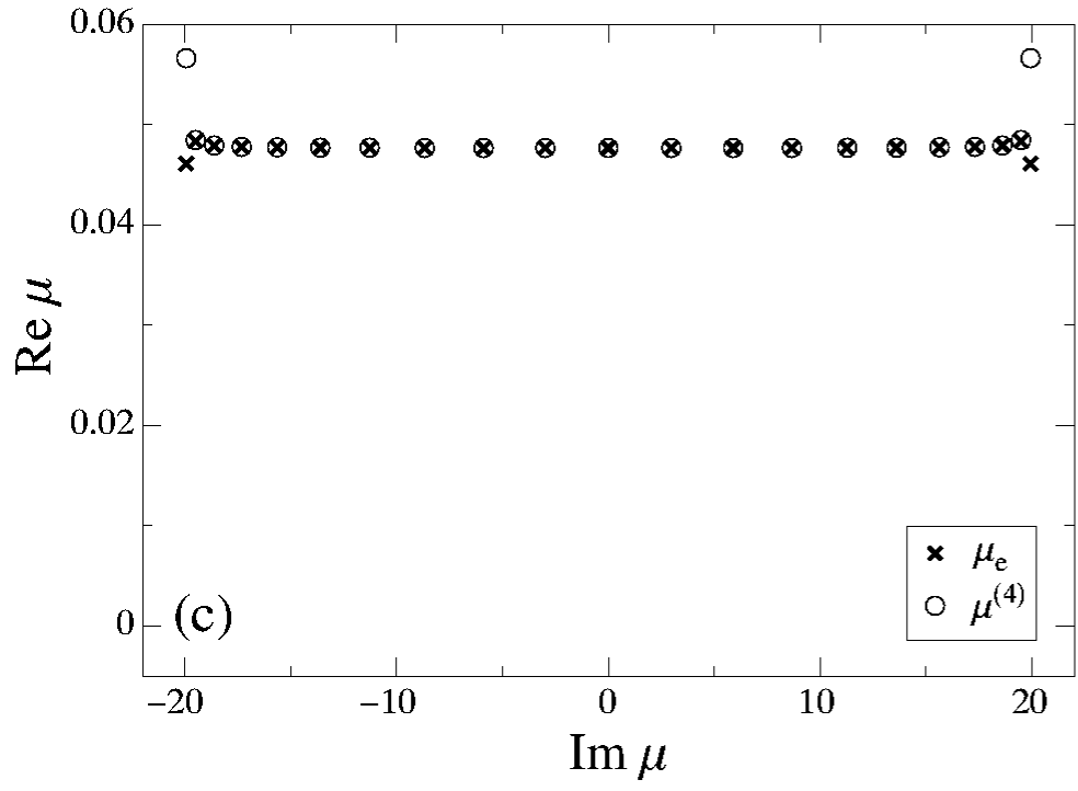
Figure 1: Eigenvalue spectrum for $N=21$ and given $q$: (a) $\beta=0.4$, (b) $\beta=0.7$, and (c) $\beta=10$. $\mu_{\rm e}$ denotes the exact eigenvalues obtained by numerical diagonalization and $\mu^{(i)}$ the eigenvalues of the different families given in Tables 1 and 2

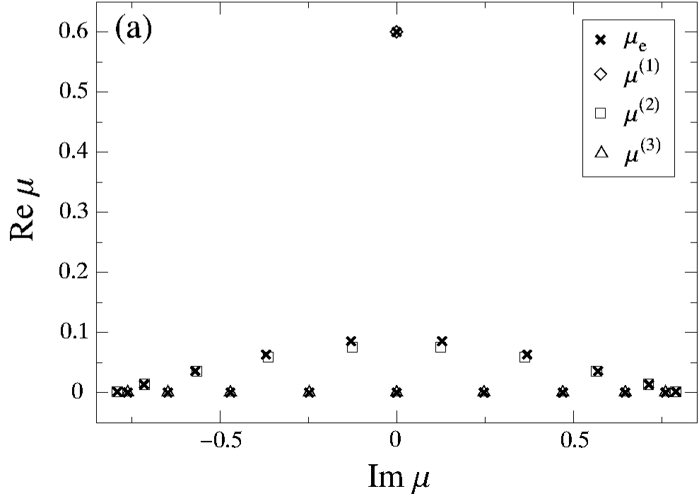
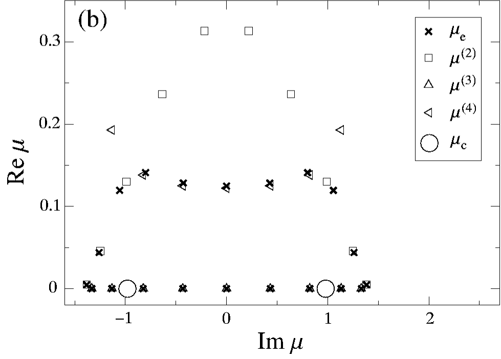
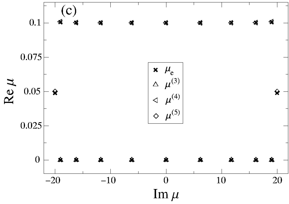
Figure 2: Eigenvalue spectrum for $N=20$ and $q$ even: (a) $\beta=0.4$, (b) $\beta=0.7$, and (c) $\beta=10$. $\mu_{\rm e}$ denotes the exact eigenvalues obtained by numerical diagonalization and $\mu^{(i)}$ the eigenvalues of the different families given in Tables 1 and 2

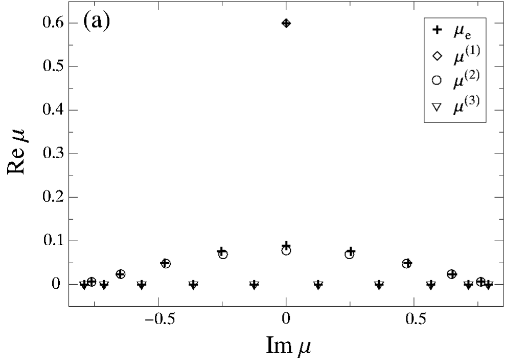
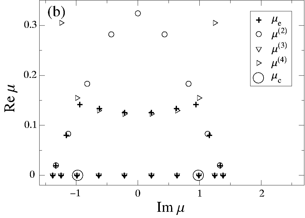
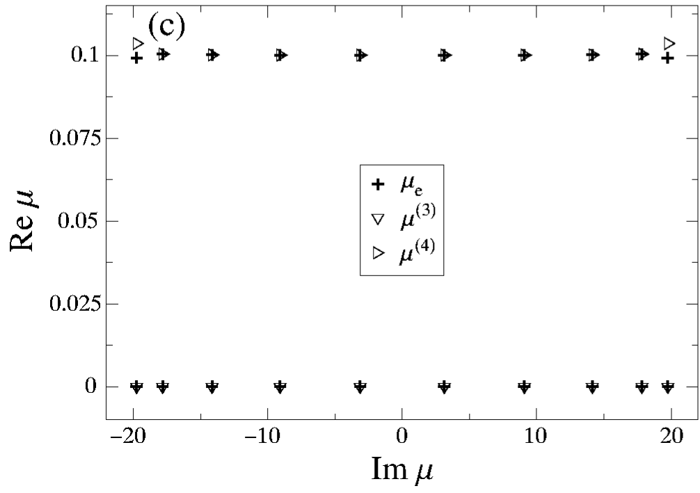
Figure 3: Eigenvalue spectrum for $N=20$ and $q$ odd: (a) $\beta=0.4$, (b) $\beta=0.7$, and (c) $\beta=10$. $\mu_{\rm e}$ denotes the exact eigenvalues obtained by numerical diagonalization and $\mu^{(i)}$ the eigenvalues of the different families given in Tables 1 and 2

For $\beta<\frac{1}{2}$, the analytical expressions of the eigenvalues which concern us are summarized in Table 1. Two families of eigenvalues ($\mu^{(1)}$ and $\mu^{(2)}$) enter in the discussion for $N$ odd, and three families ($\mu^{(1)}$, $\mu^{(2)}$, and $\mu^{(3)}$), for $N$ even. The numerical eigenvalues are plotted in Figs. 1(a), 2(a), and 3(a) and are in very good agreement with the analytical results. The sole diffusive eigenvalue $\mu^{(1)}$ has a real part and no imaginary part. The $N-1$ other eigenvalues, either belongs to the $\mu^{(2)}$ family for $N$ odd or to the $\mu^{(2)}$ and $\mu^{(3)}$ families for $N$ even. The eigenvalues $\mu^{(2)}$ and $\mu^{(3)}$ have an imaginary part which extends from $-2\beta$ to $2\beta$ and they generate oscillations in the dynamics. The real part of the $\mu^{(2)}$ eigenvalues is small and tends to zero in the large $N$ limit. The real part of the $\mu^{(3)}$ eigenvalues is always zero.

For $\beta>\frac{1}{2}$, the diffusive eigenvalue $\mu^{(1)}$ has disappeared after merging with the other eigenvalues and the situation is slightly more complicated. The situation for a moderate value of $\beta>\frac{1}{2}$ is depicted in Figs. 1(b), 2(b), and 3(b) while the analytical expressions of the eigenvalues are given in Table 2. Since $\mu^{(1)}$ no longer exists, we have the two families of eigenvalues $\mu^{(2)}$ and $\mu^{(4)}$ if $N$ is odd, and the three families $\mu^{(2)}$, $\mu^{(3)}$ and $\mu^{(4)}$ if $N$ is even. Two regions of the spectrum have to be distinguished. The eigenvalues $\mu^{(2)}$ exist in the region where $|\mu|>|\mu_{c}|$ while the eigenvalues $\mu^{(4)}$ exist in the region where $|\mu|<|\mu_{c}|$. We observe that the extra family of eigenvalues $\mu^{(4)}$ has appeared because of the collision with the diffusive eigenvalue $\mu^{(1)}$. We can see in Figs. 1(b), 2(b), and 3(b) that the analytical results of Table 2 reproduce very well the eigenvalues obtained by numerical diagonalization in the two regions. Here again, the number of eigenvalues is equal to $N$ for a given wavenumber $q$, the imaginary part of the eigenvalues extends from $-2\beta$ to $2\beta$, and the real parts of all eigenvalues tends to zero in the large $N$ limit.

A special situation occurs when $\beta>\frac{1}{2}$ is increased to large values. This situation is depicted in Figs. 1(c), 2(c), and 3(c). The situation is similar to the previous one but the region $|\mu|>|\mu_{c}|$ has disappeared so that the family of eigenvalues $\mu^{(2)}$ corresponding to the expansion $\beta\to 0$ no longer exists. For $N$ odd and for $N$ even with $q$ odd, these eigenvalues are replaced by the eigenvalues $\mu^{(4)}$ eigenvalues. For $N$ even and $q$ even, we find the two eigenvalues $\mu^{(5)}$ beside the family of eigenvalues $\mu^{(4)}$. The agreement between the analytical and numerical results is very good here also. As before, the imaginary part of all these eigenvalues extends from $-2i\beta$ to $2i\beta$ and their real parts tends to zero in the large $N$ limit.

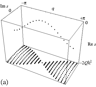
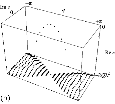
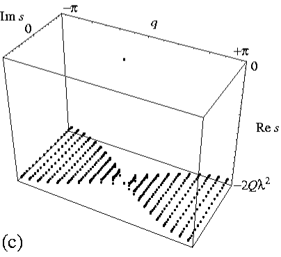
Figure 4: Complete spectrum of the eigenvalues $s_{q\theta}$ versus the wavenumber $q$ for the Redfield superoperator (II.2)-(25) The eigenvalues are given by Eq. (124) in terms of the eigenvalues $\mu_{q\theta}$ depicted in Figs. 1-3 at given values of the wavenumber. The size of the chain is here $N=21$. The parameter values are: (a) $\frac{A}{Q\lambda^{2}}=0.4$; (b) $\frac{A}{Q\lambda^{2}}=0.7$; (c) $\frac{A}{Q\lambda^{2}}=10$.

A global view of the complete spectrum of the $N^{2}$ eigenvalues of the Redfield superoperator is depicted in Fig. 4 by varying the wavenumber $q$ in a third dimension. Here, we only consider for simplicity the case where $N$ is odd. The relation between the wavenumber $q$ and the parameter $\beta$ is given by Eq. (48). The wavenumber $q$ varies in the first Brillouin zone or, equivalently, in the interval $0\leq q<2\pi$. We see in Fig. 4(a) that the diffusive eigenvalues $\mu^{(1)}$ exists for all the values of the wavenumber in the case $\frac{A}{Q\lambda^{2}}<\frac{1}{2}$ which implies $\beta<\frac{1}{2}$. However, if $\frac{A}{Q\lambda^{2}}>\frac{1}{2}$, the diffusive eigenvalue $\mu^{(1)}$ disappears as expected for some values of the wavenumber corresponding to $\beta>\frac{1}{2}$. This situation is observed in Fig. 4(b).

For very large values of $\frac{A}{Q\lambda^{2}}>\frac{1}{2}$, the diffusive branch of the spectrum is reduced to the sole eigenvalue at $q^{(1)}=0$, as seen in Fig. 4(c). In this case, diffusion has disappeared from the spectrum which only contains eigenvalues associated with damped oscillatory behavior. The diffusive branch can be supposed to have disappeared when its last nonzero eigenvalue disappears in Eq. (LABEL:spec3aae). Therefore the diffusive branch disappears when the value of $\beta$ for the first nonzero eigenvalue corresponding to $q=\frac{2\pi}{N}$ is larger than the critical value $\beta_{\rm c}=\frac{1}{2}$. This happens when the coupling parameter exceeds the critical value given by

$$\lambda_{\rm c}=\sqrt{\frac{2A}{Q}\sin\frac{\pi}{N}}\stackrel{{\scriptstyle N>5}}{{\simeq}}\sqrt{\frac{2A\pi}{QN}}\;.$$ (125)

This disappearance of the diffusion branch can be observed in Fig. 4(c). We notice that the diffusive branch always exists in the infinite-system limit ($N\to\infty$) in which case $\lambda_{\rm c}$ can be arbitrarily small.

We have described in this section the complete spectrum of the Redfield superoperator for a finite chain. We now briefly indicate which are the dynamical implications of these results.

IV.8 From the spectrum to the dynamics

The linear decomposition (26) of the density matrix shows that the modes which control the long-time dynamics correspond to the eigenvalues having the smallest absolute value of their real part. The eigenvalues with larger absolute value of their real part correspond to faster modes which control the relaxation on shorter time scales. For systems of finite size $N$, the long-time relaxation can be of two kinds. In the case where $\lambda<\lambda_{\rm c}$, the long-time relaxation is controlled by nondiffusive modes and consists in complicated oscillations of different periods damped at rates ${\rm Re}\,s\simeq-2Q\lambda^{2}$. This is due to the fact that, in this case, all the eigenvalues of the spectrum have a similar real part and different imaginary parts. This also indicates that the modes corresponding to the relaxation of the coherences (modes with complex eigenvalues) and of the populations (modes with real eigenvalues) decay on similar time scales. In the other case where $\lambda>\lambda_{\rm c}$, the long-time relaxation is controlled by the diffusive mode. This relaxation is free of any oscillations and is controlled by the rate $s\simeq-4\pi^{2}A^{2}/(Q\lambda^{2}N^{2})$. This diffusive relaxation exclusively concerns the populations of the system. The other nondiffusive modes describe the decoherence (as well as the relaxation of the populations beside the part controlled by diffusion when $2A>Q\lambda^{2}$). These modes decay at rates ${\rm Re}\,s\simeq-2Q\lambda^{2}$, i.e., on much shorter time scales than the diffusive mode. The dynamics of the finite $N$ system is studied in detail elsewhere Esposito .

V Infinite chain

The spectrum of the infinite chain coupled to its environment can be obtained from the spectrum of the finite chain in the infinite-size limit $N\to\infty$. The wavenumber $q$ becomes a continuous parameter varying in the first Brillouin zone $-\pi\leq q<\pi$.

For given wavenumber, the diffusive eigenvalue $\mu^{(1)}$ or $s^{(1)}$ given by Eq. (LABEL:spec3aae) remains isolated. Consequently, we obtain the result that the dispersion relation of diffusion is exactly given by the analytical expression

$$s_{q} = 2\sqrt{Q^{2}\lambda^{4}-\left(2A\sin\frac{q}{2}\right)^{2}}-2Q\lambda^{2}=-Dq^{2}+O(q^{4})\;.$$

The diffusion coefficient

$$D=\frac{A^{2}}{Q\lambda^{2}}\;,$$ (127)

is proportional to the square of the parameter $A$ of the tight-binding Hamiltonian and inversely proportional to the parameter $Q\lambda^{2}$ of the coupling to the environment. The transport is therefore due to the tunneling from site to site, which is hindered by the environmental fluctuations proportional to $Q\lambda^{2}$. It as been shown in Ref. Esposito that, for an Ohmic coupling to the environment, the diffusion coefficient is inversely proportional to the temperature. By using the Einstein relation between the diffusion coefficient and the conductivity, this latter is therefore inversely proportional to the square of the temperature.

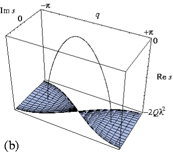
Figure 5: Spectrum of the infinite chain coupled to its environment: (a) in the regime $2A<Q\lambda^{2}$ for $A=0.4$ and $Q\lambda^{2}=1$; (b) in the regime $2A>Q\lambda^{2}$ for $A=0.6$ and $Q\lambda^{2}=1$ where the diffusive branch is limited to the wavenumbers $|q|<q_{\rm c}=1.97022$.

For $2A\leq Q\lambda^{2}$, the diffusive eigenvalue exists for all the values of the wavenumber $-\pi\leq q<+\pi$, as seen in Fig. 5(a).

For $2A>Q\lambda^{2}$, the diffusive eigenvalue only exists for all the values of the wavenumber in the range

$$-q_{\rm c}\leq q\leq+q_{\rm c}\;,\quad\mbox{with}\quad q_{\rm c}=2\arcsin\frac{Q\lambda^{2}}{2A}\;.$$ (128)

as seen in Fig. 5(b).

Beside the isolated diffusive eigenvalue, the spectrum at given wavenumber $q$ contains a continuous part obtained by the accumulation of the eigenvalues $\mu^{(2)}$, $\mu^{(3)}$, $\mu^{(4)}$, and $\mu^{(5)}$ in the limit $N\to\infty$. Indeed, in this limit, all these eigenvalues accumulate into a segment of straight line given by

$$s_{q\theta} = -4iA\left(\sin\frac{q}{2}\right)\;\cos\theta-2Q\lambda^{2}\;,$$ (129)

with $0\leq\theta\leq\pi$ and $-\pi\leq q<+\pi$ [see Eqs. (123) and (124)]. This part of the spectrum is also depicted in Fig. 5 and describes the time evolution of the quantum coherences which are damped at the exponential rate $-{\rm Re}\;s_{q\theta}=2Q\lambda^{2}$ with possible oscillations due to their nonvanishing imaginary part ${\rm Im}\;s_{q\theta}$.

The eigenvalue (LABEL:diff.infinite) can be considered as a Liouvillian resonance Pillet1 ; Pillet2 similar to the Pollicott-Ruelle resonances describing diffusion in classical systems Gasp96 ; Gasp98 .

VI Conclusions

In the present paper, we have studied an exactly solvable model of simple translationally invariant subsystems interacting with their environment. The coupling to the environment is described by correlation functions which are delta-correlated in space and time. The reduced dynamics of the subsystem is described by a Redfield quantum master equation which takes, for such environments, a Lindblad form. Thanks to the invariance under spatial translations, we can apply the Bloch theorem to the subsystem density matrix. In this way, we succeeded in getting analytical expressions for all the eigenvalues of the Redfield superoperator. These eigenvalues control the time evolution of the subsystem and its relaxation to the thermodynamic equilibrium. Two kinds of eigenvalues were obtained: the isolated eigenvalue (LABEL:diff.infinite) giving the dispersion relation of diffusion along the one-dimensional subsystem and the other eigenvalues (129) which describe the decay of the populations and quantum coherences. The process of decoherence in the subsystem is controlled by these latter eigenvalues (129).

The properties of the system depend on the length $N$ of the one-dimensional chain, on the width $4A$ of the energy band of the unperturbed tight-binding Hamiltonian and on the intensity $Q$ of the environmental noise multiplied in the combination $Q\lambda^{2}$ with the square of the coupling parameter $\lambda$ of perturbation theory.

We discovered that, for a finite chain, there are two regimes depending on the the chain length $N$ and the physical parameters $A$ and $Q\lambda^{2}$.

For a finite and small enough chain, there is a nondiffusive regime characterized by a time evolution with oscillations damped by decay rates proportional to $Q\lambda^{2}$. The oscillations are the time evolution of the quantum coherences. This nondiffusive regime exists if the coupling parameter is smaller than a critical value which is inversely proportional to the square root of the chain size $N$: $\lambda<\lambda_{\rm c}=O(N^{-\frac{1}{2}})$.

For larger chains, we are in the diffusive regime with a monotonic decay on long times at a rate controlled by the diffusion coefficient. In this regime, the slower relaxation mode relaxes exponentially in time with the scaling $t/(\lambda N)^{2}$.

In the limit of an infinite chain $N\to\infty$ and for non-vanishing coupling parameter $Q\lambda^{2}$, the nondiffusive regime disappears and the system always diffuses.

The diffusion coefficient is proportional to the square of the width $4A$ of the energy band and inversely proportional to the intensity $Q\lambda^{2}$ of the environmental noise. Accordingly, we are in the presence of a mechanism of diffusion in which the quantum tunneling of the particle from site to site is perturbed by the environmental fluctuations.

The eigenvalues of the Redfield superoperator obtained in the present paper give the Liouvillian resonances at the second order of perturbation theory. In this regard, the present work extends the results of Refs. Pillet1 ; Pillet2 on the spin-boson model to systems with a translational symmetry in space and capable of sustaining the transport property of diffusion beside simple decay processes. These Liouvillian resonances are the quantum analogues of the Pollicott-Ruelle resonances which have been studied elsewhere for diffusion in classical systems Gasp96 ; Gasp98 .

Table 1: For wavenumbers $q$ corresponding to $\beta<\frac{1}{2}$: List of the eigenvalues $\mu_{q\theta}$ of the matrix (58) given by Eq. (123). These eigenvalues are directly related to the Redfield superoperator eigenvalues by Eq. (124).

$N$ odd	$N=4I$ and $q$ even	$N=4I$ and $q$ odd
	or $N=4I+2$ and $q$ odd	or $N=4I+2$ and $q$ even
$\mu^{(1)}=\sqrt{1-(2\beta)^{2}}+2\frac{{\rm e}^{-2N{\rm arccosh}\;1/(2\beta)}}{\sqrt{1-(2\beta)^{2}}}$	$\mu^{(1)}=\sqrt{1-(2\beta)^{2}}+2\frac{{\rm e}^{-N{\rm arccosh}\;1/(2\beta)}}{\sqrt{1-(2\beta)^{2}}}$	$\mu^{(1)}=\sqrt{1-(2\beta)^{2}}-2\frac{{\rm e}^{-N{\rm arccosh}\;1/(2\beta)}}{\sqrt{1-(2\beta)^{2}}}$
$\mu^{(2)}\stackrel{{\scriptstyle\beta\to 0}}{{=}}-2i\beta\cos\frac{n\pi}{N}$	$\mu^{(2)}\stackrel{{\scriptstyle\beta\to 0}}{{=}}-2i\beta\cos\frac{(2n+1)\pi}{N}$	$\mu^{(2)}\stackrel{{\scriptstyle\beta\to 0}}{{=}}-2i\beta\cos\frac{2n\pi}{N}$
$\hskip 28.45274pt+\frac{4\beta^{2}}{N}\sin^{2}\frac{n\pi}{N}$	$\hskip 28.45274pt+\frac{8\beta^{2}}{N}\sin^{2}\frac{(2n+1)\pi}{N}$	$\hskip 28.45274pt+\frac{8\beta^{2}}{N}\sin^{2}\frac{2n\pi}{N}$
$\hskip 28.45274pt+\frac{16\beta^{4}}{3N}\sin^{4}\frac{n\pi}{N}$	$\hskip 28.45274pt+\frac{32\beta^{4}}{3N}\sin^{4}\frac{(2n+1)\pi}{N}$	$\hskip 28.45274pt+\frac{32\beta^{4}}{3N}\sin^{4}\frac{2n\pi}{N}$
$\hskip 28.45274pt+O(\frac{\beta^{6}}{N})+O(\frac{i\beta^{3}}{N^{2}})$	$\hskip 28.45274pt+O(\frac{\beta^{6}}{N})+O(\frac{i\beta^{3}}{N^{2}})$	$\hskip 28.45274pt+O(\frac{\beta^{6}}{N})+O(\frac{i\beta^{3}}{N^{2}})$
for $n=1,2,\ldots,N-1$	for $n=0,1,\ldots,\frac{N}{2}-1$	for $n=1,2,\ldots,\frac{N}{2}-1$
	$\mu^{(3)}=-2i\beta\cos(\frac{2n\pi}{N})$	$\mu^{(3)}=-2i\beta\cos(\frac{(2n+1)\pi}{N})$
	for $n=1,2,\ldots,\frac{N}{2}-1$	for $n=0,1,\ldots,\frac{N}{2}-1$

Table 2: For wavenumbers $q$ corresponding to $\beta>\frac{1}{2}$: List of the eigenvalues $\mu_{q\theta}$ of the matrix (58) given by Eq. (123). These eigenvalues are directly related to the Redfield superoperator eigenvalues by Eq. (124).

$N$ odd	$N=4I$ and $q$ even	$N=4I$ and $q$ odd
	or $N=4I+2$ and $q$ odd	or $N=4I+2$ and $q$ even
If $|\mu^{(4)}|<|\mu_{c}|$:
$\mu^{(4)}\stackrel{{\scriptstyle\beta\to\infty}}{{=}}-2i\beta\cos\frac{(n+\frac{1}{2})\pi}{N}$	$\mu^{(4)}\stackrel{{\scriptstyle\beta\to\infty}}{{=}}-2i\beta\cos\frac{2n\pi}{N}$	$\mu^{(4)}\stackrel{{\scriptstyle\beta\to\infty}}{{=}}-2i\beta\cos\frac{(2n+1)\pi}{N}$
$\hskip 28.45274pt+\frac{1}{N}(1+\frac{1}{12\beta^{2}\sin^{2}\frac{(n+(1/2))\pi}{N}}$	$\hskip 28.45274pt+\frac{2}{N}(1+\frac{1}{12\beta^{2}\sin^{2}\frac{2n\pi}{N}}$	$\hskip 28.45274pt+\frac{2}{N}(1+\frac{1}{12\beta^{2}\sin^{2}\frac{(2n+1)\pi}{N}}$
$\hskip 56.9055pt+\frac{1}{32\beta^{4}\sin^{4}\frac{(n+(1/2))\pi}{N}})$	$\hskip 56.9055pt+\frac{1}{32\beta^{4}\sin^{4}\frac{2n\pi}{N}})$	$\hskip 56.9055pt+\frac{1}{32\beta^{4}\sin^{4}\frac{(2n+1)\pi}{N}})$
$\hskip 28.45274pt+O(\frac{1}{\beta^{6}N})+O(\frac{i}{\beta N^{2}})$	$\hskip 28.45274pt+O(\frac{1}{\beta^{6}N})+O(\frac{i}{\beta N^{2}})$	$\hskip 28.45274pt+O(\frac{1}{\beta^{6}N})+O(\frac{i}{\beta N^{2}})$
for $n_{\rm min}<n<n_{\rm max}$	for $n_{\rm min}<n<n_{\rm max}$	for $n_{\rm min}<n<n_{\rm max}$
	$\mu^{(5)}\stackrel{{\scriptstyle\beta\to\infty}}{{=}}\mp 2i\beta+\frac{1}{N}+O(\frac{1}{\beta})$
If $|\mu^{(2)}|>|\mu_{c}|$:
$\mu^{(2)}\stackrel{{\scriptstyle\beta\to 0}}{{=}}-2i\beta\cos\frac{n\pi}{N}$	$\mu^{(2)}\stackrel{{\scriptstyle\beta\to 0}}{{=}}-2i\beta\cos\frac{(2n+1)\pi}{N}$	$\mu^{(2)}\stackrel{{\scriptstyle\beta\to 0}}{{=}}-2i\beta\cos\frac{2n\pi}{N}$
$\hskip 28.45274pt+\frac{4\beta^{2}}{N}\sin^{2}\frac{n\pi}{N}$	$\hskip 28.45274pt+\frac{8\beta^{2}}{N}\sin^{2}\frac{(2n+1)\pi}{N}$	$\hskip 28.45274pt+\frac{8\beta^{2}}{N}\sin^{2}\frac{2n\pi}{N}$
$\hskip 28.45274pt+\frac{16\beta^{4}}{3N}\sin^{4}\frac{n\pi}{N}$	$\hskip 28.45274pt+\frac{32\beta^{4}}{3N}\sin^{4}\frac{(2n+1)\pi}{N}$	$\hskip 28.45274pt+\frac{32\beta^{4}}{3N}\sin^{4}\frac{2n\pi}{N}$
$\hskip 28.45274pt+O(\frac{\beta^{6}}{N})+O(\frac{i\beta^{3}}{N^{2}})$	$\hskip 28.45274pt+O(\frac{\beta^{6}}{N})+O(\frac{i\beta^{3}}{N^{2}})$	$\hskip 28.45274pt+O(\frac{\beta^{6}}{N})+O(\frac{i\beta^{3}}{N^{2}})$
for $n=1,2,\ldots,n_{\rm min}$	for $n=0,1,\ldots,n_{\rm min}$	for $n=1,2,\ldots,n_{\rm min}$
and $n=n_{\rm max},...,N-1$	and $n=n_{\rm max},...,\frac{N}{2}-1$	and $n=n_{\rm max},...,\frac{N}{2}-1$
	$\mu^{(3)}=-2i\beta\cos(\frac{2n\pi}{N})$	$\mu^{(3)}=-2i\beta\cos(\frac{(2n+1)\pi}{N})$
	for $n=1,2,\ldots,\frac{N}{2}-1$	for $n=0,1,\ldots,\frac{N}{2}-1$

.

.

.

.