Self-propelled non-linearly diffusing particles. Aggregation and continuum description.

Abstract

We introduce a model of self-propelled particles carrying out a Brownian motion with a diffusion coefficient which depends on the local density of particles within a certain finite radius. Numerical simulations show that in a range of parameters the long-time spatial distribution of particles is non-homogeneous, and clusters can be observed. A number density equation, which explains the emergence of the aggregates and indicates the values of the parameters for which they appear, is derived. Numerical results of this continuum density equation are also shown.

The tendency of living individuals to aggregate is an ubiquitous phenomenon in Nature that constitutes a central problem in different areas of the natural sciences. The usually discussed examples in the literature arise from very diverse contexts and comprise a wide range of spatiotemporal scales: human crowds, animal groups, cell populations or bacteria colonies. In this context distinct situations are studied, including the dynamics of groups of individuals moving coherently resembling the behavior of fish schools, bird flocks or insect swarms flierl , the pattern formation in populations of bacteria murray , or the patchy structure of plankton mediated by hydrodynamic driving nuestroreview . Two levels of descriptions are usually performed, one considering the discrete particle dynamics, and the other accounting for the large spatiotemporal scales in terms of an evolution equation for the number density of particles. In the best of the cases, the last is derived from the more fundamental particle dynamics.

From the theoretical point of view one of the main questions one can address is about what causes aggregation to form keshet . In order to answer this, and starting from the discrete particle dynamics, many different mathematical models have been introduced which, mainly in the physics literature, are characterised by their simplicity but also because they retain the basic features underlying the clustering phenomenon. Essentially these models assume that i) individuals are self-propelled, and ii) they interact with the environment and/or with other particles through attractive and repulsive forces flierl , or rather, by modifying its velocity because of communications with neighbours VM . Note, however, that even a simpler mechanism that cannot be classified within ii) and that gives rise to clustering has been introduced in young .

In this letter, following this line of searching simplicity, we introduce a basic model going through steps i) and ii) characterised because the aggregation phenomenon is due to a new type of mechanism, where no attractive nor repulsive forces among particles are taken into account. The model considers a fix population of particles moving Brownianly. At every time step, any particle modifies, reducing, its random motility (diffusion coefficient) depending on the total number of particles in a neighbourhood of spatial range $R$. This response of the particles to their local environment can be interpreted as an effective deceleration because of the presence (via collisions, interchange of chemicals, excluded volume effects, demographic pressure, etc…) of other particles. The interaction radius $R$ appears frequently in the modelling of biological systems to take into account visual or hearing stimuli, chemical signaling, and other kinds of interactions at a distance. $R$ is considered to be a fixed number in this work but in some biological species it depends on the environmental conditions. Just as an example, we mention the detection distance of preys for a type of zooplankton jpr . In our model, despite the particles are moving randomly and no attractive forces among them are considered, they tend to cluster. It will be obvious, when the coarse-grained number density equation of the model is presented, that this is because of the nonlinear character of the diffusion of the particles. Therefore, the aim of this work is to introduce this new type of mechanism, the local modification of the motility by the crowding of the surroundings, at the level of discrete particle dynamics, and show under which conditions it gives rise to clustering. Then obtain its continuum description and interpret the model and its clustering instability in terms of this. The manuscript goes precisely along these lines: first we introduce the particle model and study it numerically, then we derive its continuum description and study it analytically and numerically.

Let us consider $N$ pointwise particles initially distributed randomly in a two-dimensional system of size $L\times L$ with periodic boundary conditions. At every discrete time step $t$ the positions of all the particles, ${\bf x}_{i}(t)=(x_{i}(t),y_{i}(t))$ ($i=1,...,N$), are updated synchronously as follows:

$$x_{i}(t+\Delta t)=x_{i}(t)+\sqrt{\frac{2D_{0}\Delta t}{(N_{R}(i))^{p}}}\eta^{x}_{i}(t),$$

$$y_{i}(t+\Delta t)=y_{i}(t)+\sqrt{\frac{2D_{0}\Delta t}{(N_{R}(i))^{p}}}\eta^{y}_{i}(t),$$ (1)

where $D_{0}$ is a constant named in the following constant diffusivity or motility (this last name is the usual one for cells, bacteria or plankton organisms), $\Delta t$ is the time step which we take equals to $1$ in the numerical simulations, $\mbox{\boldmath$\eta$}=(\eta^{x},\eta^{y})$ is a white noise with zero mean and correlations $<\eta^{a}_{i}(t),\eta^{b}_{j}(t^{\prime})>=\delta_{ab}\delta_{ij}\delta_{tt^{\prime}}$. $N_{R}(i)$ denotes the total number of particles at distance less than $R$ of particle $i$ including itself, and $p$ is a positive real number. The model clearly states that particles are moving Brownianly with diffusion coefficient inversely proportional to the number of neighbours within a range $R$, $D_{i}=D_{0}/(N_{R}(i))^{p}$, being $D_{i}$ the effective diffusivity of particle $i$. In this way, if the neighbourhood of a particle is poorly crowded it diffuses quickly. The functional dependence of $D_{i}$ resembles the standard models of density-dependent dispersal of insects or animals murray , where the behavioral parameter $p$ determines this dependence. Note, however, that in in these models, at difference with the one introduced in this work, the diffusivity increases with the density of particles. A distinct type of decreasing function of $D_{i}$ with $N_{R}(i)$ could be considered, and will be discussed later on at the level of the density equation.

First, we pay attention to the limits $R\to 0$ and $R\to L$ (because of periodic boundary conditions the total system size limit for $R$ is in fact smaller than $L$ but we keep this notation just for clarity). In the first one, $N_{R}(i)=1$ for all $i$ so that the particles diffuse with the constant motility, $D_{i}=D_{0}$. In the second limit again all the particles diffuse with the same diffusion coefficient given by $D_{i}=D_{0}/N$, that is negligible for large $N$. Of course we do not expect any grouping behavior in these two limits and $R$ will be considered in the rest of the paper to be in the interval $0<R<L$. In addition, for large values of $p$ the diffusivity of the particles is almost zero, so we neither consider them. Similarly, very small values of $D_{0}$ are disregarded.

Numerical simulations of eq. (1) show that a statistical steady state of the particles distribution is reached. We observe this by computing the cluster coefficient of the distribution of particles (see below), and observing that for long-times it goes to an average constant value, which indicates that the spatial distribution of particles is statistically stationary (see fig. (1)). For the statistical stationary state we also note that: a) for a wide range of values of $D_{0}$ and $R$ the long-time spatial distribution of particles is homogeneous if $p$ is in the range $0<p\leq 1$; b) for $p>1$ the particles distribute non-uniformly for all the values of $D_{0}$ and $R$ considered. Increasing the value of $p$ upon the critical value $p_{c}=1$ the unhomogeneous distribution of particles turns into clusters. However, if we keep on increasing $p$ (as already suggested in the former paragraph) the effective diffusivity, $D_{i}$, is almost zero and the particles remain almost without moving, so that the time scales to observe a nonhomogenous distribution become very large. The aggregation proceeds as follows: if a number particles are close to each other their effective diffusivity diminishes and they do not get much appart forming a small cluster. As other particles, which are moving randomly in the system, get near this cluster, their diffusivity is reduced and they stay in the aggregate.

No cluster dynamics is observed in the system. The groups of particles remain statistically fixed in the space, not changing notably their position, since most of the particles in any of them have a very small diffusivity. Only the particles in the outer parts have a non-negligible diffusion coeficient and slightly move, never getting far of the cluster and only very rarely leaving the cluster and joining to another one. In principle, it could be surprising that large values of $D_{0}$ do not avoid any possibility of aggregation in the system. In fact, in the numerical simulations one observes that larger values of $D_{0}$ favour encounters among particles and the clustered steady state is reached in a shorter time. Thus, the value of $D_{0}$ in the model only changes the time scale of the system. As already mentioned, increasing values of $p$ homogenises the spatial distribution of particles, i.e. they are more sparsed in the system, and the number of groups increases. When clusters are formed in the system, their typical size strongly depends on the values of the parameters $R$, $p$ and the initial number of particles. Also, it is always observed that the clusters do not periodically distribute in space nostropre which is what is expected for realistics models of swarming since periodicity is rarely seen in these mogilnerkeshet . In fig. (2) we show distinct spatial structures observed for different values of the parameters. A single cluster and several clusters are shown there.

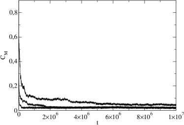
Figure 1: We see in this figure the approach to the steady state. We plot the clustering coefficient, which gives an idea of the spatial distribution of particles (see text), vs time for different values of $D_{0}$ and the same value of $p=2$. From top to bottom: $D_{0}=10^{-5}$, $D_{0}=10^{-4}$, $D_{0}=10^{-3}$. The smaller $D_{0}$ the larger the time needed to reach the steady state.

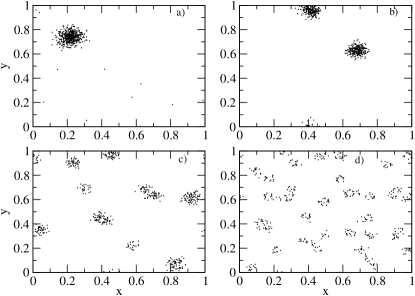
Figure 2: Long-time ($10^{7}$ time steps) spatial distribution of particles. The parameters are $R=0.05$, initial density $\rho_{0}=500$ for all the plots, and a) $D_{0}=10^{-4}$, $p=1.5$; b) $D_{0}=10^{-5}$, $p=2.0$; c) $D_{0}=10^{-5}$, $p=3.5$; d) $D_{0}=10^{-3}$, $p=7.5$. The system size is $L=1$.

Clustering is quantified by using an entropy-like measure $S_{M}=-\sum_{i=1}^{M}\frac{m_{i}}{N}\ln\frac{m_{i}}{N}$, where $M$ is the number of boxes in which we divide the system, and $m_{i}$ is the number of particles inside box $i$. One has that $0\leq S_{M}\leq\ln M$, so that the minimum value, $S_{M}=0$, is obtained when all the particles are in just one of the boxes, and the maximum one, $\ln M$, is reached when $m_{i}=N/M$ for all $i$, i.e., $S_{M}$ decreases when there is more aggregation. The clustering coefficient is defined as $C_{M}=\exp(<S_{M}>_{t})/M$, where $<.>_{t}$ denotes a temporal average in steady state conditions, so that when there is no clustering $C_{M}\approx 1$ and small values of $C_{M}$ indicate a non-uniform distribution of particles. In fig. (3) we plot $C_{M}$ versus $p$ for different values of $D_{0}$, and always a fixed $R=0.05$ (similar plots, not shown, are obtained for other $R$’s). The transition at $p_{c}=1$ is clearly observed for the different values of $D_{0}$. In addition, for a fixed $D_{0}$ one can also see that as $p$ increases (for values in the clustering phase, $p>p_{c}$) $C_{M}$ also increases. This indicates that the number of clusters in the system gets larger as $p$ increases, as can be observed in fig. 2b) and c).

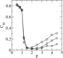
Figure 3: Clustering coefficient versus the parameter $p$. Each plot corresponds to a fixed value of $D_{0}$. The circles correspond to $D_{0}=10^{-5}$, squares to $D_{0}=10^{-4}$, and diamonds to $D_{0}=10^{-3}$. The rest of the parameters are $R=0.05$ and $\rho_{0}=500$. The system is divided in a number of $M=144$ boxes and every point in this figure is calculated from a spatial distribution of particles at time $t=10^{7}$.

In order to obtain a continuum description of the model to try to understand better its properties, we first take the limit $\Delta t\to 0$ in eq. (1) and get the Langevin equation

$$d{\bf x}_{i}(t)=\beta({\bf x}_{i}(t),t)d{\bf W}_{i}(t),\ \ i=1,...,N,$$ (2)

where $d{\bf W}_{i}(t)$ is a Wiener proccess and $\beta({\bf x}_{i}(t),t)=\sqrt{2D_{0}/N_{R}(i)^{p}}$. It is very important to note that eq. (2) should be interpreted in the Ito Calculus. This is so because it represents the continuous time limit of a discrete population dynamics model of nonoverlapping generations. A clear discussion on this can be consulted in the first of the references in vankampen .

Then the mean-field number density equation for eq. (2) (particularly appropriate for not too small densities) is given by vankampen

$$\frac{\partial\rho({\bf x},t)}{\partial t}=\frac{1}{2}\nabla^{2}(\beta({\bf x},t)^{2}\rho({\bf x},t)),$$ (3)

where $\rho({\bf x},t)$ is the number density of particles in the continuum space-time. Taking into account that in the continuum limit $N_{R}(i)=N_{R}({\bf x})=\int_{|{\bf x}-{\bf r}|\leq R}d{\bf r}\rho({\bf r},t)$, the final evolution equation for the density in our model is

$$\frac{\partial\rho({\bf x},t)}{\partial t}=D_{0}\nabla^{2}\left(\frac{\rho({\bf x},t)}{\left(\int_{|{\bf x}-{\bf r}|\leq R}d{\bf r}\rho({\bf r},t)\right)^{p}}\right),$$ (4)

with initial condition $\rho({\bf x},0)=N/L^{2}$. A proper derivation of eq. (4) from the interacting particle dynamics, eq. (2), gives rise to a multiplicative noise term that has been averaged out in eq. (4). As already mentioned, this is a good approximation for not too small densities. Moreover, fluctuations in the density equation, which reflect the discrete nature of the particles, seem to have an irrelevant role in the pattern formation instability to be discussed below (see also nostropre ).

Particle number is conserved in eq. (4) and also it is implicitly assumed that when the density at a point is zero within a range $R$ it remains zero (any possible singularity is avoided in eq. (4)). In this density equation it is clear that the system is described by a nonlinear diffusion equation where the effective diffusivity at any point is decreased by the total density in a neighbourhood of the point. With respect to other existent nonlinear diffusion models, e.g. for insect swarming murray , our model presents the following crucial differences: the finite range of interaction $R$, and that, as has already been mentioned, in those classical models the motility is generally proportional to the local density, at least to the author best knowledge. The following non-dimensionalization $s=D_{0}t/R^{2}$, ${\bf u}={\bf x}/R$ and $\bar{\rho}=R^{2}\rho$ transforms eq.(4) into

$$\frac{\partial\bar{\rho}({\bf u},s)}{\partial s}=\nabla_{\bf u}^{2}\left(\frac{\bar{\rho}({\bf u},s)}{\left(\int_{|{\bf u}-{\bf v}|\leq 1}d{\bf v}\bar{\rho}({\bf v},t)\right)^{p}}\right),$$ (5)

from which it is clear that $D_{0}$ only renormalizes the time-scale of the system.

To study the clustering, let us make a linear stability analysis of the stationary homogeneous solution, $\rho_{0}=N/L^{2}$, of eq. (4) . We write $\rho({\bf x},t)=\rho_{0}+\epsilon\psi({\bf x},t)$ where $\epsilon$ is a small parameter, and $\psi({\bf x},t)$ the space-time dependent perturbation, and substitute it in eq. (4). To first order in $\epsilon$, $\psi$ evolves as stratonovich :

$$\partial_{t}\psi({\bf x},t)=\frac{D_{0}}{(\rho_{0}\pi R^{2})^{p}}\nabla^{2}\psi-$$

$$\frac{D_{0}p}{\rho_{0}^{p}(\pi R^{2})^{p+1}}\nabla^{2}\left(\int_{|{\bf x}-{\bf r}|\leq R}\psi({\bf r},t)\,d{\bf r}\right).$$ (6)

Then taking an harmonic perturbation $\psi({\bf x},t)=\exp(\lambda t+i{\bf k}\cdot{\bf x})$ one arrives at the following dispersion relation

$$\lambda(K)=\frac{D_{0}K^{2}}{(\rho_{0}\pi R^{2})^{p}}(\frac{2pJ_{1}(KR)}{KR}-1),$$ (7)

being $K$ the modulus of ${\bf k}$, and $J_{1}$ the first-order Bessel function. (Non-dimensionalising eq. (7), or rather performing the stability analysis directly to the non-dimensional expression eq. (5), one has that $\bar{\lambda}(\bar{K})=(\bar{K}^{2}/(\bar{\rho}_{0}\pi)^{p})(\frac{2pJ_{1}(\bar{K})}{\bar{K}}-1)$, where $\bar{K}=KR$ and $\bar{\lambda}=\lambda R^{2}/D_{0}$.) The uniform density is unstable, giving rise to aggregation, if $\lambda$ is positive. For $K=0$ one has that $\lambda=0$ for all $p$ (and any $D_{0}$, $\rho_{0}$ and $R$). This implies that the homogeneous density is neutrally stable to uniform perturbations which is due to the conservation of the total number of particles. As shown in fig. (4) the growth rate $\lambda$ (always a real number) is positive for $p>1$, while the system is stable for $p\leq 1$. This is in agreement with the numerical results found for the discrete model. Moreover, the instability for values of $p$ larger than $1$ is in a band of wave vectors within the range $0\leq K\leq K_{+}$, i.e., it is of type II in the classification of crosshohenberg . This kind of instability appears typically for systems with a conservation law, and are characterised by the fact that the growth rate, $\lambda$, vanishes at K=0, and represents the onset of aggregation and formation of groups mogilnerkeshet . The phenomenology of aggregation already observed in the particle model has its perfect counterpart in the dispersion relation eq. (7), being the values of $D_{0}$, $\rho_{0}$ and $R$ irrelevant for the onset of clustering. Therefore, the density equation perfectly explains the aggregation of the particles as a deterministic instability of type II. The nonlinearities of the model saturate the exponential linear growth for $p>1$ given by the dispersion relation. It is worth mentioning that if an exponentially decreasing dependence fo the diffusivity would have been considered, $D(i)\propto\exp{-(pN_{R}(i))}$, a similar relation dispersion is obtained but with a control parameter $\tilde{p}$ dependent on $R$ and $\rho_{0}$, which is also rather realistic.

Figure 4: Dispersion relation, eq. (7), for different values of $p$. In the vertical we plot the (non-dimensional) growth exponent $\bar{\lambda}$ multiplied by $(\bar{\rho}_{0}\pi)^{p}$, and in the horizontal axis $\bar{K}=KR$. $p=1$ is the critical value for the instability.

We have also performed a numerical simulation of the density equation eq. (4) starting from a random initial distribution and using a variable time step in order to avoid any numerical instability. A long-time non-uniform non-periodic pattern is plotted in fig. (5) for $D_{0}=10^{-3}$, $R=0.1$, $\rho_{0}=76.23$ and $p=2$. As expected, but not shown, if $p\leq 1$ a uniform distribution of the field is obtained for these and other parameter values.

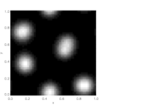
Figure 5: Density distribution at large time. $D_{0}=10^{-3}$, $R=0.1$, $\rho_{0}=76.23$ and $p=2$. Lighter colour indicates larger density.

In summary, a new mechanism for clustering of self-propelled particles has been presented. It just considers that the motility of any particle decreases with the crowding of its surroundings. The model has been studied and its number density equation has been obtained, which turns out to be a particular form of a nonlinear diffusion equation. The relation dispersion indicating the conditions for clustering were calculated, so that the clustering at the particle level can be understood as a deterministic instability of the density equation. In addition, the role of the parameters of the model becomes clearer at the density description level. Regarding a biological application, motile bacteria or plankton particles propel themself, so that they are typically modelled as self-propelled particles, and maybe a minimal mechanism like the one discussed in this work can explain some of the yet unknown causes for their clustering. Ongoing research on the nature of the transition to clustering VM ; chate , on other possible functional shapes of the motility of the particles, and on the influence of a variable interaction range are in consideration for the next future.

I acknowledge a very useful conversation with Emilio Hernández-García and also a critical reading of the manuscript. Financial support from MEC (Spain) and FEDER through project CONOCE2 (FIS2004-00953) is greatly acknowledged. C.L. is a Ramón y Cajal fellow of the Spanish MEC.

References

- (1) G. Flierl, D. Grunbaum, s. Levin, and D. Olson, J. Theor. Biol. 196, 397 (1999).
- (2) J.D. Murray, Mathematical biology, Springer-Verlag, Berlin (2002).
- (3) See for example E. Hernández-García, C. López, Z. Neufeld, Proceedings of the 2001 ISSAOS School on Chaos in Geophysical Flows, Ed. by G. Boffetta, G. Lacorata, G. Visconti, and A. Vulpiani, Otto Editore (Torino, 2004) (also in nlin.CD/0205009), and references therein.
- (4) L. Edelstein-Keshet, Mathematical models of swarming and social aggregation, in The 2001 International Symposium on Nonlinear Theory and its Applications, Miyagi, Japan (2001).
- (5) T. Vicsek et al., Phys. Rev. Lett. 75, 1226 (1995).
- (6) W.R. Young, A.J. Roberts, G. Stuhne, Nature 412, 328 (2001).
- (7) A.W. Visser and U.H. Thygesen, J. Plankton Res. 25, 1157 (2003).
- (8) A system where periodically arranged clusters are formed is introduced in E. Hernández-García and C. López, Phys. Rev. E 70, 016216 (2004).
- (9) A. Mogilner and L. Edelstein-Keshet, J. Math. Biol, 38, 534 (1999).
- (10) W. Horsthemke and R. Lefever, Noise-induced transitions, (Springer, Berlin, 1984); N.G. van Kampen, Stochastic processes in physics and chemistry, 2nd ed. (North-Holland, Amsterdam, 1992); C.W. Gardiner, Handbook of Stochastic Methods, 2nd ed. (Springer, Berlin, 1985).
- (11) If we would have taken, wrongly, Eq. (4) in its Stratonovich sense, the evolution equation for the perturbation is given by just the diffusion term. No instability is then observed in this wrong framework.
- (12) M. Cross and P. Hohenberg, Rev. Mod. Phys. 65, 851 (1993).
- (13) G. Grégoire and H. Chaté, Phys. Rev. Lett. 92, 025702 (2004).