A hard-sphere model on generalised Bethe lattices: Dynamics

Abstract

We analyse the dynamics of a hard-sphere lattice gas on generalised Bethe lattices using a projective approximation scheme (PAS). The latter consists in mapping the system’s dynamics to a finite set of global observables, closure of the resulting equations is obtained by approximating the true non-equilibrium state by a pseudo-equilibrium based only on the value of the observables under consideration. We study the liquid–crystal as well as the liquid–spin-glass transitions, special attention is given to the prediction of equilibration times and their divergence close to the phase transitions. Analytical results are corroborated by Monte-Carlo simulations.

I Introduction

The statistical mechanics of finite-connectivity systems has seen a large increase in interest within the last decade. The major reason for this interest was the emergence of a close interdisciplinary collaboration between statistical mechanics and theoretical computer science. In many hard combinatorial problems, phase transitions in resolvability and algorithmic performance were observed – once these problems are suitably randomised ChKaTa ; MiSeLe ; KiSe . This observation obviously provides a large temptation to use statistical mechanics tools to get insight into the problem structure going beyond the one which can be obtained with traditional tools from discrete mathematics and computer science. The natural mapping of these models to disordered finite-connectivity models was therefore used to investigate problems like satisfiability MoZe ; nature ; science , vertex cover vc_prl , graph colouring col_prl etc.

Coming back to physical models, finite-connectivity systems can be understood as an intermediate step between fully-connected mean-field models MePaVi and realistic, finite-dimensional systems. Even if their structure is not geometrical in the sense that they are embeddable into any finite-dimensional space, the finite connectivity allows for a reasonable implementation of notations like neighbourhood, distance etc. This property enables construction and analysis of microscopically motivated models, in particular for spin-glasses MePa ; MePa2 and structural glasses FrMeRiWeZe ; BiMe ; weigt ; PiTaCaCo ; rivoire ; HaWe .

The understanding of these models is, however, mainly based on the analysis of their thermodynamic equilibrium behaviour. Due to a technical break-through based on an application of the cavity method to finite-connectivity models MePa , the structure of stable and metastable states, the appearance of phase transitions etc. are relatively well-understood by now.

The knowledge is much less evolved in what concerns the dynamics of finite-connectivity models BaZe ; MoRi ; CuSe ; SeCuMo ; SeWe ; coolen1 . Here we will use an approximation scheme first introduced to analyse the dynamical behaviour of stochastic local-search algorithms for combinatorial optimisation SeMo ; BaHaWe . We will, however, use a different formulation which is based on the observation from Ref. SeWe that the method can be put into the canonical form of a projective approximations scheme being equivalent to the dynamical replica theory CoSh ; CoSh2 ; LaCoSh which was originally developed for fully connected systems. Note also coolen2 , where the same method was recently applied to Ising models on random graphs.

The model studied here is a hard-sphere lattice-gas model on a generalised Bethe lattice, which was first proposed in weigt as a microscopically motivated, but solvable model for the structural glass transition. The equilibrium behaviour of this model, including crystallisation as well as glass formation, was studied in great detail in HaWe . The present work, which is concentrated on the relaxational dynamics of the model, can be seen as a natural continuation of the work presented therein. Even if we have tried to make the present paper as self-contained as possible, sometimes we have to refer to technical details in the previous publication – whose full inclusion would go beyond the scope of the present article.

The paper is organised as follows. Sec. II gives an introduction to the system including a brief review of its static properties and the definition of the dynamics. In the following section, the general outline of the applied approximation scheme is presented. Sec. IV is dedicated to crystallisation dynamics, containing two approximations and comparison with Monte-Carlo simulations. In Sec. V an approximation of the dynamics near the spin-glass transition is presented. Finally, conclusion and outlook are given in the last section.

II The model

In a first step, we are going to define the model itself, review its static properties which were analysed in detail in HaWe . In the second part of this section we will define microscopic physical dynamics for the model, whose analysis will be the subject of the whole paper.

II.1 Construction and static properties

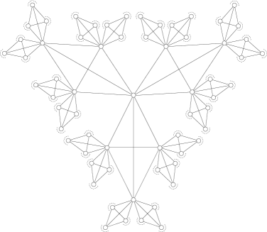
Figure 1: Part of a generalised Bethe-lattice with $k=2$, $p=3$. The 21 cliques connecting the central vertex to its nearest and second neighbours are shown. Figure from Ref. HaWe .

The system is a lattice gas of hard spheres living on a generalised Bethe lattice. Let us first specify the character of the particles. The property of hard spheres is realised by introducing an excluded volume associated with each particle. This is done by requiring that two neighbouring sites (i.e. sites that are connected with an edge in the graph) cannot be occupied simultaneously. Two particles have thus a minimal distance of two on the lattice.

The generalised Bethe lattice is constructed in the following way: The basic building blocks are small completely connected sub-graphs (i.e. cliques), each of which contains $p+1$ vertices. In each vertex $k+1$ of these cliques are merged. This procedure leads to a graph which is locally isomorphic to that shown in Fig. 1 for one specific choice of $k$ and $p$. The ideal graph can be thought of as an infinite continuation of the shown structure such that the whole graph remains loop-less apart from the inner-clique loops. Note that the ordinary Bethe lattice can be obtained as the special case $p=1$. It is furtheron obvious that a close packing on such a lattice consists of a configuration where each clique carries exactly one particle – which, because of the hard-sphere constraint, realises also the maximum particle density that can be found in a single clique.

A treatment of a lattice gas on this graph would, however, lead to subtle questions about the boundary conditions. In the thermodynamic limit, we would face a strange situation where the boundary is infinitely far from a fixed centre, but the number of boundary sites constitute a finite fraction of all sites. As we shall recur to finite lattices when confronting our results with Monte-Carlo data, it seems more appropriate to base the calculations on the properties of finite random realisations of the generalised Bethe lattice from the beginning, see also the discussion in HaWe .

A finite graph allowing for a close packing as described above can be constructed, e.g., as a bipartite (or $(p+1)$-partite) graph which possesses one (or $p+1$) close packings. Any given close packing defines two sub-lattices referred to as 0-lattice (empty sites) and 1-lattice (occupied sites) in the following. The equilibrium properties of the system can be obtained from a calculation of the grand canonical partition function

$$\Xi(\mu)=\sum_{n_{1},\ldots,n_{N}\in\{0,1\}}e^{\mu\sum_{i=1}^{N}n_{i}}\,\prod_{\{i,j\}\in E}(1-n_{i}n_{j})$$ (1)

where $\mu$ is the chemical potential, $i,j=1,\ldots,N$ label the sites and $E$ is the set of edges of the graph. The calculation was carried out in detail in HaWe . One finds that the system has a homogeneous low-$\mu$-phase (i.e. both sublattices have same particle densities) which is referred to as the liquid phase. In the high-$\mu$-regime the system can be found in a phase where the 1-lattice has a higher particle density than the 0-lattice. This phase is called crystalline. In the case $p>1$ there is also an intermediate regime where both liquid and crystalline phases are locally stable, and the phase transition between liquid and crystal is of first order. This explains the interest of generalising the concept of an ordinary Bethe-lattice ($p=1$) which lacks the intermediate phase. The extension can be motivated physically by the abundance of short loops found in finite dimensional lattices. They are taken into account at least approximately by the introduction of local cliques.

Another possibility to realise the finite graph is to construct a generalised regular random graph, i.e. a graph that is locally isomorphic to a generalised Bethe lattice but contains long loops with a typical length that is logarithmic in $N$. This setting leads to a qualitatively different high-$\mu$-phase: The graph is, with high probability, no longer compatible with a crystalline close packing. The statics of the system can be appropriately calculated via the cavity approach, cf. MePa ; rivoire . The scenario for arbitrary $k$ and $p$ is described in HaWe . In the present study we only focus on the case where $p=1$ (ordinary Bethe lattice). The system then displays a liquid low-$\mu$-phase and a continuous transition to an amorphous high-$\mu$ spin-glass phase. A one-step-replica-symmetry-broken (1RSB) ansatz takes into account the frustration due to odd loops, and gives a lower grand-potential than the liquid solution.

II.2 Definition of the dynamics

The dynamics of the model is made up by two basic processes: The first one being diffusion of particles on the lattice, the second one particle exchange with an infinite particle bath. The realisation of these processes is as follows:

• In every time step, a lattice site is selected randomly.

• If the lattice site is occupied, with probability $q_{0}$ the particle is annihilated (or, equivalently, transferred to the particle bath). With probability $q_{s}$, the particle tries to jump to a randomly selected neighbouring lattice site. This jump is only realisable, if the new lattice site is empty itself, and has no further occupied neighbouring sites. Every other case would either result in two particles on one site, or in two neighbouring particles, which is excluded according to Eq. (1).

• If the lattice site chosen in the first step is empty, we try to create a new particle with probability $q_{1}$. This trial is successful only if also all neighbouring sites of the selected one are empty.

The Monte-Carlo (MC) dynamics defined in this way approaches the thermodynamic equilibrium described by Eq. (1) if the rates for particle annihilation and particle creation are related by detailed balance:

$$e^{\mu}=\frac{q_{1}}{q_{0}}$$ (2)

which we assume to be satisfied throughout this paper. Besides the fact that the described dynamics can be easily implemented on arbitrary finite lattices or graphs, it can also be understood as a valid microscopic dynamics of the physical model under consideration.

The time unit is one MC sweep ($\Delta t=1$) which corresponds to a number $N$ of the above trials. A single trial thus corresponds to $\Delta t=1/N$, and the time variable becomes continuous in the thermodynamic limit.

III Projective approximation schemes

The dynamics of diluted systems have been described successfully in the past by use of rate equations SeMo ; BaHaWe ; SeWe ; coolen2 . This method, even if formulated differently in some of these references, has an elegant formalisation as a projective approximation scheme (PAS) described in the following steps:

• A set of intensive macroscopic observables $\vec{\mathcal{O}}$ is chosen. Typically $\vec{\mathcal{O}}$ are densities and we require “$\vec{\mathcal{O}}\supseteq\vec{\mathcal{O}}_{equil.}$”, i.e. the set must contain the observables necessary for the discrimination of the different phases at equilibrium (e.g. the two sublattice densities to describe crystallisation in our model).

• In a general non-equilibrium situation, the dynamical equations for the observable do not close in the set $\vec{\mathcal{O}}$. One can, however, approximately close the equations by assuming equilibrium in a generalised ensemble: All microscopic configurations leading to the same values of all observables in $\vec{\mathcal{O}}$ are assumed to be equiprobable.

There is, of course, no reason why this closure assumption should be true in general. It can, however, be seen as the most natural approximation to the actual distribution of the system which is based solely on the knowledge of the observable values, and on no further information. In this sense, the PAS has to be considered a the best possible approximation of the model’s dynamics based on $\vec{\mathcal{O}}$. This does not mean that, for specific initial conditions, parameter values etc., there cannot be a better approximation to the actual time dependence of the observables. For the general case, it constitutes, however, an optimal use of the available information on the system. Further on, since we required “$\vec{\mathcal{O}}\supseteq\vec{\mathcal{O}}_{equil.}$”, we are sure that the true thermal equilibrium is a fixed point of the PAS.

Technically, the equipartition hypothesis is realised in the following way:

• For each observable in $\vec{\mathcal{O}}$, a conjugate chemical potential is introduced (e.g. the usual chemical potential $\mu$ would couple to the particle density $\rho$). The potentials are collected in the vector $\vec{\mu}$.

• The generalised grand partition function

  $$\Xi_{G}(\vec{\mu})=\sum_{\{n_{i}\}}e^{N\ \vec{\mu}\cdot\vec{\mathcal{O}}}\,\prod_{\{i,j\}\in E}(1-n_{i}n_{j})$$

  automatically implements the equipartition condition.

• For given observable values of $\vec{\mathcal{O}}$, the values of the chemical potentials $\vec{\mu}$ are obtained self-consistently from $\Xi_{G}(\vec{\mu})$.

• Starting from the values of the observables $\vec{\mathcal{O}}$, we derive equations for the time changes $\dot{\vec{\mathcal{O}}}$. The latter depend in general on a larger set of observables, whose values are evaluated in the generalised equilibrium ensemble using the previously determined chemical potentials. In the next chapter it will become clear, how this step is realised technically.

This scheme provides a well-defined prescription for the approximation of the dynamics of the system based on the observable set $\vec{\mathcal{O}}$. Unfortunately this prescription does not include any intrinsic way of quantifying deviations from equipartition, such that all results based on this scheme have to be cross-checked against numerical simulations. On the other hand, it is obvious that going to more detailed observables means to enhance the quality of the approximation, at the cost of introducing a more complex generalised ensemble. This will be shown in detail for the crystallisation dynamics below in Sec. IV.

We mention that the assumption of equipartition of probability was introduced in the context of dynamical replica theory CoSh for fully connected spin-glass models. In this context, the technical treatment of $\Xi_{G}(\vec{\mu})$ was obtained using the replica trick. In the context of finite-connectivity systems, however, the application of the cavity method will be much more efficient.

IV Crystallisation dynamics

As a first application of PAS to our model, we are going to study the crystallisation dynamics of the model. We will show two levels of PAS, the first one being the minimal description leading to a correct characterisation of the equilibrium, the second one will include a larger set of observables. Both schemes will be compared to numerical data obtained from MC simulations on large, but finite lattices. The experience gained in this context will be used in a later section in order to approximate also the dynamics close to the spin-glass transition.

IV.1 The $\rho$-approximation

From the generalised ensemble to approximate dynamical equations

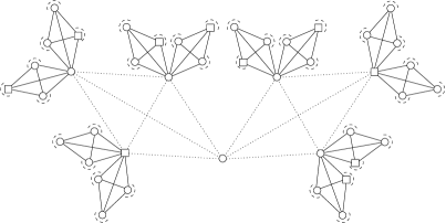
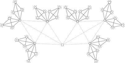
Figure 2: Possible iteration steps leading to rooted trees with root in the 0-lattice (left), 1-lattice (right). Vertices belonging to the 0-lattice (1-lattice) are depicted by $\circ$ ($\Box$). Figure from Ref. HaWe .

Let us start with a minimal set of observables. As we need an indication whether the system is liquid or crystalline, we obviously need the two sublattice particle densities $\rho^{(0)}$ and $\rho^{(1)}$ that refer to the 0-lattice and 1-lattice respectively. The normalisation is chosen such that $\rho^{(0)}\to 0$ and $\rho^{(1)}\to 1$ in the close packing limit $\mu\to\infty$. Before being able to write any closed dynamical equation for the two sublattice densities, we have to consider the generalised equilibrium ensemble defined in the last section. We introduce two chemical potentials $\mu^{(0)}$ and $\mu^{(1)}$ that couple to the particles on the respective sublattice. The calculation of $\Xi_{G}$ can be performed analogously to that of the grand partition function $\Xi(\mu)$ using the concept of rooted trees. Here we give only a shortened description of how to do so, for technical details see HaWe . A rooted tree is obtained from a generalised Bethe lattice by choosing a site as the root and removing one of the $k+1$ incident branches. Rooted trees can be iterated according to Fig. 2 where dashed lines depict the edges which are added in one iteration step. We introduce conditional partition functions $\Xi_{e}^{(0/1)}$ (resp. $\Xi_{*}^{(0/1)}$) for a subtree rooted in a 0/1-site which is fixed to be empty (resp. occupied). These quantities iterate according to

$${\Xi_{e}^{(0)}}^{\prime} = \Bigl{(}\Xi_{e}^{(0)}\bigl{(}\Xi_{e}^{(0)}\bigr{)}^{p-1}+\Xi_{*}^{(1)}\bigl{(}\Xi_{e}^{(0)}\bigr{)}^{p-1}+(p-1)\,\Xi_{e}^{(1)}\Xi_{*}^{(0)}\bigl{(}\Xi_{e}^{(0)}\bigr{)}^{p-2}\Bigr{)}^{k}$$ (i)

$${\Xi_{*}^{(0)}}^{\prime} = e^{\mu^{(0)}}\,\Bigl{(}\Xi_{e}^{(1)}\bigl{(}\Xi_{e}^{(0)}\bigr{)}^{p-1}\Bigr{)}^{k}$$ (ii)

$${\Xi_{e}^{(1)}}^{\prime} = \Bigl{(}\bigl{(}\Xi_{e}^{(0)}\bigr{)}^{p}+p\,\Xi_{*}^{(0)}\bigl{(}\Xi_{e}^{(0)}\bigr{)}^{p-1}\Bigr{)}^{k}$$ (iii)

$${\Xi_{*}^{(1)}}^{\prime} = e^{\mu^{(1)}}\,\Bigl{(}\bigl{(}\Xi_{e}^{(0)}\bigr{)}^{p}\Bigr{)}^{k}\;.$$ (iv)

The stroke labels the partition functions of the resulting large rooted tree. All 0-rooted trees that enter in the iteration are taken to be identical, the same is assumed for all 1-rooted trees. When we pass to intensive quantities by introducing local fields $x^{(0/1)}=\frac{\Xi_{*}^{(0/1)}}{\Xi_{e}^{(0/1)}}$, the strokes in Eqs. (3) drop out and the iteration equations reduce to two equations for the local fields $x^{(0/1)}$ which still contain the unknown chemical potentials $\mu^{(0/1)}$. These can be eliminated through the connection of Eqs. (3) with the observables $\rho^{(0/1)}$ which is established via the physical partition functions $\tilde{\Xi}_{e}^{(0/1)}$ and $\tilde{\Xi}_{*}^{(0/1)}$. The latter refer to a site within the generalised Bethe lattice (not the root of a subtree), i.e. they are obtained like the stroked partition functions in Eqs. (3) after the substitution $k\to k+1$ on the r.h.s. of the equations. The relations $\frac{\rho^{(0/1)}}{1-\rho^{(0/1)}}=\frac{\tilde{\Xi}_{*}^{(0/1)}}{\tilde{\Xi}_{e}^{(0/1)}}$ allow to derive two more equations, and we end up with four equations containing the four unknown $x^{(0/1)}$ and $\mu^{(0/1)}$. Their solution is straight-forward yielding

$$x^{(0/1)}=\frac{\rho^{(0/1)}}{1-\rho^{(1)}-p\,\rho^{(0)}}$$ (4)

and

$$e^{\mu^{(0/1)}}=\frac{\rho^{(0/1)}(1-\rho^{(0/1)})^{k}}{(1-\rho^{(1)}-p\,\rho^{(0)})^{k+1}}\;.$$ (5)

We note that Eq. (5) is the self-consistency result for the chemical potentials and Eq. 4 is the result for the conditional partition functions that are essentially contained in the local fields. We also mention that by setting $\mu^{(0)}=\mu^{(1)}=\mu$ the results of the calculation for the statics are recovered, i.e. we have found an “equilibrium” treatment for non-equilibrium configurations of $\rho^{(0/1)}$ that naturally contains the physical equilibrium ensemble as a special case.

In order to derive the approximative differential equations for the time-evolution of $\rho^{(0/1)}$, we start with the exact equations for the average change $\Delta N_{*}^{(0/1)}$ in the number of particles $N_{*}^{(0/1)}$ on the respective sublattice. The average is taken over the time $\Delta t=1/N$ where $N=N^{(0)}+N^{(1)}$ is the overall number of sites and $N^{(0/1)}$ are the numbers of sites belonging to the sublattices. $\Delta t$ is the time that corresponds to one action of the MC-algorithm that implements the dynamics (see Sec. II.2). The changes $\Delta N_{*}^{(0/1)}$ are given by rate-equations:

$$\Delta N_{*}^{(0/1)} = -\frac{N^{(0/1)}}{N}\,\rho^{(0/1)}\,q_{0}+\frac{N^{(0/1)}}{N}\,(1-\rho^{(0/1)})\,q_{1}\,\mathcal{P}_{1}^{(0/1)}$$ (6)

$$-\frac{N^{(0/1)}}{N}\,\rho^{(0/1)}\,q_{s}\,\mathcal{P}_{s}^{(0/1)}+\frac{N^{(1/0)}}{N}\,\rho^{(1/0)}\,q_{s}\,\mathcal{P}_{s}^{(1/0)}\;.$$

The first term on the r.h.s. corresponds to a loss due to annihilation of a particle. The three factors mean that the algorithm must choose a site on the lattice in question ($\frac{N^{(0/1)}}{N}$) which is occupied ($\rho^{(0/1)}$) and annihilate it ($q_{0}$). This contribution is exactly known. The second term contains the gain due to particle creation. Here $\mathcal{P}_{1}^{(0/1)}$ denotes the probability that the particle creation is possible without violating the hard-sphere constraint, i.e. the probability that all neighbours of the selected site on the 0/1-lattice are also empty. Its value in one microscopic (non-equilibrium) configuration cannot be expressed as a function of the $\rho^{(0/1)}$-values of this configuration, as it contains information about nearest-neighbour correlations that are not included in the single-site observables $\rho^{(0/1)}$. The third term gives the loss of particles caused by those that jump to the other sublattice whereas the last term contains the gain of particles caused by those that jump from the other sublattice to the sublattice under consideration. Hereby, $\mathcal{P}_{s}^{(0/1)}$ denotes the probability that a tried move of a particle on the 0/1-lattice to a neighbouring site on the 1/0-lattice is in fact feasible. This is again a quantity which involves neighbour correlations and cannot be expressed exactly for one configuration given only by $\rho^{(0/1)}$.

In order to close Eq. (6) we now proceed to the last step mentioned in the outline of PAS. We have to calculate the probabilities $\mathcal{P}_{\cdot}^{(0/1)}$ within the pseudo-equilibrium ensemble characterised by the already determined formal chemical potentials $\mu^{(0/1)}$, i.e. the $\mathcal{P}_{\cdot}^{(0/1)}$ are calculated via a flat average over all configurations having the desired values of $\rho^{(0/1)}$. For instance, we can calculate

$$\mathcal{P}_{1}^{(0)} = \frac{\overbrace{\Bigl{(}\Xi_{e}^{(1)}\bigl{(}\Xi_{e}^{(0)}\bigr{)}^{p-1}\Bigr{)}^{k+1}}^{\text{all neighbouring sites are empty}}}{\underbrace{\Bigl{(}\Xi_{e}^{(1)}\bigl{(}\Xi_{e}^{(0)}\bigr{)}^{p-1}+\Xi_{*}^{(1)}\bigl{(}\Xi_{e}^{(0)}\bigr{)}^{p-1}+(p-1)\,\Xi_{e}^{(1)}\Xi_{*}^{(0)}\bigl{(}\Xi_{e}^{(0)}\bigr{)}^{p-2}\Bigr{)}^{k+1}}_{\text{no requirements to the neighbouring sites}}}$$ (7)

$$= \frac{1}{\bigl{(}1+x^{(1)}+(p-1)\,x^{(0)}\bigr{)}^{k+1}}$$

$$\overset{\text{\eqref{gl_x01approx}}}{=} \left(\frac{1-\rho^{(1)}-p\,\rho^{(0)}}{1-\rho^{(0)}}\right)^{k+1}\;.$$

Similarly we find

$$\mathcal{P}_{1}^{(1)}=\left(\frac{1-\rho^{(1)}-p\,\rho^{(0)}}{1-\rho^{(1)}}\right)^{k+1}\;.$$ (8)

For the calculation of $\mathcal{P}_{s}^{(0)}$ we must consider that, starting from a 0-site, only $k+1$ of the $(k+1)p$ neighbouring sites belong to the 1-lattice which is taken into account with a factor $\frac{1}{p}$. Furthermore we know that the ending site of the jump is empty as are all other sites in the clique that is shared by starting site and ending site. The only condition for $\mathcal{P}_{s}^{(0)}$ is that the $kp$ sites of the $k$ other cliques containing the ending site are empty. These sites are all in the 0-lattice as the ending site is in the 1-lattice. This leads to

$$\mathcal{P}_{s}^{(0)}=\frac{1}{p}\>\frac{\Bigl{(}\bigl{(}\Xi_{e}^{(0)}\bigr{)}^{p}\Bigr{)}^{k}}{\Bigl{(}\bigl{(}\Xi_{e}^{(0)}\bigr{)}^{p}+p\,\Xi_{*}^{(0)}\bigl{(}\Xi_{e}^{(0)}\bigr{)}^{p-1}\Bigr{)}^{k}}=\frac{1}{p}\>\left(\frac{1-\rho^{(1)}-p\,\rho^{(0)}}{1-\rho^{(1)}}\right)^{k}$$ (9)

and similarly

$$\mathcal{P}_{s}^{(1)}=\left(\frac{1-\rho^{(1)}-p\,\rho^{(0)}}{1-\rho^{(0)}}\right)^{k}\;.$$ (10)

These approximations close Eq. (6). We add that

$$\Delta N_{*}^{(0/1)}=\frac{N^{(0/1)}}{N}\,\frac{\Delta(N_{*}^{(0/1)}/N^{(0/1)})}{\Delta t}=\frac{N^{(0/1)}}{N}\,\frac{\Delta\rho^{(0/1)}}{\Delta t}$$ (11)

and

$$\frac{N^{(0)}}{N}=\frac{p}{p+1}\,,\qquad\frac{N^{(1)}}{N}=\frac{1}{p+1}\;.$$ (12)

for the generalised Bethe lattice.

Using these ingredients, in the thermodynamic limit $N\to\infty$ Eq. (6) becomes:

$$\dot{\rho}^{(0)}= -\rho^{(0)}\,q_{0}+(1-\rho^{(0)})\,q_{1}\,\left(\frac{1-\rho^{(1)}-p\,\rho^{(0)}}{1-\rho^{(0)}}\right)^{k+1}$$

$$-\rho^{(0)}\,q_{s}\,\frac{1}{p}\,\left(\frac{1-\rho^{(1)}-p\,\rho^{(0)}}{1-\rho^{(1)}}\right)^{k}+\rho^{(1)}\,q_{s}\,\frac{1}{p}\,\left(\frac{1-\rho^{(1)}-p\,\rho^{(0)}}{1-\rho^{(0)}}\right)^{k}$$ (i)

and

$$\dot{\rho}^{(1)}= -\rho^{(1)}\,q_{0}+(1-\rho^{(1)})\,q_{1}\,\left(\frac{1-\rho^{(1)}-p\,\rho^{(0)}}{1-\rho^{(1)}}\right)^{k+1}$$

$$-\rho^{(1)}\,q_{s}\,\left(\frac{1-\rho^{(1)}-p\,\rho^{(0)}}{1-\rho^{(0)}}\right)^{k}+\rho^{(0)}\,q_{s}\,\left(\frac{1-\rho^{(1)}-p\,\rho^{(0)}}{1-\rho^{(1)}}\right)^{k}\,.$$ (ii)

Eqs. (13) constitute what we call the $\rho$-approximation, i.e. the approximation for the crystallisation dynamics which is derived for a minimal set of observables – $\rho^{(0)}$ and $\rho^{(1)}$ – in the context of PAS. The approximative time-flow of $\rho^{(0/1)}$ can be obtained for given initial conditions by integrating Eqs. (13) numerically. Results are shown in Sec. IV.3 where the $\rho$-approximation and $\sigma_{j}$-approximation are compared with MC simulations.

Asymptotics of the $\rho$-approximation

Exactly at the stationary point of these equations, corresponding to an equilibrium solution of the model, the assumption of the PAS becomes true. The stationary points of Eqs. (13) are therefore identical to the static liquid and crystalline solutions discussed in Ref. HaWe .

A linear expansion of Eqs. (13) therefore allows to analyse the stability of the equilibrium solution as well as to determine the equilibration time. To achieve this, we have to calculate the Jacobian of the above system of equations,

$$A\overset{.}{=}\left(\begin{array}[]{cc}\frac{\partial\dot{\rho}^{(0)}}{\partial\rho^{(0)}}&\frac{\partial\dot{\rho}^{(0)}}{\partial\rho^{(1)}}\\ \frac{\partial\dot{\rho}^{(1)}}{\partial\rho^{(0)}}&\frac{\partial\dot{\rho}^{(1)}}{\partial\rho^{(1)}}\end{array}\right)\ .$$ (14)

This matrix has to be evaluated at the stationary point. Let us assume that it has the two eigenvalues $\lambda_{1}$ and $\lambda_{2}$ with corresponding eigenvectors $\vec{v}_{1}$ and $\vec{v}_{2}$. The time evolution of a small perturbation around the stationary point is then given by

$$\Biggl{(}\begin{array}[]{c}\rho^{(0)}(t)\\ \rho^{(1)}(t)\end{array}\Biggr{)}=\Biggl{(}\begin{array}[]{c}\rho^{(0)}_{\text{stat}}\\ \rho^{(1)}_{\text{stat}}\end{array}\Biggr{)}+\alpha_{1}\,e^{\lambda_{1}t}\,\vec{v}_{1}+\alpha_{2}\,e^{\lambda_{2}t}\,\vec{v}_{2}$$ (15)

with constants $\alpha_{1}$ and $\alpha_{2}$ which follow from the initial condition, i.e. from the specific form of the perturbation.

The stationary point is obviously stable if both eigenvalues $\lambda_{1}$ and $\lambda_{2}$ are negative. In this case, the equilibration time is given by $\tau_{eq}=-1/\max\{\lambda_{1},\lambda_{2}\}$. If at least one of the eigenvectors is positive, the stationary point is unstable and thus physically irrelevant: Any small perturbation having a component in the direction of the corresponding eigenvector carries the system exponentially fast away from the stationary point.

Let us first consider the liquid solution, which is characterised by equal sublattice densities $\rho^{(0)}=\rho^{(1)}=\rho$. In this case, the eigenvalues can be given in a compact form:

$$\lambda_{1} = -\frac{q_{1}\bigl{(}1+\rho(kp-1)\bigr{)}}{e^{\mu}\bigl{(}1-(p+1)\rho\bigr{)}\bigl{(}1-\rho\bigr{)}}$$ (i)

$$\lambda_{2} = -\frac{\bigl{(}1-(k+1)\rho\bigr{)}\bigl{(}q_{1}p+\rho(p+1)(q_{s}-q_{1}p)\bigr{)}}{e^{\mu}\,p\,\bigl{(}1-(p+1)\rho\bigr{)}\bigl{(}1-\rho\bigr{)}}\,$$ (ii)

and the eigenvectors are

$$\vec{v}_{1}=\biggl{(}\begin{array}[]{c}1\\ 1\end{array}\biggr{)}\,,\qquad\qquad\vec{v}_{2}=\biggl{(}\begin{array}[]{c}1\\ -p\end{array}\biggr{)}\,.$$ (17)

Both eigenvectors are negative for low densities, but $\lambda_{2}$ changes sign at $\rho_{cr}=\frac{1}{k+1}$. This point coincides with the local instability of the liquid state in the statical calculation of HaWe .

It is also interesting to look at the equilibration time $\tau_{eq}=-1/\max\{\lambda_{1},\lambda_{2}\}$. For small chemical potential $\mu$, the latter is given by $-1/\lambda_{1}$. Looking at the eigenvector $\vec{v}_{1}$, we see that the corresponding slowest equilibration process in the system describes the decay of global density fluctuations. Close to the instability point of the liquid solution, we find, however, $\tau_{eq}=-1/\lambda_{2}$, and the eigenvector indicates that the slowest decaying perturbation is a difference in the two sublattice densities, i.e. a fluctuation toward a crystalline state. At a certain $\mu=\mu_{eq}$ the two eigenvectors are equal. At this point, a crossover between the two different slowest processes takes place. It is also the point, where the equilibration time takes its minimum inside the liquid phase, i.e. where the system equilibrates faster than for any other $\mu<\mu_{cr}$, see also the discussion in Sec. IV.3, where these analytical results are compared with MC simulations.

Let us now discuss the stability of the two crystalline solutions calculated in HaWe . The determinant of the Jacobian matrix $A$ vanishes at the point where the crystalline solution appears.

• For $p=1$, i.e. on the ordinary Bethe lattice, the two crystalline solutions appear continuously out of the liquid solution, and they become both stable, marking thus a second-order transition. The two solutions are in fact identical, they are related by an exchange of the two sub-lattices which are isomorphic for $p=1$.

• For $p>1$, the two crystalline solutions appear discontinuously. The normal crystalline solution, i.e. the one with higher total density, becomes immediately locally stable, both eigenvalues of the Jacobian matrix are negative. The second solution is first locally unstable and thus unphysical. At $\mu=\mu_{cr}$, the two sublattice densities cross, however, at the value $\rho_{cr}=\frac{1}{k+1}$, and thus coincide with the liquid solution. For higher $\mu$ we have $\rho_{0}>\rho_{1}$, in HaWe we have introduced the name “inverse crystallisation” for this phenomenon. This solution takes over the local stability of the liquid solution as can be inferred from the eigenvalues of $A$.

It is also possible to analytically characterise the critical behaviour close to $\mu_{cr}$, which is, on both sides of the transition, characterised by a critical exponent $-1$:

$$\tau_{eq}\propto|\mu-\mu_{cr}|^{-1}\ .$$ (18)

We skip the calculation of the prefactors here, we only mention that in the case $p=1$ both sides of the transition are related by an universal factor $1/2$, as already found in the case of a simple ferromagnet on a Bethe lattice SeWe . Further results are given below in the context of the comparison between analytical and numerical data.

IV.2 The $\sigma_{j}$-approximation

The $\rho$-approximation was derived according to PAS using the pure single-site observables $\rho^{(0/1)}$. There we have seen that it was necessary to approximate nearest-neighbour correlations within the generalised ensemble. We now go over to more detailed observables including also such nearest-neighbour correlations. This can be achieved by defining

$$\sigma_{j}^{(0/1)}$$:= density of sites on the 0/1-lattice which are empty and have exactly occupied neighbouring sites, .

(19)

Note that the $\sigma_{j}^{(0/1)}$ imply the previous observables via $\rho^{(0/1)}=1-\sum_{j=0}^{k+1}\sigma_{j}^{(0/1)}$. Therefore they allow for an exact characterisation of the liquid and crystalline equilibrium states, and according to the rule of our PAS they represent a valid set of observables.

Again, we apply PAS introducing formal chemical potentials $\mu_{j}^{(0/1)}$, $j=0,\ldots,k+1$, being conjugated to the $\sigma_{j}^{(0/1)}$. This allows to calculate conditional partition functions $\Xi_{j}^{(0/1)}$, $j=0,\ldots,k$ which stand for a 0/1-rooted tree with an empty root having $j$ occupied neighbouring sites, and $\Xi_{*}^{(0/1)}$ which stands for a 0/1-rooted tree with occupied root. The iteration of rooted trees (see Fig. 2) reads in terms of the conditional partition functions:

$${\Xi_{*}^{(0)}}^{\prime} = \Biggl{\{}\biggl{(}\sum_{l=0}^{k}e^{\mu_{l+1}^{(1)}}e^{-\mu_{l}^{(1)}}\Xi_{l}^{(1)}\biggr{)}\biggl{(}\sum_{l=0}^{k}e^{\mu_{l+1}^{(0)}}e^{-\mu_{l}^{(0)}}\Xi_{l}^{(0)}\biggr{)}^{p-1}\Biggr{\}}^{k}\,,$$ (i)

$${\Xi_{j}^{(0)}}^{\prime} = e^{\mu_{j}^{(0)}}{k\choose j}\Biggl{\{}\Xi_{*}^{(1)}\biggl{(}\sum_{l=0}^{k}e^{\mu_{l+1}^{(0)}}e^{-\mu_{l}^{(0)}}\Xi_{l}^{(0)}\biggr{)}^{p-1}$$ (ii)

$$\hskip 56.9055pt+(p-1)\,\Xi_{*}^{(0)}\biggl{(}\sum_{l=0}^{k}e^{\mu_{l+1}^{(1)}}e^{-\mu_{l}^{(1)}}\Xi_{l}^{(1)}\biggr{)}\biggl{(}\sum_{l=0}^{k}e^{\mu_{l+1}^{(0)}}e^{-\mu_{l}^{(0)}}\Xi_{l}^{(0)}\biggr{)}^{p-2}\Biggr{\}}^{j}\times$$

$$\hskip 33.57404pt\times\>\Biggl{\{}\biggl{(}\sum_{l=0}^{k}\Xi_{l}^{(1)}\biggr{)}\biggl{(}\sum_{l=0}^{k}\Xi_{l}^{(0)}\biggr{)}^{p-1}\Biggr{\}}^{k-j}$$

and

$${\Xi_{*}^{(1)}}^{\prime} = \Biggl{\{}\biggl{(}\sum_{l=0}^{k}e^{\mu_{l+1}^{(0)}}e^{-\mu_{l}^{(0)}}\Xi_{l}^{(0)}\biggr{)}^{p}\Biggr{\}}^{k}\,,$$ (iii)

$${\Xi_{j}^{(1)}}^{\prime} = e^{\mu_{j}^{(1)}}{k\choose j}\Biggl{\{}p\,\Xi_{*}^{(0)}\biggl{(}\sum_{l=0}^{k}e^{\mu_{l+1}^{(0)}}e^{-\mu_{l}^{(0)}}\Xi_{l}^{(0)}\biggr{)}^{p-1}\Biggr{\}}^{j}\times\Biggl{\{}\biggl{(}\sum_{l=0}^{k}\Xi_{l}^{(0)}\biggr{)}^{p}\Biggr{\}}^{k-j}\,.$$ (iv)

The stroked partition functions belong to the rooted tree that results from the iteration. We shall only explain the structure of Eq. (ii) exemplarily. It describes the situation where the root of the resulting tree is in the 0-lattice (see Fig. 2 left) and empty with $j$ occupied neighbouring sites. The exponential prefactor accounts for the addition of a site of this kind. The binomial factor counts the possibilities to distribute the $j$ particles on the $k$ adjacent branches. The first curly brackets refer to the situation of a branch containing a particle. This particle can sit on the 1-lattice (first term in the brackets, $\Xi_{*}^{(1)}$). The factor following $\Xi_{*}^{(1)}$ expresses the possibilities for empty sites with a given number of occupied neighbours on the other $p-1$ sites of the clique. Note that the factor $e^{\mu_{l+1}^{(0)}}e^{-\mu_{l}^{(0)}}$ is due to the particle present on the 1-site of the clique which increases the number of occupied neighbours for the empty 0-sites by one. The second term in the brackets stands for the $p-1$ possibilities of placing the particle on a 0-site. The second curly brackets refer to an empty clique. All possible combinations of empty sites with $l=0,\ldots,k$ occupied neighbouring sites are included.

For the calculation of the partition functions we follow the same lines as for Eqs. (3). We introduce intensive quantities with the local fields

$$x_{j}^{(0/1)}=\frac{\Xi_{j}^{(0/1)}}{\Xi_{*}^{(0/1)}}\>,\quad j=0,\ldots,k\,.$$ (21)

By taking the ratio of Eq. (ii) and Eq. (i) as well as Eq. (iv) and Eq. (iii) for $j=0,\ldots,k$ we obtain $2(k+1)$ equations for these local fields that still contain the $2(k+2)$ chemical potentials. These can be eliminated via the introduction of physical partition functions $\tilde{\Xi}_{j}^{(0/1)}$, $j=0,\ldots,k+1$ and $\tilde{\Xi}_{*}^{(0/1)}$ which replace the stroked quantities in Eqs. (20) after substitution of $k\to k+1$ in the binomials and exponents. By taking the ratios of Eqs. (20) as before but for $j=0,\ldots,k+1$ and using that $\frac{\tilde{\Xi}_{j}^{(0/1)}}{\tilde{\Xi}_{*}^{(0/1)}}=\frac{\sigma_{j}^{(0/1)}}{\rho^{(0/1)}}$ we obtain $2(k+2)$ more equations, so that we end up with the same number of equations and unknown local fields and chemical potentials.

The solution of the corresponding equations for the $\rho$-approximation was obtained by simple algebra which seems not possible in the present case considering the complexity of the equations. We can, however, show that the ansatz

$$x_{j}^{(0/1)} = \alpha^{(0/1)}\,\frac{k+1-j}{k+1}\,\sigma_{j}^{(0/1)}\,,$$ (i)

$$e^{\mu_{j+1}^{(0/1)}}e^{-\mu_{j}^{(0/1)}}x_{j}^{(0/1)} = \beta^{(0/1)}\,\frac{j+1}{k+1}\,\sigma_{j+1}^{(0/1)}$$ (ii)

with $j=0,\ldots,k$ solves the equations under certain conditions. One of coefficients $\alpha^{(0/1)}$ and $\beta^{(0/1)}$ can be chosen arbitrarily for each sublattice. These two extra degrees of freedom arise from the consistency conditions that must be imposed for the validity of Ansatz (22) and which read

$$\rho^{(0)}=\frac{1}{p}\,\sum_{l=0}^{k}\frac{l+1}{k+1}\,\sigma_{l+1}^{(1)}\,,\qquad\rho^{(1)}=\sum_{l=0}^{k}\frac{l+1}{k+1}\,\sigma_{l+1}^{(0)}-\frac{p-1}{p}\,\sum_{l=0}^{k}\frac{l+1}{k+1}\,\sigma_{l+1}^{(1)}$$ (23)

and which reduce the independent observables by one for each sublattice. Eqs. (23) can be easily understood through the observation that, e.g., empty sites on the 1-lattice with occupied neighbouring sites contribute to the particle density on the 0-lattice (first equation). Eqs. (23) are indeed important conditions as they assure that a choice of $\sigma_{j}^{(0/1)}$ is realisable within a microscopic configuration, and thus they do not imply any restriction of Ansatz (22) for physically relevant situations.

As in Sec. IV.1 we now derive the differential equations for the time evolution of the observables. Unknown probabilities are again approximated by their pseudo-equilibrium values in the ensemble characterised by $\Xi_{G}$. A complete list of the contributions due to the different actions of the dynamics is given in Appendix A. We shall only discuss the case of the jump from a 0-site to a 1-site which qualitatively includes the calculations occurring in all other cases.

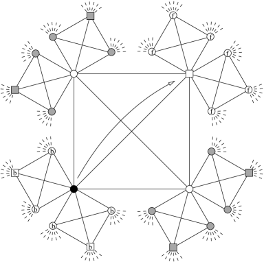
Figure 3: Sketch for the jump from a 0-site to a 1-site ($k=2,p=3$).

The occurrence of a 0-1-jump requires that the algorithm selects a 0-site (1) which is occupied (2) and the decision to try a jump must be made (3) in favour of an ending site which is in the 1-lattice (4). The probability is given by $(1)\cdot(2)\cdot(3)\cdot(4)=\frac{p}{p+1}\cdot\rho^{(0)}\cdot q_{s}\cdot\frac{1}{p}$. It remains to calculate the probability that in the above situation the jump will be successful. To this purpose we introduce the quantity $\Xi_{e}^{\prime(0/1)}=\sum_{l=0}^{k}e^{\mu_{l+1}^{(0/1)}}e^{-\mu_{l}^{(0/1)}}\Xi_{l}^{(0/1)}$ which corresponds to a rooted tree with an empty root but with the modification that one extra occupied site is connected to the root (empty sites connected to the root will not alter the expression). Then the situation where (1) to (4) holds can be described by

$$\Xi_{*}^{(0)}\,(\Xi_{e}^{\prime(0)})^{p-1}\,\Xi_{e}^{\prime(1)}\,,$$ (24)

in terms of conditional partition functions. The situation is depicted in Fig. 3 where for grey sites it is not known whether they are empty or occupied. For a successful jump we must require all sites labelled with f to be empty. This is a restriction of the above situation which reads in terms of conditioned partition functions:

$$\Xi_{*}^{(0)}\,(\Xi_{e}^{\prime(0)})^{p-1}\,e^{\mu_{1}^{(1)}}e^{-\mu_{0}^{(1)}}\Xi_{0}^{(1)}\,.$$ (25)

The ratio of Eqs. (25) and (24) gives the probability that the jump can actually be performed:

$$\frac{\Xi_{*}^{(0)}\,(\Xi_{e}^{\prime(0)})^{p-1}\,e^{\mu_{1}^{(1)}}e^{-\mu_{0}^{(1)}}\Xi_{0}^{(1)}}{\Xi_{*}^{(0)}\,(\Xi_{e}^{\prime(0)})^{p-1}\,\Xi_{e}^{\prime(1)}}=\frac{e^{\mu_{1}^{(1)}}e^{-\mu_{0}^{(1)}}\Xi_{0}^{(1)}}{\sum_{l=0}^{k}e^{\mu_{l+1}^{(1)}}e^{-\mu_{l}^{(1)}}\Xi_{l}^{(1)}}$$ (26)

$$= \frac{e^{\mu_{1}^{(1)}}e^{-\mu_{0}^{(1)}}x_{0}^{(1)}}{\sum_{l=0}^{k}e^{\mu_{l+1}^{(1)}}e^{-\mu_{l}^{(1)}}x_{l}^{(1)}}\overset{\text{\eqref{gl_sigmajloes1}}}{=}\frac{\frac{1}{k+1}\sigma_{1}^{(1)}}{\sum_{l=0}^{k}\frac{l+1}{k+1}\,\sigma_{l+1}^{(1)}}\,.$$

We shall now discuss the contributions of the 0-1-jump to the changes in the $\sigma_{j}^{(0/1)}$ which we divide in three classes. The first class contains the intra-clique contributions which are all contributions coming from sites in the clique where the jump takes place (i.e. the central clique in Fig. 3). For the $(p-1)$ empty 0-sites in this clique the number of occupied neighbouring sites remains unaltered through the jump. A non-zero intra-clique contribution is due to the occupied 0-site. After the jump, this site is empty with exactly one occupied neighbouring site which means that the number of sites corresponding to $\sigma_{1}^{(0)}$ must be increased by one. The second intra-clique contribution stems from the ending site which has one occupied neighbour before the jump but becomes an occupied site after the jump. This means we must decrease the number of vacancies corresponding to $\sigma_{1}^{(1)}$ by one.

The second class of contributions will be termed as backward contributions. They stem from the neighbouring sites which the particle leaves behind during the jump (labelled with b in Fig. 3). The backward 0-sites may have $j=0,\ldots,k$ occupied neighbours in addition to the jumping particle. The corresponding sites are not shown in Fig. 3, only the edges are drawn as dashed lines. We will have a positive contribution to $\sigma_{j}^{(0)}$ from the sites having $j$ occupied neighbours in addition to the jumping particle. The same contribution with a negative sign must be attributed to $\sigma_{j+1}^{(0)}$. In order to quantify the contribution, we need to calculate the expected number of backward sites with $j$ extra neighbours. For the calculation we define the partition function $\Xi_{*,\nu_{j}}^{(0)}$ which refers to a 0-rooted tree with occupied root having exactly $\nu_{j}$ neighbouring 0-sites with $j$ extra occupied neighbours. The quantity is given by

$$\Xi_{*,\nu_{j}}^{(0)}={k(p-1)\choose\nu_{j}}\biggl{(}\sum_{l=0}^{k}e^{\mu_{l+1}^{(1)}}e^{-\mu_{l}^{(1)}}\Xi_{l}^{(1)}\biggr{)}^{k}\Bigl{(}e^{\mu_{j+1}^{(0)}}e^{-\mu_{j}^{(0)}}\Xi_{j}^{(0)}\Bigr{)}^{\nu_{j}}\biggl{(}\sum_{\begin{subarray}{c}l=0\\ l\neq j\end{subarray}}^{k}e^{\mu_{l+1}^{(0)}}e^{-\mu_{l}^{(0)}}\Xi_{l}^{(0)}\biggr{)}^{k(p-1)-\nu_{j}}\,.$$ (27)

The average number of backward 0-sites with $j$ additional occupied neighbours is then given by

$$\sum_{\nu_{j}=0}^{k(p-1)}\nu_{j}\,\frac{\Xi_{*,\nu_{j}}^{(0)}}{{\Xi_{*}^{(0)}}^{\prime}}=k(p-1)\,\frac{\frac{j+1}{k+1}\,\sigma_{j+1}^{(0)}}{\sum_{l=0}^{k}\frac{l+1}{k+1}\,\sigma_{l+1}^{(0)}}\,.$$ (28)

Here ${\Xi_{*}^{(0)}}^{\prime}$ serves as a normalisation as it corresponds to the unconstrained scenario. The r.h.s. is obtained by substitution of ${\Xi_{*}^{(0)}}^{\prime}$ and $\Xi_{*,\nu_{j}}^{(0)}$ according to Eqs. (i) and (27) and performing the summation. With this result the backward contribution of the 0-sites can be easily expressed (see Appendix A). The calculation of the backward contribution of the 1-sites follows very similar lines yielding an average number of backward 1-sites with $j$ additional occupied neighbouring sites which is

$$k\,\frac{\frac{j+1}{k+1}\,\sigma_{j+1}^{(1)}}{\sum_{l=0}^{k}\frac{l+1}{k+1}\,\sigma_{l+1}^{(1)}}\,.$$ (29)

A third class contains the forward contributions which come from the sites labelled with f in Fig. 3. The f-sites having exactly $j-1$ occupied neighbouring sites will yield a positive contribution to $\sigma_{j}^{(0)}$ and a negative contribution comes from the f-sites with exactly $j$ occupied neighbouring sites. The average number of f-sites with exactly $j$ occupied neighbouring sites can be calculated with the help of the corresponding partition function

$$\Xi_{0,\nu_{j}}^{(1)}=e^{\mu_{0}^{(1)}}{kp\choose\nu_{j}}\Bigl{(}\Xi_{j}^{(0)}\Bigr{)}^{\nu_{j}}\biggl{(}\sum_{\begin{subarray}{c}l=0\\ l\neq j\end{subarray}}^{k}\Xi_{l}^{(0)}\biggr{)}^{kp-\nu_{j}}\,.$$ (30)

One obtains the average number as

$$\sum_{\nu_{j}=0}^{kp}\nu_{j}\,\frac{\Xi_{0,\nu_{j}}^{(1)}}{{\Xi_{0}^{(1)}}^{\prime}}=kp\,\frac{\frac{k+1-j}{k+1}\,\sigma_{j}^{(0)}}{\sum_{l=0}^{k}\frac{k+1-l}{k+1}\,\sigma_{l}^{(0)}}\,.$$ (31)

With similar arguments all the contributions can be derived (for the results see Appendix A) and one ends up with a system of $2(k+2)$ differential equations which is of the form

$$\dot{\sigma}_{j}^{(\iota)}=\dot{\sigma}_{j}^{(\iota)}\bigl{(}\sigma_{0}^{(0)},\ldots,\sigma_{k+1}^{(0)};\sigma_{0}^{(1)},\ldots,\sigma_{k+1}^{(1)}\bigr{)}\,,$$ (32)

with $j=0,\ldots,k+1$ and $\iota=0,1$.

For given initial conditions $\rho^{(0)}(t=0)=\rho^{(0)}$ and $\rho^{(1)}(t=0)=\rho^{(1)}$ we first calculate the initial values $\sigma_{j}^{(0/1)}(t=0)$ which can be performed following similar lines to the calculation of $(1-\rho^{(0/1)})\mathcal{P}_{1}^{(0/1)}$ (see Sec. IV.1, Eq. (7)). $(1-\rho^{(0/1)})\mathcal{P}_{1}^{(0/1)}$ is the probability for an empty site without occupied neighbouring sites which is obviously equivalent to $\sigma_{0}^{(0/1)}$. A more general calculation yields, for $j=0,\ldots,k+1$,

$$\sigma_{j}^{(0/1)}(t=0)\,=\,\bigl{(}1-\rho^{(0/1)}\bigr{)}{k+1\choose j}\left(1-\frac{1-\rho^{(1)}-p\,\rho^{(0)}}{1-\rho^{(0/1)}}\right)^{j}\left(\frac{1-\rho^{(1)}-p\,\rho^{(0)}}{1-\rho^{(0/1)}}\right)^{k+1-j}\ .$$ (33)

With these initial values, the $\sigma_{j}$-approximation is obtained by integrating Eqs. (32) numerically. We add that the conditions (23) are fulfilled by the initial values and preserved by Eqs. (32).

Eqs. (32) can be evaluated asymptotically as this was done analytically for the $\rho$-approximation in Sec. IV.1. The Jacobian matrix $A$ of the system is a $2(k+2)\times 2(k+2)$-matrix:

$$A=\left(\begin{array}[]{cc}A_{00}&A_{01}\\ A_{10}&A_{11}\end{array}\right)\,,\qquad\text{where}\quad A_{mn}=\left(\begin{array}[]{ccc}\frac{\partial\dot{\sigma}_{0}^{(m)}}{\partial\sigma_{0}^{(n)}}&\ldots&\frac{\partial\dot{\sigma}_{0}^{(m)}}{\partial\sigma_{k+1}^{(n)}}\\ \vdots&\vdots&\vdots\\ \frac{\partial\dot{\sigma}_{k+1}^{(m)}}{\partial\sigma_{0}^{(n)}}&\ldots&\frac{\partial\dot{\sigma}_{k+1}^{(m)}}{\partial\sigma_{k+1}^{(n)}}\end{array}\right)\,.$$ (34)

The matrix can be calculated with the help of a computer algebra system as well as its evaluation at a stationary points of Eqs. (32) can be done. We find that two eigenvalues always vanish which is due to the conditions (23) that reduce the effective number of observables by two. If the other eigenvalues $\{\lambda_{i}\}$ are all negative, the stationary point is stable and the inverse relaxation time is given by $\tau^{-1}=-\max\{\lambda_{i}\}$.

In the next section we show results for relaxation times and for the time-flow of the observables according to the $\rho$-approximation and $\sigma_{j}$-approximation.

IV.3 Comparison with MC simulations

As the exact dynamics is not accessible so far, there is no intrinsic way to check the quality of the results obtained according to the PAS. We therefore performed MC simulations implementing the dynamics defined in Sec. II.2 on large graphs, details of the generation of the graphs were already given in HaWe .

Equilibration time

As a first example, we look at the relaxation time for a system with $k=2$ and $p=1$, i.e. on an ordinary Bethe lattice with coordination number three. On this lattice, due to $p=1$, the crystallisation transition is of second order. The simulations where performed for an average annihilation rate $q_{0}=0.2$ and a mobility of $q_{s}=0.8$. The parameter $q_{1}$ was used to tune the chemical potential $\mu$ according to the condition (2) of detailed balance.

Let us shortly discuss the results of the analytical $\rho$-approximation for these parameters. For very diluted systems ($q_{1}\to 0,\ \mu\to-\infty$), the relaxation time goes to $1/q_{0}$. For increasing $\mu$ the relaxation time decreases until it reaches a local minimum at $\mu_{eq}\simeq-0.445$, the point where the slowest process changes from being the decay of global density fluctuations to the decay of differences between the sublattice densities. The equilibration time starts to grow until it diverges as $|\mu-\mu_{cr}|^{-1}$ if we approach the critical point $\mu_{cr}\simeq 1.383$. It restarts to decrease and at the end saturates at $1/\tau_{eq}(\mu\to\infty)=q_{0}+q_{s}/p$ which equals one for the above choice of parameters.

The $\sigma_{j}$-approximation leads to qualitatively similar, but quantitatively slightly different results: It starts at the same value of the equilibration time for $\mu\to-\infty$, but reaches the local minimum already at $\mu_{eq}\simeq-0.556$. The behaviour close to the phase transition is extremely similar, with a slightly different prefactor to the dominant critical divergence. At large chemical potentials, we have $1/\tau_{eq}(\mu\to\infty)=\frac{3}{4}q_{0}+q_{s}=0.95$, i.e. the equilibration time in the vicinity of the closest packing is slightly larger than predicted by the simpler approximation.

Figure 4: Inverse relaxation time for $q_{0}=0.2$ and $q_{s}=0.8$. The dashed line shows the results of the $\rho$-approximation, the full line those of the $\sigma_{j}$-approximation. MC data is represented by the symbols. The right figure enlarges the critical region to show the linear vanishing of $1/\tau$. The slopes on both sides of the transition are related by a factor two.

For comparison, we have plotted these results together with numerical data in Fig. 4. The numerical simulations were performed on a large bipartite lattice of $N=5\cdot 10^{6}$ sites, as an initial condition we have chosen one densest packing, the data were averaged over 10 independent runs. For extracting the equilibration time, we have plotted the logarithm of the difference $\rho^{(1)}(t)-\rho^{(1)}_{stat}$ from the analytically known equilibrium value, as a function of the MC time. The function was linearised in a suitable region. The problem hereby is to identify this region: For short times, the system is still far from its asymptotic behaviour, for large time the dynamics is dominated by fluctuations. The estimated error of this procedure grows up to 10% for the values close to the transition point.

Fig. 4 demonstrates that both approximations show a very good qualitative agreement with the numerical findings. The more detailed $\sigma_{j}$-approximation gives, however, the better quantitative values which, within the estimated error, almost coincide with the MC results.

Equilibration of the sublattice densities

As a further comparison we have investigated the relaxation of the sublattice densities for a system with $k=3$ and $p=2$. We have performed the numerical experiments on a graph of $N=4.5\cdot 10^{6}$ vertices, and have chosen the dynamical parameters as $q_{1}=1$, $q_{0}=e^{-2}$ and $q_{s}=1-q_{0}$. These values correspond to a chemical potential $\mu=2$ which is situated in the interval where the liquid as well as the normal crystalline phase are locally stable.

Figure 5: Global density for two systems ($k=3$, $p=2$) with initial conditions $\rho^{(0)}(t=0)=0$ and $\rho^{(1)}(t=0)=0.145$ (experiment A) resp. $\rho^{(1)}(t=0)=0.160$ (experiment B). The asymptotically reached densities are those of the two metastable states of the system, the smaller one corresponding to the liquid, the larger one to the crystalline phase. Numerical data was averaged over 100 runs.

We have chosen two slightly different initial conditions, in both cases the $0$-sublattice was empty. The $1$-sublattice was first initialised with a partial density $\rho^{(1)}(t=0)=0.145$ (experiment A), in the second case with $\rho^{(1)}(t=0)=0.160$ (experiment B). After a similar evolution in the initial time interval, the systems approach the two different locally stable solutions of the model. Whereas the less dense one converges to the liquid solution, the denser one crystallises. The local stability of the liquid phase is demonstrated impressively in case A: After an initial increase, the global density falls again toward the liquid value.

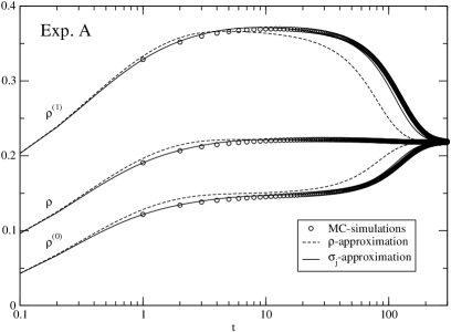
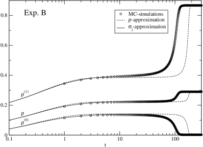
Figure 6: Global and sublattice densities for the two approximations and the MC simulation. For the corresponding initial conditions see caption of Fig. 5.

In Fig. 6, the numerical results for the global and both sublattice densities are compared to the $\rho$- and the $\sigma_{j}$-approximation. As in the case of the equilibration times, both approximations reflect correctly the qualitative behaviour. The simpler $\rho$-approximation, however, shows a rather pronounced difference in the onset of the final relaxation toward the stationary point. This is almost completely cured by the more involved $\sigma_{j}$-approximation, which shows a quantitatively impressing agreement with the MC data over the whole time interval.

V Dynamics at the glass-transition

The aim of this section is to detect also the glass-transition in the context of PAS, i.e. through its impact on time-dependent, dynamical quantities. Apparently, the observables considered so far (essentially particle densities) are not suitable to probe the fundamental difference between the liquid and amorphous state. This is clear as, e.g., the difference between the liquid solution densities and the 1RSB solution densities is hardly significant at least for an amorphous system in proximity to the glass-transition. It seems more promising to focus on the long lifetime of arrested configurations in the glassy state which obviously strongly affects the two-time autocorrelation function

$$C(t_{1},t_{2})=\frac{1}{N}\sum_{i=1}^{N}\delta_{n_{i}(t_{1}),n_{i}(t_{2})}\quad,\qquad t_{1}\leq t_{2}\,,$$ (35)

where $n_{i}(t)\in\{0,1\}$ is the occupation number of site $i$ at time $t$. In the case of a liquid system we expect $C$ to decay quickly with increasing $t_{2}-t_{1}$ to the value $C_{\text{li}}=\rho^{2}+(1-\rho)^{2}$ that corresponds to uncorrelated configurations.

For a more symmetric approach we slightly modify the definition of $C$ in Eq. (35) from a two-time autocorrelation to inter-system correlation of two copies of the original model. We introduce

$$C(t)=\frac{1}{N}\sum_{i=1}^{N}\delta_{n_{i}^{I}(t),n_{i}^{I\!I}(t)}\,,$$ (36)

where $n_{i}^{I}(t)$ and $n_{i}^{I\!I}(t)$ are the occupation numbers at time $t$ of two systems indexed $I$ and $I\!I$ that are defined on the same graph. Apart from their topological structure the systems can be different, in particular we will consider the case where both systems are characterised by different dynamical rates $q_{0},q_{1}$ and $q_{s}$. We recover Def. (35) for a fixed first system with $n_{i}^{I}(t)\doteq n_{i}^{I\!I}(t_{1})$, and by setting $t\doteq t_{2}$. The correlation function $C(t)$ is the quantity we shall approximate in the following.

V.1 The correlated-$\rho$-approximation

The use of $C(t)$ as a single observable for PAS seems insufficient for the treatment of correlated systems. We therefore transport the simplest description of a liquid system which is given by the particle density $\rho$ to the level of two correlated systems $I$ and $I\!I$ which are defined on isomorphic lattices (i.e. every site has a partner site in the other system). This can be done by counting the number of isomorphic pairs of sites that are (a) both empty, (b) occupied in system $I$ but empty in system $I\!I$, (c) empty in system $I$ and occupied in system $I\!I$ and (d) occupied in both systems. The corresponding densities w.r.t. to the number of isomorphic pairs (i.e. $N$) are denoted by $\rho_{ee}$, $\rho_{e*}$, $\rho_{*e}$ and $\rho_{**}$. They constitute the minimal set of observables we shall apply PAS to. The correlation function $C(t)$ is then obtained via

$$C(t)=\rho_{ee}(t)+\rho_{**}(t)\,.$$ (37)

In a first step we introduce the generalised pseudo-equilibrium by defining three conjugate chemical potentials $\mu_{e*}$, $\mu_{*e}$ and $\mu_{**}$. A chemical potential $\mu_{ee}$ is not required as $\rho_{ee}=1-\rho_{e*}-\rho_{*e}-\rho_{**}$ is not an independent observable. Analogously to the previous section, we introduce conditional partition functions $\Xi_{ee}$, $\Xi_{e*}$, $\Xi_{*e}$ and $\Xi_{**}$ which refer to isomorphic rooted trees with an isomorphic pair on the root that is given by the index. The iteration of rooted trees can be performed as usual with the difference that we must iterate simultaneously in the two systems now. In terms of conditional partition functions this reads

$${\Xi_{ee}}^{\prime} = \Bigl{(}\Xi_{ee}^{p}+p\,\Xi_{e*}\Xi_{ee}^{p-1}+p\,\Xi_{*e}\Xi_{ee}^{p-1}+p\,\Xi_{**}\Xi_{ee}^{p-1}+p(p-1)\Xi_{e*}\Xi_{*e}\Xi_{ee}^{p-2}\Bigr{)}^{k}$$ (i)

$${\Xi_{e*}}^{\prime} = e^{\mu_{e*}}\Bigl{(}\Xi_{ee}^{p}+p\,\Xi_{*e}\Xi_{ee}^{p-1}\Bigr{)}^{k}$$ (ii)

$${\Xi_{*e}}^{\prime} = e^{\mu_{*e}}\Bigl{(}\Xi_{ee}^{p}+p\,\Xi_{e*}\Xi_{ee}^{p-1}\Bigr{)}^{k}$$ (iii)

$${\Xi_{**}}^{\prime} = e^{\mu_{**}}\Bigl{(}\Xi_{ee}^{p}\Bigr{)}^{k}\,.$$ (iv)

We only explain Eq. i, i.e. the case where the root of the resulting tree is empty in the two systems. This implies the following possibilities for each pair of adjacent cliques (content of large brackets): (1) both cliques are empty; (2) clique $I$ is empty and clique $I\!I$ carries a particle; (3) as (2) with $I\leftrightarrow I\!I$; both cliques carry a particle which are on isomorphic sites (4) or on sites that are not isomorphic (5). The contributions must by weighted according to the number of realisations: $(1)+p\cdot(2)+p\cdot(3)+p\cdot(4)+p(p-1)\cdot(5)$.

For the calculation we introduce intensive quantities (local fields):

$$x\doteq\frac{\Xi_{e*}}{\Xi_{ee}}\,,\quad y\doteq\frac{\Xi_{*e}}{\Xi_{ee}}\,,\quad z\doteq\frac{\Xi_{**}}{\Xi_{ee}}\,.$$ (39)

We can obtain equations for the local fields by taking the corresponding ratios of Eqs. (38). These read

$$x = \frac{e^{\mu_{e*}}(1+py)^{k}}{\left(1+px+py+pz+p(p-1)xy\right)^{k}}$$ (i)

$$y = \frac{e^{\mu_{*e}}(1+px)^{k}}{\left(1+px+py+pz+p(p-1)xy\right)^{k}}$$ (ii)

$$z = \frac{e^{\mu_{**}}}{\left(1+px+py+pz+p(p-1)xy\right)^{k}}\,.$$ (iii)

They still contain the unknown chemical potentials which we eliminate as described in previous calculations via the introduction of physical partition functions (i.e. the substitution $k\rightarrow k+1$). This yields the equations

$$\frac{\rho_{e*}}{\rho_{ee}} = \frac{e^{\mu_{e*}}(1+py)^{k+1}}{\left(1+px+py+pz+p(p-1)xy\right)^{k+1}}$$ (i)

$$\frac{\rho_{*e}}{\rho_{ee}} = \frac{e^{\mu_{*e}}(1+px)^{k+1}}{\left(1+px+py+pz+p(p-1)xy\right)^{k+1}}$$ (ii)

$$\frac{\rho_{**}}{\rho_{ee}} = \frac{e^{\mu_{**}}}{\left(1+px+py+pz+p(p-1)xy\right)^{k+1}}\,.$$ (iii)

Substituting the chemical potentials in Eqs. (40) according to Eqs. (41) we find

$$\frac{\rho_{e*}}{\rho_{ee}} = \frac{x(1+py)}{1+px+py+pz+p(p-1)xy}$$ (i)

$$\frac{\rho_{*e}}{\rho_{ee}} = \frac{y(1+px)}{1+px+py+pz+p(p-1)xy}$$ (ii)

$$\frac{\rho_{**}}{\rho_{ee}} = \frac{z}{1+px+py+pz+p(p-1)xy}\,.$$ (iii)

This results in a quadratic equation for $x$ when we substitute $y$ and $z$ in Eq. (i) according to Eqs. (ii) and (iii). Only one of the two solutions for $x$ is consistent with the constraints that apply to the observables (positivity and restriction of the particle density by $\frac{1}{p+1}$). We finally end up with a unique solution for $x$, $y$ and $z$ which is

$$x = \frac{\sqrt{1+4p\alpha\beta\,}+2p\alpha-1}{2p(1+\beta-p\alpha)}$$ (i)

$$y = \frac{\sqrt{1+4p\alpha\beta\,}+2p\beta-1}{2p(1+\alpha-p\beta)}$$ (ii)

$$z = \gamma(1+px+py+p(p-1)xy)\,,$$ (iii)

where

$$\alpha=\frac{\rho_{e*}}{\rho_{ee}-p\rho_{**}}\,,\quad\beta=\frac{\rho_{*e}}{\rho_{ee}-p\rho_{**}}\,\quad\text{and}\quad\gamma=\frac{\rho_{**}}{\rho_{ee}-p\rho_{**}}\,.$$ (44)

For the derivation of the differential equations for the observables we only discuss four typical cases. The described actions always refer to system $I$:

• Insertion on an $ee$-site: The partition function for an $ee$-site inside the graph is obtained by substituting $k\rightarrow k+1$ in Eq. (i). For a successful insertion we must require that all neighbouring sites of the $ee$-site in system $I$ are empty which corresponds to the partition function $(\Xi_{ee}^{p}+p\,\Xi_{e*}\Xi_{ee}^{p-1})^{k+1}$. The corresponding probability is obtained by dividing by the partition function for an unconstrained $ee$-site:

  $$\frac{(\Xi_{ee}^{p}+p\,\Xi_{e*}\Xi_{ee}^{p-1})^{k+1}}{(\Xi_{ee}^{p}+p\,\Xi_{e*}\Xi_{ee}^{p-1}+p\,\Xi_{*e}\Xi_{ee}^{p-1}+p\,\Xi_{**}\Xi_{ee}^{p-1}+p(p-1)\Xi_{e*}\Xi_{*e}\Xi_{ee}^{p-2})^{k+1}}=\left(\frac{1+px}{1+px+py+pz+p(p-1)xy}\right)^{k+1}\,.$$

• Insertion on an $e*$-site: The partition function for an $e*$-site follows from Eq. (ii) with $k\rightarrow k+1$. The restriction that all neighbouring sites are empty has the partition function $e^{\mu_{e*}}(\Xi_{ee}^{p})^{k+1}$ leading to a probability for a successful insertion which is

  $$\frac{e^{\mu_{e*}}(\Xi_{ee}^{p})^{k+1}}{e^{\mu_{e*}}(\Xi_{ee}^{p}+p\,\Xi_{*e}\Xi_{ee}^{p-1})^{k+1}}=\left(\frac{1}{1+py}\right)^{k+1}\,.$$

• Jump from a $*e$-site to an $e*$-site: The partition function for an unconstrained $*e$-site follows from Eq. (iii) with $k\rightarrow k+1$. We ask for the probability that the ending site is $e*$ (and not $ee$). The corresponding partition function is $(\Xi_{e*}\Xi_{ee}^{p-1})\,{\Xi_{*e}}^{\prime}$ leading to the probability

  $$\frac{(\Xi_{e*}\Xi_{ee}^{p-1})\,{\Xi_{*e}}^{\prime}}{(\Xi_{ee}^{p}+p\,\Xi_{e*}\Xi_{ee}^{p-1})\,{\Xi_{*e}}^{\prime}}=\frac{x}{1+px}$$

  for an ending site which is $e*$. For a successful jump the ending site in system $I$ must not have any other occupied neighbouring sites. The corresponding partition function is $e^{\mu_{e*}}(\Xi_{*e}\Xi_{ee}^{p-1})(\Xi_{ee}^{p})^{k}$ where the ending $e*$-site is regarded as the central site (exponential factor) and the first brackets stand for the clique where the jump is performed. The unconstrained case corresponds to $e^{\mu_{e*}}(\Xi_{*e}\Xi_{ee}^{p-1})(\Xi_{ee}^{p}+p\,\Xi_{*e}\Xi_{ee}^{p-1})^{k}$ which leads to the following probability for a successful jump:

  $$\frac{e^{\mu_{e*}}(\Xi_{*e}\Xi_{ee}^{p-1})(\Xi_{ee}^{p})^{k}}{e^{\mu_{e*}}(\Xi_{*e}\Xi_{ee}^{p-1})(\Xi_{ee}^{p}+p\,\Xi_{*e}\Xi_{ee}^{p-1})^{k}}=\left(\frac{1}{1+py}\right)^{k}\,.$$

• Jump from a $**$-site to an $ee$-site: In this case the ending site is always $ee$ as the isomorphic partner of the starting site is also occupied. The general partition function describing the situation is $(\Xi_{**}\Xi_{ee}^{p-1})\,{\Xi_{ee}}^{\prime}$ where the ending site chosen as the central site and the first brackets correspond again to the clique where the jump is performed. The case where the ending site has no other occupied neighbouring sites corresponds to $(\Xi_{**}\Xi_{ee}^{p-1})\,(\Xi_{ee}^{p}+\,\Xi_{e*}\Xi_{ee}^{p-1})^{k}$ leading to a probability for a successful jump which is

  $$\frac{(\Xi_{**}\Xi_{ee}^{p-1})\,(\Xi_{ee}^{p}+p\,\Xi_{e*}\Xi_{ee}^{p-1})^{k}}{(\Xi_{**}\Xi_{ee}^{p-1})\,{\Xi_{ee}}^{\prime}}=\left(\frac{1+px}{1+px+py+pz+p(p-1)xy}\right)^{k}\,.$$

The corresponding expressions for system $I\!I$ can be obtained by exchanging $x$ and $y$.

For the construction of the rate-equations for the observables we must check how the different actions of the dynamics contribute to the change in the observables. With the probabilities for the actions which are calculated as shown above, we finally obtain

$$\dot{\rho}_{ee} = +\rho_{*e}\,q_{0}^{I}-\rho_{ee}\,q_{1}^{I}\,\left(\frac{1+px}{1+px+py+pz+p(p-1)xy}\right)^{k+1}$$

$$+\rho_{e*}\,q_{0}^{I\!I}-\rho_{ee}\,q_{1}^{I\!I}\,\left(\frac{1+py}{1+px+py+pz+p(p-1)xy}\right)^{k+1}$$

$$+\rho_{*e}\,q_{s}^{I}\,\frac{x}{1+px}\,\left(\frac{1}{1+py}\right)^{k}-\rho_{**}\,q_{s}^{I}\,\left(\frac{1+px}{1+px+py+pz+p(p-1)xy}\right)^{k}$$

$$+\rho_{e*}\,q_{s}^{I\!I}\,\frac{y}{1+py}\,\left(\frac{1}{1+px}\right)^{k}-\rho_{**}\,q_{s}^{I\!I}\,\left(\frac{1+py}{1+px+py+pz+p(p-1)xy}\right)^{k}$$

$$\dot{\rho}_{e*} = +\rho_{**}\,q_{0}^{I}-\rho_{e*}\,q_{1}^{I}\,\left(\frac{1}{1+py}\right)^{k+1}$$

$$-\rho_{e*}\,q_{0}^{I\!I}+\rho_{ee}\,q_{1}^{I\!I}\,\left(\frac{1+py}{1+px+py+pz+p(p-1)xy}\right)^{k+1}$$

$$-\rho_{*e}\,q_{s}^{I}\,\frac{x}{1+px}\,\left(\frac{1}{1+py}\right)^{k}+\rho_{**}\,q_{s}^{I}\,\left(\frac{1+px}{1+px+py+pz+p(p-1)xy}\right)^{k}$$

$$-\rho_{e*}\,q_{s}^{I\!I}\,\frac{y}{1+py}\,\left(\frac{1}{1+px}\right)^{k}+\rho_{**}\,q_{s}^{I\!I}\,\left(\frac{1+py}{1+px+py+pz+p(p-1)xy}\right)^{k}$$

$$\dot{\rho}_{*e} = -\rho_{*e}\,q_{0}^{I}+\rho_{ee}\,q_{1}^{I}\,\left(\frac{1+px}{1+px+py+pz+p(p-1)xy}\right)^{k+1}$$

$$+\rho_{**}\,q_{0}^{I\!I}-\rho_{*e}\,q_{1}^{I\!I}\,\left(\frac{1}{1+px}\right)^{k+1}$$

$$-\rho_{*e}\,q_{s}^{I}\,\frac{x}{1+px}\,\left(\frac{1}{1+py}\right)^{k}+\rho_{**}\,q_{s}^{I}\,\left(\frac{1+px}{1+px+py+pz+p(p-1)xy}\right)^{k}$$

$$-\rho_{e*}\,q_{s}^{I\!I}\,\frac{y}{1+py}\,\left(\frac{1}{1+px}\right)^{k}+\rho_{**}\,q_{s}^{I\!I}\,\left(\frac{1+py}{1+px+py+pz+p(p-1)xy}\right)^{k}$$

$$\dot{\rho}_{**} = -\rho_{**}\,q_{0}^{I}+\rho_{e*}\,q_{1}^{I}\,\left(\frac{1}{1+py}\right)^{k+1}$$

$$-\rho_{**}\,q_{0}^{I\!I}+\rho_{*e}\,q_{1}^{I\!I}\,\left(\frac{1}{1+px}\right)^{k+1}$$

$$+\rho_{*e}\,q_{s}^{I}\,\frac{x}{1+px}\,\left(\frac{1}{1+py}\right)^{k}-\rho_{**}\,q_{s}^{I}\,\left(\frac{1+px}{1+px+py+pz+p(p-1)xy}\right)^{k}$$

$$+\rho_{e*}\,q_{s}^{I\!I}\,\frac{y}{1+py}\,\left(\frac{1}{1+px}\right)^{k}-\rho_{**}\,q_{s}^{I\!I}\,\left(\frac{1+py}{1+px+py+pz+p(p-1)xy}\right)^{k}$$

Here $q_{0}^{I/I\!I}$ $q_{1}^{I/I\!I}$ and $q_{s}^{I/I\!I}$ denote the probabilities for particle annihilation, creation and jumps in the respective system.

Applying normalisation $\rho_{ee}+\rho_{e*}+\rho_{*e}+\rho_{**}=1$ and the relations $\rho_{*e}+\rho_{**}=\rho^{I}$, $\rho_{e*}+\rho_{**}=\rho^{I\!I}$, where $\rho^{I}$ and $\rho^{I\!I}$ are the particle densities in the respective system, as well as Eq. (37) we find that at any time $t$:

$$\begin{array}[]{ll}\rho_{ee}(t)=\frac{1}{2}\bigl{(}C(t)+1-\rho^{I}(t)-\rho^{I\!I}(t)\bigr{)}&\quad\rho_{e*}(t)=\frac{1}{2}\bigl{(}1-C(t)-\rho^{I}(t)+\rho^{I\!I}(t)\bigr{)}\\ \\ \rho_{*e}(t)=\frac{1}{2}\bigl{(}1-C(t)+\rho^{I}(t)-\rho^{I\!I}(t)\bigr{)}&\quad\rho_{**}(t)=\frac{1}{2}\bigl{(}C(t)-1+\rho^{I}(t)+\rho^{I\!I}(t)\bigr{)}\,.\end{array}$$ (46)

These equations allow for a calculation of the initial values for $\rho_{ee}$, $\rho_{e*}$, $\rho_{*e}$ and $\rho_{**}$ from the given initial conditions $C(t=0)=C$, $\rho^{I}(t=0)=\rho^{I}$ and $\rho^{I\!I}(t=0)=\rho^{I\!I}$. The approximation for the time-flow of the observables is obtained from Eqs. (45) through numerical integration. The correlated-$\rho$-approximation for $C(t)$ is then obtained via Eq. (37). We add that the approximation was derived following the lines of PAS.

Stability of the uncorrelated configurations

After the more general calculation for two correlated systems we return to the study of the autocorrelation function of a single system. This can be easily achieved by setting $q_{0}^{I}=q_{1}^{I}=q_{s}^{I}=0$ and $q_{0}^{I\!I}=q_{0}$, $q_{1}^{I\!I}=q_{1}$ and $q_{s}^{I\!I}=q_{s}$ in Eqs. (45), i.e. we freeze system $I$ in its initial configuration which we assure to be identical to that of system $I\!I$ by imposing $C(t=0)=1$.

We mention that, even though $C$ is a dynamical quantity, the subsequent study does not primarily deal with strictly speaking non-equilibrium systems. The interest will be shifted to non-equilibrium situations of the correlation between systems that are themselves in equilibrium. Consequently, we assume that system $I\!I$ has a constant particle density, i.e. $\rho^{I}=\rho^{I\!I}=\rho=\text{const}$. Under these premises Eqs. (46) become

$$\begin{array}[]{c}\rho_{ee}(t)=\frac{1}{2}\bigl{(}C(t)+1-2\rho\bigr{)}\qquad\rho_{**}(t)=\frac{1}{2}\bigl{(}C(t)-1+2\rho\bigr{)}\\ \\ \quad\rho_{e*}(t)=\rho_{*e}(t)=\frac{1}{2}\bigl{(}1-C(t)\bigr{)}\,.\end{array}$$ (47)

Using this result, we obtain a closed differential equation $\dot{C}=\dot{C}(C)$ for $C(t)$ when we sum up Eqs. (45) and (45). One can show that $C_{\text{li}}=\rho^{2}+(1-\rho)^{2}$, which corresponds to uncorrelated configurations, is a fixed point of the differential equation for $C(t)$. In order to check its stability, we calculate

$$\frac{\partial\dot{C}}{\partial C}\bigg{|}_{C=C_{\text{li}}}=\frac{\bigl{(}1-(p+1)\rho\bigr{)}^{k}\bigl{(}(\sqrt{kp\,}-1)\rho+1\bigr{)}\bigl{(}q_{1}(1-\rho)(1-(p+1)\rho)+q_{s}\rho\bigr{)}}{\rho(1-\rho)^{k+2}\bigl{(}p\rho^{2}+(1-\rho)^{2}\bigr{)}}\,\times\,\bigl{(}(\sqrt{kp\,}+1)\rho-1\bigr{)}\,.$$ (48)

Here $\rho$ determines the chemical potential $\mu$ via the solution for the liquid phase and $q_{0}=q_{1}/e^{\mu}$ is given through detailed balance.

The fraction on the r.h.s. is always positive, the sign of the expression only depends on the last factor. We conclude that the fixed point $C_{\text{li}}$ is stable for

$$\rho<\frac{1}{\sqrt{kp\,}+1}\equiv\rho_{g}\ ,$$ (49)

and unstable for $\rho>\rho_{g}$. Here $\rho_{g}$ coincides with the spin-glass instability calculated in HaWe which is the local instability of the liquid solution toward a 1RSB, i.e. glassy, solution. In the case of a continuous transition ($p=1$), $\rho_{g}$ is the transition density from the liquid to the spin-glass phase. The result appears very reasonable, as we expect the system to become, physically speaking, very “viscous” when the density approaches $\rho_{g}$ coming from the liquid phase. This should result in a divergence of the relaxation time of $C(t)$ to $C_{\text{li}}$ which is implied in the stability result for the fixed point. We shall compare the results for the relaxation time with the values extracted from MC simulations in Sec. V.2.

In the case of a discontinuous transition ($p>1$) the situation is more complex (see weigt ; HaWe ). The relaxational dynamics is governed by metastable glassy states that appear for densities below the spin-glass instability at $\rho_{g}$. The result for the stability of $C_{\text{li}}$ is unphysical then as the divergence of the relaxation time should occur at lower densities (depending on initial conditions etc.). This inconsistency is, however, not surprising as we can show by a 1RSB treatment of the ensemble given by $\Xi_{G}$ with the observables $\rho_{ee}$, $\rho_{e*}$, $\rho_{*e}$ and $\rho_{**}$ that, in the discontinuous case ($p>1$), the vicinity of $C_{\text{li}}$ is not described correctly by a replica symmetric approach (which is the approach that was used for the correlated-$\rho$-approximation) when the density is sufficiently close to $\rho_{g}$. We shall therefore only consider the continuous glass-transition ($p=1$), i.e. the ordinary Bethe lattice, in the following.

V.2 Comparison with MC simulations

We have performed MC simulations for a lattice ($k=2$, $p=1$) with $N=5\cdot 10^{6}$ sites which was realised as a regular random graph. A given dynamics $(q_{0},q_{1},q_{s})$ was performed for a time $T/2$ in order to equilibrate the system. Subsequently the autocorrelation function $C(t)$ was recorded w.r.t. $t_{1}=T/2$ for another time interval of $T/2$. In order to guarantee equilibration in the first half of the simulation time, we have to choose $T\gg\tau_{eq}$. To achieve this, we have fixed $T$ such that the decay of $C(t)$ to $C_{\text{li}}$ could be observed. The dynamics was performed without particle movement, i.e. $q_{0}=\min(1,e^{-\mu})$, $q_{1}=\min(1,e^{\mu})$, $q_{s}=0$.

Asymptotic relaxation time

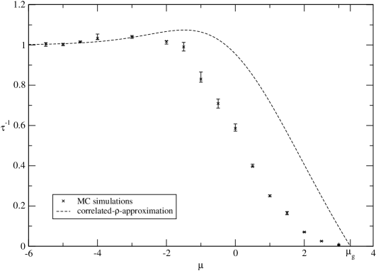
Figure 7: The inverse asymptotic relaxation time of $C(t)$ toward $C_{\text{li}}$ from numerical simulations (upper bounds) compared with the relaxation time from the correlated-$\rho$-approximation.

From the decay curves of $C(t)$ we can extract asymptotic relaxation times through a linearization of the function $f(t)=\ln(C(t)-C_{\text{li}})$ near $t\simeq T$. From the simulations we obtain $f(t)$ as a convex function, which means that the extracted relaxation times must be considered as lower bounds for the actual relaxation times. Results for the inverse asymptotic relaxation time $\tau^{-1}$ are shown in Fig. 7. The numerical data are plotted together with the result of the correlated-$\rho$-approximation, which follows directly from Eq. (48).

As mentioned before, the approximation correctly predicts a divergence of the equilibration time at $\mu_{g}\simeq 3.34$. The quantitative agreement is, however, poor when we approach the phase transition, only fare away numerical and approximate analytical data are close to each other. The figure indeed indicates that also the critical exponent of the equilibration-time divergence is different for the two cases. This suggests that the correlated $\rho$-approximation is still missing the asymptotically dominating slow process, i.e. a more detailed and well chosen set of order parameters is needed.

Decay of the autocorrelation function

In order to complete the picture, we show the decay curves of $C(t)$ for different $\mu$. The time axis has been shifted as to map $T/2\to 0$.

The left of Figs. 8 shows the curves for small $\mu$, i.e. far away from the spin-glass transition point. The qualitative and quantitative agreement between numerical and analytical data is quite satisfactory, even if the differences grow with larger values of the chemical potential. Note in particular that the approximation results are very good for short times, where by construction the equipartition assumption of PAS is valid, and for large times, where again by construction the assumption becomes correct. The largest deviation is found for intermediate times.

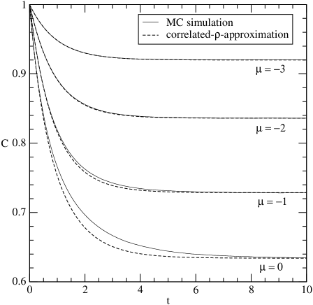
Figure 8: Decay curves of the autocorrelation function $C(t)$ for various $\mu$.

The right of the figures shows analogous curves for positive $\mu$. Since we are coming closer to the transition, the deviations show up more drastically, and the quantitative agreement for intermediate times becomes quite poor. Still, the initial part and the asymptotic value are reproduced correctly by the correlated-$\rho$-approximation.

VI Conclusion and outlook

In this paper, we have discussed the dynamical behaviour of a hard-sphere lattice-gas model on generalised Bethe lattices. The paper can be seen as a natural extension of the results presented in a preceding publication HaWe which was entirely dedicated to the study of equilibrium properties.

Since a technique allowing for an exact analysis of the non-equilibrium dynamics of finite-connectivity systems is still missing, we have applied a projective approximation scheme. Within this scheme, the dynamics is approximated by the time evolution of a finite number of global observables. Since the exact equations for their time evolution do not close, we have to use an approximate closure scheme. We have argued that the best and most natural closure scheme based only on the considered variables is the following: The true non-equilibrium state of the system is approximated by a pseudo-equilibrium distribution which is flat over all microscopic configurations being consistent with the values of all considered observables. The quality of this approximation depends crucially on the selection of the observable set: The latter has to include for sure a set of observables which are able to describe correctly the equilibrium state and to identify different thermodynamic phases. In general, a larger observable set gives also quantitatively better results, but the complexity of the underlying calculations increases considerably.

As a first application, we have studied the dynamics close to the liquid-crystal transition, both in the case of a second- and a first-order transition. Already the minimal description shows a very good qualitative and reasonable quantitative agreement with Monte-Carlo simulations, a more sophisticated level of approximation is hardly distinguishable from the numerical findings.

As a second application, we have also studied the dynamics close to the continuous spin-glass transition for the model on ordinary Bethe lattices. The chosen minimal approach is able to reproduce correctly the phase transition point, where the relaxation time diverges, but the quantitative agreement between numerical and analytical data for the dynamical behaviour close to the phase transition is quite poor. This signals that the selected observable set is not yet able to include the slowest relaxation process, and richer observable sets have to be used. We have in fact tried to do so, but the complexity of the resulting calculations was too large to arrive at a satisfactory result. Concerning the approximation scheme close to the spin glass transition, one probably should also go to observable sets which allow for the inclusion of explicitly replica symmetry breaking fluctuations. It may well be that the presented approach is able to reflect the longitudinal instability of the liquid solution within the replica-symmetric framework, and not the important replicon fluctuations breaking the replica symmetry MePaVi . Further research is necessary in this direction.

Another open question concerns the divergence of the equilibration time close to a discontinuous spin-glass transition as occurring on the generalised Bethe lattices. The latter is of fundamental interest in the context of the structural glass transition, but cannot be seen using PAS for the simple observable sets considered so far. This would also be of importance for the applicability of the method to kinetically constrained models RiSo ; SeBiTo , which have a trivial thermodynamics, but show a dynamical arrest due to kinetic constraints.

Acknowledgement: We are grateful to G. Semerjian and A. Zippelius for many interesting discussions. HHG acknowledges also the hospitality of the ISI Foundation in Turin, where parts of this research were worked out.

Appendix A Contributions to the changes in $\sigma_{j}$

We introduce the following functions of $j$:

$$P_{0}^{(0/1)}(j) = \begin{cases}\frac{\frac{k+1-j}{k+1}\,\sigma_{j}^{(0/1)}}{\sum_{l=0}^{k}\frac{k+1-l}{k+1}\,\sigma_{l}^{(0/1)}}\quad\text{for }j=0,\ldots,k\\ 0\quad\text{otherwise}\end{cases}$$ (50)

$$P_{1}^{(0/1)}(j) = \begin{cases}\frac{\frac{j+1}{k+1}\,\sigma_{j+1}^{(0/1)}}{\sum_{l=0}^{k}\frac{l+1}{k+1}\,\sigma_{l+1}^{(0/1)}}\quad\text{for }j=0,\ldots,k\\ 0\quad\text{otherwise}\end{cases}$$ (51)

$P_{0}^{(0/1)}(j)$ gives the probability that a 0/1-site, which is contained in an empty clique, has $j$ occupied neighbouring sites. $P_{1}^{(0/1)}(j)$ gives the probability that a 0/1-site, which is empty and which is contained in a clique that carries exactly one particle, has $j$ more occupied neighbouring sites (in other adjacent cliques). The values are exact in the $\Xi_{G}$-ensemble.

The actions of the dynamics are listed in the following together with their probabilities to occur:

ID	Action	Probability
$\mathcal{R}0$	Removal of a particle from the 0-lattice	$\frac{p}{p+1}\,\rho^{(0)}\,q_{0}$
$\mathcal{I}0$	Insertion of a particle to the 0-lattice	$\frac{p}{p+1}\,\sigma_{0}^{(0)}\,q_{1}$
$\mathcal{R}1$	Removal of a particle from the 1-lattice	$\frac{1}{p+1}\,\rho^{(1)}\,q_{0}$
$\mathcal{I}1$	Insertion of a particle to the 1-lattice	$\frac{1}{p+1}\,\sigma_{0}^{(1)}\,q_{1}$
$\mathcal{J}00$	Jump of a particle from a 0-site to a 0-site	$\frac{p}{p+1}\,\rho^{(0)}\,q_{s}\,\frac{p-1}{p}\,P_{1}^{(0)}(0)$
$\mathcal{J}01$	Jump of a particle from a 0-site to a 1-site	$\frac{p}{p+1}\,\rho^{(0)}\,q_{s}\,\frac{1}{p}\,P_{1}^{(1)}(0)$
$\mathcal{J}10$	Jump of a particle from a 1-site to a 0-site	$\frac{1}{p+1}\,\rho^{(1)}\,q_{s}\,P_{1}^{(0)}(0)$

The following table contains the contributions of the different actions of the dynamics to the changes in $\sigma_{j}^{(0/1)}$ or more precisely to the changes in the corresponding numbers of vacancies. The contributions are averages which are exact in the $\Xi_{G}$-ensemble apart from the exact $\delta$-contributions.

ID	Contribution to $\sigma_{j}^{(0)}$	Contribution to $\sigma_{j}^{(1)}$	Nature of the contribution
$\mathcal{R}0$	$+\,\delta_{0,j}$		direct
	$+\,(k+1)\,(p-1)\,P_{1}^{(0)}(j)$	$+\,(k+1)\,P_{1}^{(1)}(j)$	neighbours
	$-\,(k+1)\,(p-1)\,P_{1}^{(0)}(j-1)$	$-\,(k+1)\,P_{1}^{(1)}(j-1)$	neighbours
$\mathcal{I}0$	$-\,\delta_{0,j}$		direct
	$+\,(k+1)\,(p-1)\,P_{0}^{(0)}(j-1)$	$+\,(k+1)\,P_{0}^{(1)}(j-1)$	neighbours
	$-\,(k+1)\,(p-1)\,P_{0}^{(0)}(j)$	$-\,(k+1)\,P_{0}^{(1)}(j)$	neighbours
$\mathcal{R}1$		$+\,\delta_{0,j}$	direct
	$+\,(k+1)\,p\,P_{1}^{(0)}(j)$		neighbours
	$-\,(k+1)\,p\,P_{1}^{(0)}(j-1)$		neighbours
$\mathcal{I}1$		$-\,\delta_{0,j}$	direct
	$+\,(k+1)\,p\,P_{0}^{(0)}(j-1)$		neighbours
	$-\,(k+1)\,p\,P_{0}^{(0)}(j)$		neighbours
$\mathcal{J}00$	$+\,k\,(p-1)\,P_{1}^{(0)}(j)$	$+\,k\,P_{1}^{(1)}(j)$	backward
	$-\,k\,(p-1)\,P_{1}^{(0)}(j-1)$	$-\,k\,P_{1}^{(1)}(j-1)$	backward
	$+\,k\,(p-1)\,P_{0}^{(0)}(j-1)$	$+\,k\,P_{0}^{(1)}(j-1)$	forward
	$-\,k\,(p-1)\,P_{0}^{(0)}(j)$	$-\,k\,P_{0}^{(1)}(j)$	forward
$\mathcal{J}01$	$+\,\delta_{1,j}$	$-\,\delta_{1,j}$	intra-clique
	$+\,k\,(p-1)\,P_{1}^{(0)}(j)$	$+\,k\,P_{1}^{(1)}(j)$	backward
	$-\,k\,(p-1)\,P_{1}^{(0)}(j-1)$	$-\,k\,P_{1}^{(1)}(j-1)$	backward
	$+\,k\,p\,P_{0}^{(0)}(j-1)$		forward
	$-\,k\,p\,P_{0}^{(0)}(j)$		forward
$\mathcal{J}10$	$-\,\delta_{1,j}$	$+\,\delta_{1,j}$	intra-clique
	$+\,k\,p\,P_{1}^{(0)}(j)$		backward
	$-\,k\,p\,P_{1}^{(0)}(j-1)$		backward
	$+\,k\,(p-1)\,P_{0}^{(0)}(j-1)$	$+\,k\,P_{0}^{(1)}(j-1)$	forward
	$-\,k\,(p-1)\,P_{0}^{(0)}(j)$	$-\,k\,P_{0}^{(1)}(j)$	forward

The differential equations for the time-evolution of the observables $\sigma_{j}^{(0/1)}$ are obtained as follows. Let $N_{j}^{(0/1)}$ be the number of vacancies corresponding to $\sigma_{j}^{(0/1)}$. The average change of $N_{j}^{(0/1)}$ during the Monte-Carlo-time $\Delta t=1/N$ be $\Delta N_{j}^{(0/1)}$ which is obtained by choosing the contributions from the respective column in the above table, multiplying them with the probabilities for the corresponding actions of the dynamics and summing up the terms. The equations for $\Delta N_{j}^{(0/1)}$ become differential equations for $\sigma_{j}^{(0/1)}$ in the thermodynamic limit ($N\to\infty$) according to

$$\Delta N_{j}^{(0/1)}=\frac{N^{(0/1)}}{N}\>\frac{\Delta(N_{j}^{(0/1)}/N^{(0/1)})}{\Delta t}=\begin{cases}\>\frac{p}{p+1}\,\dot{\sigma}_{j}^{(0)}\\ \>\frac{1}{p+1}\,\dot{\sigma}_{j}^{(1)}\end{cases}$$ (52)

Here $N^{(0/1)}$ is the number of sites belonging to the respective sublattice.

References

- (1) P. Cheeseman, B. Kanefsky, and W.M. Taylor, in Proc. 13th Int. Joint Conf. Artif. Intell. (IJCAI-91), (eds. J. Mylopoulos and K. Reiter), 331 (Morgan Kaufmann, San Mateo, California, 1991).
- (2) D. Mitchell, B. Selman, and H. Levesque, in Proc. 10th Natl. Conf. on Artif. Intell. (AAAI-92), 440 (AAAI Press/MIT Press, Cambridge, Massachusetts, 1992).
- (3) B. Selman, S. Kirkpatrick, Science 264, 1297 (1994).
- (4) R. Monasson and R. Zecchina, Phys. Rev. Lett. 76, 3881 (1996).
- (5) R. Monasson, R. Zecchina, S. Kirkpatrick, B. Selman, L. Troyansky, Nature 400, 133 (1999).
- (6) M. Mezard, G. Parisi and R. Zecchina, Science 297, 812 (2002).
- (7) M. Weigt and A.K. Hartmann, Phys. Rev. Lett. 84, 6118 (2000).
- (8) R. Mulet, A. Pagnani, M. Weigt, and R. Zecchina, Phys. Rev. Lett. 89, 268701 (2002).
- (9) M. Mézard, G. Parisi and M.A. Virasoro, Spin Glass Theory and Beyond, (World Scientific, Singapore, 1987).
- (10) M. Mézard and G. Parisi, Eur. Phys. J. B 20, 217-233 (2001).
- (11) M. Mézard, G. Parisi, J. Stat. Phys. 111, 1 (2003).
- (12) S. Franz, M. Mézard, F. Ricci-Tersenghi, M. Weigt, R. Zecchina, Europhys. Lett. 55 (2001) 465.
- (13) G. Biroli and M. Mézard, Phys. Rev. Lett. 88, 025501 (2002).
- (14) M. Weigt and A.K. Hartmann, Europhys. Lett. 62, 533 (2003).
- (15) M. Pica Ciamarra, M. Tarzia, A. de Candia ans A. Coniglio, Phys. Rev. E 67, 057105 (2003).
- (16) O. Rivoire, G. Biroli, O.C. Martin and M. Mézard, Eur. Phys. J. B 37, 55-78 (2004).
- (17) H. Hansen-Goos and M. Weigt, J. Stat. Mech., P04006 (2005).
- (18) A. Barrat and R. Zecchina, Phys. Rev. E 59, R1299 (1999).
- (19) A. Montanari and F. Ricci-Tersenghi, Phys. Rev. Lett. 90, 017203 (2003).
- (20) G. Semerjian and L.F. Cugliandolo, Europhys. Lett. 61, 247 (2003).
- (21) G. Semerjian, L.F. Cugliandolo and A. Montanari, cond-mat/0304333, J. Stat. Phys. (to appear).
- (22) G. Semerjian and M. Weigt, J. Phys. A 37, 5525 (2004).
- (23) J.P.L. Hatchett et al., J. Phys. A 37, 6201 (2004).
- (24) G. Semerjian and R. Monasson, Phys. Rev. E 67, 066103 (2003).
- (25) W. Barthel, A.K. Hartmann, and M. Weigt, Phys. Rev. E 67, 066104 (2003).
- (26) A.C.C. Coolen and D. Sherrington, Phys. Rev. Lett. 71, 3886 (1993).
- (27) A.C.C. Coolen and D. Sherrington, J. Phys. A: Math. Gen. 27, 7687 (1994).
- (28) S. N. Laughton, A.C.C. Coolen and D. Sherrington, J. Phys. A: Math. Gen. 29, 763 (1996).
- (29) J.P.L. Hatchett, I. Perez Castillo, A.C.C. Coolen, and N.S. Skantzos, preprint cond-mat/0504313.
- (30) F. Ritort and P. Sollich, Adv. Phys. 52, 219 (2003).
- (31) M. Sellitto, G. Biroli, and C. Toninelli, Europhys. Lett. 69, 496 (2005).