Dephasing due to electron-electron interaction in a diffusive ring

Abstract

We study the effect of the electron-electron interaction on the weak localization correction of a ring pierced by a magnetic flux. We compute exactly the path integral giving the magnetoconductivity for an isolated ring. The results are interpreted in a time representation. This allows to characterize the nature of the phase coherence relaxation in the ring. The nature of the relaxation depends on the time regime (diffusive or ergodic) but also on the harmonics $n$ of the magnetoconductivity. Whereas phase coherence relaxation is non exponential for the harmonic $n=0$, it is always exponential for harmonics $n\neq 0$. Then we consider the case of a ring connected to reservoirs and discuss the effect of connecting wires. We recover the behaviour of the harmonics predicted recently by Ludwig & Mirlin [Phys. Rev. B69 (2004) 193306] for a large perimeter (compared to the Nyquist length). We also predict a new behaviour when the Nyquist length exceeds the perimeter.

I Introduction

In the classical description of transport in weakly disordered metals, elastic scattering by impurities leads to the finite Drude conductivity at low temperature. It is well-known that quantum interferences manifest themselves through a small sample dependent contribution, whose average, denoted by $\langle\Delta\sigma\rangle$, is called the weak localization correction. Dephasing strongly affects weak localization, which provides a powerful tool to probe phase coherence in disordered metals. The simplest approach to describe dephasing is to assume that the time dependence of the phase coherence relaxation is exponential. Such relaxation can be due for example to magnetic impurities HikLarNag80 . It is characterized by a time scale called the phase coherence time $\tau_{\varphi}$ and the weak localization correction to the conductivity takes the form

$$\langle\Delta\sigma\rangle=-2\frac{e^{2}D}{\pi}\int_{0}^{\infty}{\rm d}t\,{\cal P}(t)\,{\mbox{\large e}}^{-t/\tau_{\varphi}}\>,$$ (1)

where the so-called cooperon ${\cal P}(t)$ is the contribution to the return probability originating from quantum interferences between time reversed trajectories. It is solution of a diffusion equation. The factor $2$ stands for spin degeneracy and $D$ is the diffusion coefficient. We have set $\hbar=1$. In a quasi-one-dimensional infinite wire, the probability is well known to vary as ${\cal P}(t)=1/S\sqrt{4\pi Dt}$, where $S$ is the cross section of the wire, so that the weak localization correction has the familiar form

$$\langle\Delta\sigma\rangle=-\frac{e^{2}}{\pi S}L_{\varphi}$$ (2)

where $L_{\varphi}=\sqrt{D\tau_{\varphi}}$ is called the phase coherence length.

The measurement of the weak localization correction is possible thanks to its sensitivity to an external magnetic field. For a wire AltAro81 , the effect of a weak perpendicular magnetic field can be described by introducing an exponential reduction factor ${\mbox{\large e}}^{-t/\tau_{B}}$ in eq. (1), where the characteristic time is $\tau_{B}=3/(De^{2}B^{2}S)$ (for a wire of square cross section). Consequently the weak localization is given by eq. (2) with the addition of the inverse times, “à la Matthiesen” :

$$\langle\Delta\sigma\rangle=-\frac{e^{2}\sqrt{D}}{\pi S}\left(\frac{1}{\tau_{\varphi}}+\frac{1}{\tau_{B}}\right)^{-1/2}\>.$$ (3)

From the experimental point of view, this effect is of primary importance, since the magnetic field acts as a probe in order to study phase coherence and to extract $\tau_{\varphi}$ and its temperature dependence.

In the more complicated geometry of a ring, the field is also responsible for magnetoconductivity oscillations as predicted by Altshuler, Aronov & Spivak (AAS) AltAroSpi81 . The phase coherent return probability is sensitive to the flux $\phi$ through the ring. It has the simple harmonics expansion :

$${\cal P}(t)=\frac{1}{S\sqrt{4\pi Dt}}\sum_{n=-\infty}^{\infty}{\mbox{\large e}}^{-(nL)^{2}/4Dt}\,{\mbox{\large e}}^{{\rm i}n\theta}$$ (4)

where $\theta=4\pi\phi/\phi_{0}$ is the reduced flux ($\phi_{0}=h/e$ is the flux quantum). Each harmonic corresponds to a number of windings of the diffusive trajectories around the ring. The relation (1), with (4), immediately leads to the familiar result of AAS for the weak localization correction to the average conductivity in a ring :

$$\langle\Delta\sigma(\theta)\rangle=-\frac{e^{2}}{\pi S}\,L_{\varphi}\,\frac{\sinh(L/L_{\varphi})}{\cosh(L/L_{\varphi})-\cos\theta}\>.$$ (5)

The harmonics of this $\phi_{0}/2$-periodic correction decay exponentially with the perimeter $L$ of the ring :

$$\langle\Delta\sigma_{n}\rangle=\int_{0}^{2\pi}\frac{{\rm d}\theta}{2\pi}\,\langle\Delta\sigma(\theta)\rangle\,{\mbox{\large e}}^{-{\rm i}n\theta}=-\frac{e^{2}}{\pi S}\,L_{\varphi}\,{\mbox{\large e}}^{-|n|L/L_{\varphi}}.$$ (6)

The combination of the two effects of the magnetic field, AAS oscillations and penetration in the wires, is obtained by perfoming the substitution : $1/\tau_{\varphi}\rightarrow 1/\tau_{\varphi}+1/\tau_{B}$ in eq. (5).

Despite the exponential damping in eq. (1) describes correctly several dephasing mechanisms like spin-orbit scattering and spin-flip HikLarNag80 , or the effect of an external magnetic field AltAro81 , a precise description of the electron-electron interaction requires a more elaborate treatment. In a pioneering paper, Altshuler, Aronov & Khmelnitskii (AAK) AltAroKhm82 ; AltAro85 have shown that the dephasing due to the electron-electron interaction can be described in a one-particle picture by coupling the electron to a fluctuating classical electromagnetic field. They obtained a result which can be cast in the form

$$\langle\Delta\sigma\rangle=-2\frac{e^{2}D}{\pi}\int_{0}^{\infty}{\rm d}t\,{\cal P}(t)\,f(t/\tau_{N})\,{\mbox{\large e}}^{-t/\tau_{\varphi}}\>,$$ (7)

where $f(x)$ is a decreasing dimensionless function. We have also incorporated an exponential relaxation (if it is due to the external magnetic field $B$ we have simply $\tau_{\varphi}\to\tau_{B}$). The characteristic time, called the Nyquist time, is given by footnote1

$$\tau_{N}=\left(\frac{\hbar^{2}\sigma_{0}S}{e^{2}k_{B}T\sqrt{D}}\right)^{2/3}\>,$$ (8)

where $T$ is the temperature and $k_{B}$ the Boltzmann’s constant (in the following we will set $\hbar=k_{B}=1$). $\sigma_{0}=2e^{2}\rho_{0}D$ is the Drude conductivity and $\rho_{0}$ the density of states at Fermi energy, per spin channel. The $T^{-2/3}$ power law has been observed in a variety of experiments (see for example refs. EchGerBozBogNil93b ; GouPiePotEstBir00 ) and is the signature of the electron-electron interaction in quasi-1d wires. In the case of an infinite wire, AAK found that the weak localization correction is given by AltAroKhm82 ; footnote1

$$\langle\Delta\sigma\rangle=\frac{e^{2}}{\pi S}L_{N}\,\frac{{\rm Ai}(\tau_{N}/\tau_{\varphi})}{{\rm Ai}^{\prime}(\tau_{N}/\tau_{\varphi})}\>,$$ (9)

where ${\rm Ai}(z)$ is the Airy function and ${\rm Ai}^{\prime}(z)$ its derivative. We have introduced the Nyquist length $L_{N}=\sqrt{D\tau_{N}}$ which characterizes the scale over which the electron-electron interaction is effective. It can be conveniently rewritten as :

$$L_{N}=\left(\frac{\sigma_{0}SD}{e^{2}T}\right)^{1/3}=\left(\frac{\alpha_{d}}{\pi}N_{c}\ell_{e}L_{T}^{2}\right)^{1/3}\>,$$ (10)

where we have introduced the thermal length $L_{T}=\sqrt{D/T}$, the number of channels $N_{c}$, the elastic mean free path $\ell_{e}$ and a numerical factor $\alpha_{d}$ that depends on the dimension $d$ ($\alpha_{1}=2$, $\alpha_{2}=\pi/2$ and $\alpha_{3}=4/3$) AkkMon04 ; TexMon04 ; TexMonAkk05 . We have expressed the Drude conductivity as $\sigma_{0}=2\frac{e^{2}}{h}{\alpha_{d}N_{c}\ell_{e}}/{S}$ (the factor 2 stands for spin degeneracy).

In addition to the prediction of the power law $\tau_{N}\propto T^{-2/3}$ for the coherence time, an important outcome of the AAK theory is that the result (9) obviously breaks the addition rule of inverse times. This indicates that the phase relaxation characterized by the function $f(t/\tau_{N})$ is indeed non exponential. This function has been calculated recently in ref. MonAkk05 where it was found that it varies as footnote2 ${\mbox{\large e}}^{-(\sqrt{\pi}/4)(t/\tau_{N})^{3/2}}$ for $t\lesssim\tau_{N}$. However the study of the function $f(t/\tau_{N})$ shows that it is very close to an exponential ${\mbox{\large e}}^{-t/2\tau_{N}}$ and eq. (9) only deviates from $\langle\Delta\sigma\rangle=-\frac{e^{2}\sqrt{D}}{\pi S}(\frac{1}{2\tau_{N}}+\frac{1}{\tau_{\varphi}})^{-1/2}$, that is eq. (3), by no more than $4\%$ PieGouAntPotEstBir03 ; AkkMon04 ; MonAkk05 . This explains why it is very difficult to observe experimentally the functional form (9) and most of the magnetoconductance measurements in wires have been analyzed assuming the form (3).

In the paper of AAK, only simple geometries (like wire and plane) were considered and it is not clear how the non exponential relaxation of phase coherence affects the weak localization for a nontrivial geometry. In a recent paper, Ludwig & Mirlin (LM) LudMir04 have addressed the question of dephasing due to the electron-electron interaction in a ring. The dephasing is then probed by the harmonics of the magnetoconductance oscillations. These authors found that these harmonics decay with the perimeter $L$ of the ring in an unexpected way. LM’s result can be cast in the form footnote3

$$\langle\Delta\sigma_{n}\rangle\propto{\mbox{\large e}}^{-|n|(L/L_{N})^{3/2}}\>.$$ (11)

This result is quite interesting, because this nontrivial non exponential decay of the harmonics leads to an unexpected ${\mbox{\large e}}^{-nL^{3/2}T^{1/2}}$ temperature behaviour, instead of the incorrect behaviour ${\mbox{\large e}}^{-nL/L_{N}}={\mbox{\large e}}^{-nLT^{1/3}}$ naively expected from a simple substitution $\tau_{\varphi}\to\tau_{N}$ in the AAS harmonics (6). It also shows that the geometry of the system may play an important role in the nature of the dephasing mechanism.

The work of LM was mainly devoted to the study of Aharonov-Bohm (AB) oscillations in a single ring. The study of AB amplitude, rather than AAS, is motivated by the lack of disorder averaging in this case. The amplitude of AB oscillations is given by the harmonics $\langle\delta\sigma_{n}^{2}\rangle$ of the conductivity correlation function $\langle\delta\sigma(B)\,\delta\sigma(B^{\prime})\rangle$. As pointed out by LM, these harmonics are expected to be directly related to the AAS harmonics by the following relation

$$\langle\delta\sigma_{n}^{2}\rangle\sim\frac{L_{T}^{2}}{L}\langle\Delta\sigma_{n}\rangle\>,$$ (12)

where $L_{T}=\sqrt{D/T}$ is the thermal length. This expression extends the result of Aleiner & Blanter AleBla02 who studied the relation between conductance fluctuations and weak localization in a wire and a plane when dephasing is due to the electron-electron interaction. An important consequence of this relation is that the effect of dephasing on weak localization and conductance fluctuations is governed by the same length scale $L_{N}$. We re-examine this relation and give a more general proof in appendix E.

In our paper, we reconsider the question of weak localization in a ring in the presence of electron-electron interaction. Our main goal is to provide a physical picture as well as a detailed understanding of the results obtained by LM LudMir04 . The physical reason for the geometry dependence of the dephasing can be understood in the following heuristic way. For a pair of time reversed trajectories, we denote by $\Phi$ the random phase brought by the fluctuating electromagnetic field. Average over the Gaussian fluctuations of the field is denoted by $\langle\cdots\rangle_{V}$. Averaging the phase $\langle{\mbox{\large e}}^{{\rm i}\Phi}\rangle_{V}$ produces an exponential damping ${\mbox{\large e}}^{-\frac{1}{2}\langle\Phi^{2}\rangle_{V}}$ responsible for phase coherence relaxation (this exponential is related to the function $f(t/\tau_{N})$ in eq. (7)). For a quasi-1d system, the typical damping rate associated to a diffusive trajectory can be written in the form

$$\frac{{\rm d}\langle\Phi^{2}\rangle_{V}}{{\rm d}t}\sim\frac{e^{2}T}{\sigma_{0}S}\,r(t)=\frac{1}{\tau_{N}}\frac{r(t)}{\sqrt{D\tau_{N}}}\>,$$ (13)

where $r(t)$ designates the typical distance explored by the diffusive trajectory over a time scale $t$. As pointed out in ref. Fer04 , eq. (13) can be understood as a local form of the Johnson-Nyquist theorem : since the phase and the potential are related by $\dot{\Phi}=V$, eq. (13) measures the potential fluctuations $\frac{{\rm d}}{{\rm d}{t}}\langle\Phi^{2}\rangle_{V}=\int{\rm d}{t}\langle V(t)V(0)\rangle_{V}=2e^{2}TR_{t}$, where $R_{t}\sim{r(t)/(S\sigma_{0})}$ is the resistance of a wire of length $r(t)$. It is clear from eq. (13) that the dephasing depends on the nature of the diffusive trajectories. Two regimes can be distinguished :

• The diffusive regime.– In this regime, the boundaries of the system play no role and the diffusion follows the behaviour obtained in an infinite wire, therefore $r(t)\sim\sqrt{Dt}$, so that

  $$\langle\Phi^{2}\rangle_{V}\propto\left(\frac{t}{\tau_{N}}\right)^{3/2}\>.$$ (14)

  Therefore we expect the phase relaxation to be non exponential $f(t/\tau_{N})\sim\exp{-(t/\tau_{N})^{3/2}}$.

• The ergodic regime.– In this case, the diffusive trajectories explore the whole system. This corresponds to time scales larger than the Thouless time $\tau_{D}=L^{2}/D$. The characteristic length is given by the size of the system (the ring) $r(t)\sim L$ and

  $$\langle\Phi^{2}\rangle_{V}\propto\frac{\sqrt{\tau_{D}}}{\tau_{N}^{3/2}}\,t=\frac{t}{\tau_{c}}\>.$$ (15)

  We expect the phase relaxation to be exponential, $\exp{-t/\tau_{c}}$ , where the time scale

  $$\tau_{c}=\frac{\sigma_{0}S}{e^{2}TL}=\frac{\tau_{N}^{3/2}}{\tau_{D}^{1/2}}$$ (16)

  is size dependent and is a nontrivial combination of the Thouless time and the Nyquist time.

It is clear that the function $f(t/\tau_{N})$ in eq. (7) must be replaced by a more complicated function $f(t/\tau_{N},t/\tau_{D})$ to account for finite size effect and describe both regimes. We expect that the winding around the ring plays an important role and a dephasing of different nature for trajectories which enclose the ring (corresponding to the $n\neq 0$ harmonics of the flux dependence) and for trajectories which do not encircle the ring (corresponding to the $n=0$ harmonic). For harmonics $n\neq 0$, the trajectories necessarily explore the whole ring and the phase coherence relaxation is always exponential. This is the origin for the new behaviour found by LM. For the harmonic $n=0$ we can distinguish two different regimes corresponding to non exponential and exponential relaxation. In other terms, the function $f(t/\tau_{N},t/\tau_{D})$ depends also on the winding number $n$.

In order to give a firm basis to these arguments, we have reconsidered the calculation of LM. These authors have studied a symmetric ring connected by two arms to reservoirs and have derived the weak localization correction within an instanton approximation for the functional integral describing the effect of the fluctuating field. The instanton approach is only valid in the limit of large perimeter of the ring (compared to the length scale characterizing the electron-electron interaction), that is when $L\gg L_{N}$ (i.e. $\tau_{D}\gg\tau_{N}$).

In our work we have followed a different strategy. We first consider the case of an isolated ring for which it is possible to compute exactly the path integral for any value of $L/L_{N}$. This path integral formulation is introduced in section II, and the exact solution is given in section III, where a closed expression for the harmonics of the magnetoconductivity is provided and analyzed in several regimes.

Our result agrees with the exponential behaviour (11) found by LM. However we will point out that LM estimated an incorrect prefactor (leading to an incorrect temperature dependence). LM’s result can be written as $\langle\Delta\sigma_{n}\rangle_{\rm LM}\sim L_{N}^{9/4}{\mbox{\large e}}^{-|n|(L/L_{N})^{3/2}}$ whereas we will show that the correct result is $\langle\Delta\sigma_{n}\rangle\sim{L_{N}}{\mbox{\large e}}^{-|n|(L/L_{N})^{3/2}}$. Note that it could seem at first sight that the difference comes from the fact that our exact solution stands for an isolated ring whereas LM considered a connected ring, however we will see that the two situations are closely related. Moreover the isolated ring leads to consider a path integral exactly similar to the one studied by LM which allows us to trace back to the origin of LM’s incorrect prefactor (we have also estimated in appendix C the path integral within the instanton approach used by LM. We treat carefully the prefactor within this approach).

Our exact solution takes also into account the effect of an exponential relaxation of phase coherence ($\tau_{\varphi}$). We will show that both kinds of dephasing mechanisms (i.e. $\tau_{N}$ and $\tau_{\varphi}$) combine in a nontrivial way.

In section IV we analyze the exact result in a time representation, that is we study the function $f(t/\tau_{N},t/\tau_{D})$ that generalizes the $f(t/\tau_{N})$ of eq. (7). A special emphasis is put on the difference between harmonics $n=0$ and $n\neq 0$ : although the phase coherence relaxation for the harmonic $n=0$ is either non exponential (at short times) or exponential (at large times), it is always exponential for harmonics $n\neq 0$. This analysis in time representation is used in the section V where we discuss the effect of connecting wires : in a transport experiment, the ring is necessary connected to wires that can strongly affect the magnetoconductance. This has been discussed recently for the case of exponential relaxation of phase coherence TexMon05 . Although we do not expect a strong effect of the connecting wires on the harmonics in the regime $L\gg L_{N}$, we will show by some simple arguments that the behaviour (11) is strongly modified in the other regime $L\ll L_{N}$.

II Path integral formulation

We recall the basic ideas of AAK’s approach AltAroKhm82 . In dimension $d\leqslant 2$ the dephasing is dominated by small energy transfers. The dephasing for one electron can be modeled through the coupling of the electron with a classical fluctuating electric potential $V(r,t)$, whose fluctuations are given by the fluctuation-dissipation theorem. In a Fourier representation, the correlations are given by $\langle\tilde{V}\,\tilde{V}\rangle_{(\vec{q},\omega)}=\frac{2e^{2}T}{\sigma_{0}q^{2}}$. In a time-space representation it reads

$$\left\langle V(\vec{r},t)\,V(\vec{r}\,^{\prime},t^{\prime})\right\rangle_{V}=\frac{2e^{2}}{\sigma_{0}}T\,\delta(t-t^{\prime})\,P_{d}(\vec{r},\vec{r}\,^{\prime})\>,$$ (17)

where $\left\langle\cdots\right\rangle_{V}$ designates averaging over the Gaussian fluctuations of the potential. $P_{d}(\vec{r},\vec{r}\,^{\prime})$ is the diffuson, solution of the equation $-\Delta P_{d}(\vec{r},\vec{r}\,^{\prime})=\delta(\vec{r}-\vec{r}\,^{\prime})$ (it is understood that the zero mode diverging contribution is not taken into account in the diffuson of eq. (17). This point is discussed in appendix A). Eq. (17) clearly exhibits the long range nature of the spatial correlations.

The description of AAK allows to perform a mean-field-like but non-perturbative treatment of the electron-electron interaction. We denote by $\widetilde{\cal P}$ the cooperon that includes the effect of the electron-electron interaction. It can be conveniently written with a path integration over the diffusive trajectories of the electron

$$\widetilde{\cal P}(\vec{r},\vec{r};t)=\left\langle\int_{\vec{r}(0)=\vec{r}}^{\vec{r}(t)=\vec{r}}{\cal D}\vec{r}(\tau)\,{\mbox{\large e}}^{-\int_{0}^{t}{\rm d}\tau\,\frac{\dot{\vec{r}}(\tau)^{2}}{4D}\ +\ {\rm i}\Phi[\vec{r}(\tau)]}\right\rangle_{V}$$ (18)

where the phase

$$\Phi[\vec{r}(\tau)]=\int_{0}^{t}{\rm d}\tau\,\left[V(\vec{r}(\tau),\tau)-V(\vec{r}(\tau),\bar{\tau})\right]\>,$$ (19)

with $\bar{\tau}=t-\tau$, is the phase difference between the two time reversed trajectories. In the presence of a static magnetic field, a coupling $2{\rm i}{e}\int_{0}^{t}{\rm d}\tau\,\dot{\vec{r}}(\tau)\cdot\vec{A}(\vec{r}(\tau))$ to the vector potential $\vec{A}(\vec{r})$ must be added in the action. In a ring of perimeter $L$ pierced by a magnetic flux $\phi$, we have $2eA=\theta/L$, where $\theta=4\pi\phi/\phi_{0}$ is the reduced flux.

The cooperon has the structure $\widetilde{\cal P}(\vec{r},\vec{r};t)={\cal P}(\vec{r},\vec{r};t)\,\langle{\mbox{\large e}}^{{\rm i}\Phi}\rangle_{V,{\cal C}}$ where ${\cal P}(\vec{r},\vec{r};t)$ is the cooperon in the absence of the electron-electron interaction and $\langle\cdots\rangle_{{\cal C}}$ denotes averaging over closed Brownian curves.

The average over the Gaussian fluctuations of the field in (18) can be performed thanks to the relation $\langle{\mbox{\large e}}^{{\rm i}\Phi}\rangle_{V}={\mbox{\large e}}^{-\frac{1}{2}\langle\Phi^{2}\rangle_{V}}$. The term that appears in the action is

$$\frac{1}{2}\langle\Phi^{2}\rangle_{V}=\frac{2e^{2}T}{\sigma_{0}}\int_{0}^{t}{\rm d}\tau\,W(\vec{r}(\tau),\vec{r}(\bar{\tau}))$$ (20)

where we have introduced the function $W$, defined in the most symmetric way by :

$$W(\vec{r},\vec{r}\,^{\prime})=\frac{P_{d}(\vec{r},\vec{r})+P_{d}(\vec{r}\,^{\prime},\vec{r}\,^{\prime})}{2}-P_{d}(\vec{r},\vec{r}\,^{\prime})\>.$$ (21)

For one-dimensional wires of section $S$ we have $P_{d}(\vec{r},\vec{r}\,^{\prime})\to\frac{1}{S}P_{d}(x,x^{\prime})$, where $P_{d}(x,x^{\prime})$ is now the one dimensional diffuson. Similar subsitutions holds for $W$ and $\widetilde{\cal P}$. The cooperon finally reads

$$\widetilde{\cal P}(x,x;t) = \int_{x(0)=x}^{x(t)=x}{\cal D}x(\tau)\,$$

$$\times{\mbox{\large e}}^{-\int_{0}^{t}{\rm d}\tau\,\Big{[}\frac{\dot{x}(\tau)^{2}}{4D}+\frac{2}{\sqrt{D}\tau_{N}^{3/2}}\,W(x(\tau),x(\bar{\tau}))\Big{]}}\>,$$

where we have used the definition of the Nyquist time (8). The weak localization correction is now given by

$$\langle\Delta\sigma\rangle=-2\frac{e^{2}D}{\pi S}\int_{0}^{\infty}{\rm d}t\,\widetilde{\cal P}(x,x;t)\,{\mbox{\large e}}^{-t/\tau_{\varphi}}\>,$$ (23)

which is another way to write eq. (7) (note that for a translation device such as a wire or a ring, $\widetilde{\cal P}(x,x;t)$ is independent on $x$).

Scaling.– If we introduce the dimensionless variables $u=\tau/t$ and $y=x/\sqrt{Dt}$, using the expression of $W(x,x^{\prime})$ given below by eq. (27), we get, for a ring or for a finite connected wire :

$$\widetilde{\cal P}(x,x;t)=\frac{1}{\sqrt{Dt}}\int_{y(0)=y}^{y(1)=y}{\cal D}y(u)\,$$ (24)

$${\mbox{\large e}}^{-\int_{0}^{1}{\rm d}u\,\Big{[}\frac{1}{4}\dot{y}(u)^{2}+2(\frac{t}{\tau_{N}})^{3/2}|y(u)-y(\bar{u})|\left(1-(\frac{t}{\tau_{D}})^{1/2}|y(u)-y(\bar{u})|\right)\Big{]}}\>,$$

where $\bar{u}=1-u$. We obtain the structure assumed in the introduction :

$$\widetilde{\cal P}(x,x;t)={\cal P}(x,x;t)\times f\!\left(\frac{t}{\tau_{N}},\frac{t}{\tau_{D}}\right)\>,$$ (25)

where $f(x,y)$ is a dimensionless function. Finally it is clear that the integration over time, eq. (23), leads to a conductivity of the form

$$\langle\Delta\sigma\rangle=\frac{e^{2}}{S}L\times g\!\left(\frac{L}{L_{N}},\frac{L}{L_{\varphi}}\right)\>,$$ (26)

where $g(x,y)$ is a dimensionless function.

In the following we will omit the section of the wire.

How to get rid of time-nonlocality ?– The expressions (18,II) were the starting point of ref. AltAroKhm82 in which the correction was computed in the case of an infinite plane and an infinite wire. A first difficulty to evaluate the path integral (II) is the nonlocality in time of the action. This problem can be overcome thanks to the translation invariance which makes the function $W(x,x^{\prime})$ a function of the difference $x-x^{\prime}$ only. Such a property is true only in few cases. More precisely, for the infinite wire (AAK) and a finite isolated wire, the function is given by $W(x,x^{\prime})=\frac{1}{2}|x-x^{\prime}|$. For the connected wire and the isolated ring, it reads (see appendix A)

$$W(x,x^{\prime})=\frac{1}{2}|x-x^{\prime}|\left(1-\frac{|x-x^{\prime}|}{L}\right)\>.$$ (27)

For a translation invariant problem we can follow the strategy of AAK : separate the path integral into two parts over the time intervals $[0,t/2]$ and $[t/2,t]$ with $\int_{x,0}^{x,t}{\cal D}x(\tau)\rightarrow\int{\rm d}x^{\prime}\int_{x^{\prime},t/2}^{x,t}{\cal D}x_{1}(\tau)\int_{x,0}^{x^{\prime},t/2}{\cal D}x_{2}(\tau)$, then perform the change of variables $R(\tau)=\frac{x_{1}(\tau)+x_{2}(\bar{\tau})}{\sqrt{2}}$ and $\rho(\tau)=\frac{x_{1}(\tau)-x_{2}(\bar{\tau})}{\sqrt{2}}$ (the Jacobian is 1). Since $W(x,x^{\prime})$ is only function of $x-x^{\prime}$, the action possesses a potential term $W(x_{1}(\tau),x_{2}(\bar{\tau}))=W(\rho(\tau),0)$ function of $\rho$ only, therefore local in time.

This result is actually due to a general property mentioned in ref. ComDesTex05 . The path integral (II) extends over all Brownian paths coming back to their initial value (these paths are called Brownian bridges). If we consider a Brownian bridge $(x(\tau),0\leqslant\tau\leqslant t\,|\,x(0)=x(t)=0)$ we can write the following equality in law :

$$x(\tau)-x(t-\tau)\stackrel{{\scriptstyle\mbox{\tiny\rm(law)}}}{{=}}x(2\tau)\hskip 7.11317pt\mbox{ for }\tau\in[0,t/2]\>.$$ (28)

(Two random variables distributed according to the same probability distribution are said to be “equal in law”). Therefore it follows that $\int_{0}^{t}{\rm d}\tau\,{\cal V}(x(\tau)-x(\bar{\tau}))\stackrel{{\scriptstyle\mbox{\tiny\rm(law)}}}{{=}}\int_{0}^{t}{\rm d}\tau\,{\cal V}(x(\tau))$ for any function ${\cal V}(x)$. This immediately gives

$$\int_{x(0)=x}^{x(t)=x}{\cal D}x(\tau)\,{\mbox{\large e}}^{-\int_{0}^{t}{\rm d}\tau\,\left[\frac{\dot{x}(\tau)^{2}}{4D}+{\cal V}(x(\tau)-x(\bar{\tau}))\right]}$$

$$=\int_{x(0)=0}^{x(t)=0}{\cal D}x(\tau)\,{\mbox{\large e}}^{-\int_{0}^{t}{\rm d}\tau\,\left[\frac{\dot{x}(\tau)^{2}}{4D}+{\cal V}(x(\tau))\right]}\>.$$ (29)

III Exact calculation of the path integral in the isolated ring

From eqs. (II,II) we can write the weak localization in the form :

$$\langle\Delta\sigma\rangle = -2\frac{e^{2}}{\pi}\int_{0}^{\infty}{\rm d}t\,{\mbox{\large e}}^{-t/L_{\varphi}^{2}}\int_{x(0)=0}^{x(t)=0}{\cal D}x(\tau)\,$$ (31)

$$\times{\mbox{\large e}}^{\int_{0}^{t}{\rm d}\tau\,\left[-\frac{\dot{x}^{2}}{4}+2{\rm i}e\dot{x}\,A(x)-\frac{2}{L_{N}^{3}}\,W(x(\tau),0)\right]}$$

$$=-\frac{2e^{2}}{\pi}\>\langle\kern 1.29167ptx=0\kern 1.29167pt|\frac{1}{\frac{1}{L_{\varphi}^{2}}-{\rm D}_{x}^{2}+\frac{1}{L_{N}^{3}}\left(|x|-\frac{1}{L}x^{2}\right)}|\kern 1.29167ptx=0\kern 1.29167pt\rangle$$

where we have rescaled the time to get rid of the diffusion constant, and introduced the coupling to the magnetic field. Inside the ring the vector potential is given by $2eA(x)=\theta/L$, therefore the covariant derivative is ${\rm D}_{x}={\rm d}/{\rm d}{x}-{\rm i}\theta/L$.

III.1 The result for $L_{\varphi}=\infty$

As we have mentioned in the introduction, the most striking effect of the electron-electron interaction is a modification of the dependence of the AAS oscillations as a function of $L/L_{N}$. For this reason we begin this section by emphasizing the results for two limiting cases demonstrated below.

$\bullet$ Small perimeter $L\ll L_{N}$. In this case :

$$\langle\Delta\sigma_{n}\rangle\simeq-\frac{e^{2}}{\pi}\,{L}\,\sqrt{6}\left(\frac{L_{N}}{L}\right)^{3/2}{\mbox{\large e}}^{-|n|\frac{1}{\sqrt{6}}(\frac{L}{L_{N}})^{3/2}}\>.$$ (32)

$\bullet$ Large perimeter $L\gg L_{N}$. This regime is the one studied by LM LudMir04 ; footnote3 . We obtain

$$\langle\Delta\sigma_{n}\rangle\simeq\frac{e^{2}}{\pi}\,{L_{N}}\,\frac{{\rm Ai}(0)}{{\rm Ai}^{\prime}(0)}\>\left(\frac{\sqrt{3}}{2}\right)^{|n|}{\mbox{\large e}}^{-|n|\frac{\pi}{8}(\frac{L}{L_{N}})^{3/2}}\>,$$ (33)

where $\frac{{\rm Ai}(0)}{{\rm Ai}^{\prime}(0)}=-\frac{\Gamma(1/3)}{3^{1/3}\Gamma(2/3)}\simeq-1.372$. The exponential behaviour coincides exactly with the one obtained by LM (see footnote1 ). However our prefactor differs as will be discussed in section V.

III.2 Computation of the cooperon

Starting from eq. (31) we introduce the rescaled variable $\chi=x/L$. Then the weak localization correction rewrites

$$\langle\Delta\sigma\rangle=-2\frac{e^{2}}{\pi}{L}\>C(0,0)\>,$$ (34)

where the Green’s function is solution of

$$\left[-\left(\frac{{\rm d}}{{\rm d}\chi}-{\rm i}\theta\right)^{2}+\frac{L^{3}}{L_{N}^{3}}\left(|\chi|-\chi^{2}\right)+\frac{L^{2}}{L_{\varphi}^{2}}\right]C(\chi,\chi^{\prime})$$

$$=\delta(\chi-\chi^{\prime})$$ (35)

for $\chi\in[0,1]$ and periodic boundary conditions. We introduce the notation

$$a=\left(\frac{L}{L_{N}}\right)^{3}\hskip 7.11317pt\mbox{ and }\hskip 7.11317ptb=\left(\frac{L}{L_{\varphi}}\right)^{2}\>.$$ (36)

We first consider the Cauchy problem. The differential equation

$$\left[-\frac{{\rm d}^{2}}{{\rm d}\chi^{2}}+a\,\chi(1-\chi)+b\right]f(\chi)=0$$ (37)

is a hypergeometric equation and can be solved by standard methods NikOuv83 which suggest the following transformation $f(\chi)={\mbox{\large e}}^{-\frac{1}{2}s^{2}}\,y(s)$, where the variable is

$$s={\mbox{\large e}}^{{\rm i}\frac{\pi}{4}}a^{1/4}\left(\chi-\frac{1}{2}\right)\>.$$ (38)

It is now easy to see that the function $y(s)$ is solution of the Hermite equation. A solution of (37) is

$$\tilde{f}(\chi)={\mbox{\large e}}^{-\frac{1}{2}s^{2}}\,H_{\nu}(s)\>,$$ (39)

where $H_{\nu}(s)$ is the Hermite function (see appendix B). The index $\nu$ reads

$$\nu=-\frac{1}{2}+{\rm i}\omega\hskip 14.22636pt\mbox{with}\hskip 14.22636pt\omega=\frac{\sqrt{a}}{8}+\frac{b}{2\sqrt{a}}\>.$$ (40)

Thanks to the symmetry of the differential equation with respect to the substitution $\chi\leftrightarrow 1-\chi$, and since $\tilde{f}(\chi)$ is not invariant under this transformation, another possible solution is $\tilde{f}(1-\chi)={\mbox{\large e}}^{-\frac{1}{2}s^{2}}\,H_{\nu}(-s)$.

In order to construct the Green’s function $C(\chi,\chi^{\prime})$ we introduce another solution of eq. (37) satisfying the boundary conditions

$$f(0)=1\hskip 7.11317pt\mbox{and}\hskip 7.11317ptf(1)=0\>.$$ (41)

This solution is related to $\tilde{f}(\chi)$ by

$$f(\chi)=\frac{\tilde{f}(0)\tilde{f}(\chi)-\tilde{f}(1)\tilde{f}(1-\chi)}{\tilde{f}(0)^{2}-\tilde{f}(1)^{2}}\>.$$ (42)

The derivatives of $f(\chi)$ at $\chi=0$ and $1$ will be central quantities in the following. They can be related to the derivatives of $\tilde{f}(\chi)$ as

$$f^{\prime}(0) = \frac{\tilde{f}(0)\tilde{f}^{\prime}(0)+\tilde{f}(1)\tilde{f}^{\prime}(1)}{\tilde{f}(0)^{2}-\tilde{f}(1)^{2}}$$ (43)

$$f^{\prime}(1) = \frac{\tilde{f}(0)\tilde{f}^{\prime}(1)+\tilde{f}(1)\tilde{f}^{\prime}(0)}{\tilde{f}(0)^{2}-\tilde{f}(1)^{2}}\>.$$ (44)

Then the cooperon is given by Des00 ; TexMonAkk05  :

$$C(\chi,\chi^{\prime}) = \frac{{\mbox{\large e}}^{{\rm i}\theta(\chi-\chi^{\prime})}}{{\cal M}}\Big{[}f(\chi)\,f(\chi^{\prime})+{\mbox{\large e}}^{{\rm i}\theta}\,f(\chi)\,f(1-\chi^{\prime})$$ (45)

$$+{\mbox{\large e}}^{-{\rm i}\theta}\,f(1-\chi)\,f(\chi^{\prime})+f(1-\chi)\,f(1-\chi^{\prime})\Big{]}$$

$$-\frac{{\mbox{\large e}}^{{\rm i}\theta(\chi-\chi^{\prime})}}{f^{\prime}(1)}f(\mathop{\mathrm{max}}\nolimits\left(\chi,\chi^{\prime}\right))\,f(1-\mathop{\mathrm{min}}\nolimits\left(\chi,\chi^{\prime}\right))\>,$$

where ${\cal M}=-2f^{\prime}(0)+2\cos\theta\,f^{\prime}(1)$. At the origin we obtain $C(0,0)=\frac{1}{{\cal M}}$, therefore

$$\langle\Delta\sigma\rangle=-\frac{e^{2}}{\pi}{L}\>\frac{1}{-f^{\prime}(0)+f^{\prime}(1)\,\cos\theta}\>.$$ (46)

This result shows that in the most general case with exponential relaxation ($\tau_{\varphi}$) and electron-electron interaction ($\tau_{N}$), the flux dependence of the weak localization correction has still the same structure as AAS, eq. (5). As a consequence the harmonics still decay exponentially with $n$ :

$$\langle\Delta\sigma_{n}\rangle = -\frac{e^{2}}{\pi}{L}\>\frac{{\mbox{\large e}}^{-|n|\ell_{\rm eff}}}{\sqrt{f^{\prime}(0)^{2}-f^{\prime}(1)^{2}}}\>,$$ (47)

where, by analogy with eq. (6), we have introduced an effective “perimeter” $\ell_{\rm eff}$, defined by

$$\cosh\ell_{\rm eff}=\frac{f^{\prime}(0)}{f^{\prime}(1)}\>.$$ (48)

The equations (47,48) are central results of the paper. We now analyze several limiting cases, which requires a detailed study of $\tilde{f}(0)$, $\tilde{f}^{\prime}(0)$, $\tilde{f}(1)$ and $\tilde{f}^{\prime}(1)$.

III.3 No electron-electron interaction : $L_{N}=\infty$.

We check first that we recover the result (6) of AAS. In terms of the parameters $a$ and $b$, the limit $L_{N}\to\infty$ corresponds to $a\to 0$ with $b$ finite, then $\omega\simeq b/(2\sqrt{a})\to\infty$. With the help of the asymptotic behaviour (115) we get $\tilde{f}(\chi)\propto{\mbox{\large e}}^{-\sqrt{b}\,\chi}$ which gives $f(\chi)=\frac{\sinh\sqrt{b}(1-\chi)}{\sinh\sqrt{b}}$. The derivatives are $f^{\prime}(0)=-\sqrt{b}\coth\sqrt{b}$ and $f^{\prime}(1)=-{\sqrt{b}}/{\sinh\sqrt{b}}$ and the effective perimeter reads $\ell_{\rm eff}=\sqrt{b}=L/L_{\varphi}$. The harmonics are given by eq. (6).

III.4 Small perimeter $L\ll L_{N}$.

Instead of expanding the exact solution given above for $a\ll 1$, we go back to the differential equation (37) and construct the solution $f(\chi)$ by a perturbative approach for the small parameter $a$. This perturbative method is explained in the appendix D. It follows from the expressions (D,D) that

$$\cosh\ell_{\rm eff}=\cosh\sqrt{b}+\frac{a}{12\sqrt{b}}\sinh\sqrt{b}+O(a^{2})$$ (49)

and

$$f^{\prime}(0)^{2}-f^{\prime}(1)^{2}=b+\frac{a}{2\sqrt{b}}\left(\coth\sqrt{b}-\frac{1}{\sqrt{b}}\right)+O(a^{2})\>.$$ (50)

In the limit $L\ll L_{\varphi}$, the effective perimeter can be written

$$\ell_{\rm eff}\simeq\sqrt{\left(\frac{L}{L_{\varphi}}\right)^{2}+\frac{1}{6}\left(\frac{L}{L_{N}}\right)^{3}}\>.$$ (51)

This combination is not surprising from eq. (37) ($1/6$ is the average of $\chi(1-\chi)$ over the interval). The prefactor of the harmonic is given by :

$$\sqrt{f^{\prime}(0)^{2}-f^{\prime}(1)^{2}}\simeq\ell_{\rm eff}\>.$$ (52)

In the opposite limit $L\gg L_{\varphi}$, the effective perimeter can be expanded as

$$\ell_{\rm eff}\simeq\frac{L}{L_{\varphi}}+\frac{1}{12}\frac{L_{\varphi}L^{2}}{L_{N}^{3}}+\cdots$$ (53)

and the prefactor is given by

$$\sqrt{f^{\prime}(0)^{2}-f^{\prime}(1)^{2}}\simeq\frac{L}{L_{\varphi}}\left(1+\frac{1}{4}\left(\frac{L_{\varphi}}{L_{N}}\right)^{3}\right)\>.$$ (54)

For $L_{\varphi}=\infty$, it is clear that eqs. (51,52) with eq. (47) give eq. (32).

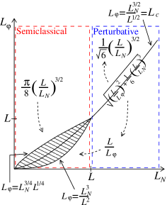
Figure 1: (Color online) On this figure we summarize the different limits for the effective perimeter $\ell_{\rm eff}$ given by eq. (48). For the regime $L\ll L_{N}$, we have used a perturbative method in section III.4. The regime $L\gg L_{N}$ has been studied with the semiclassical approximation (instanton approach) in section III.5. Since the effective perimeter has the structure : $\ell_{\rm eff}=(L/L_{N})^{3/2}\,\eta(L_{c}^{2}/L_{\varphi}^{2})$, the line $L_{\varphi}=L_{c}\propto L_{N}^{3/2}$ separates the regimes of large and small $L_{\varphi}$. The dashed area corresponds to the crossover region where the full expression (56) is needed.

III.5 Large perimeter $L\gg L_{N}$.

In this limit, the function (39), $\tilde{f}(\chi)={\mbox{\large e}}^{-{\rm i}\frac{1}{2}\sqrt{a}(\chi-1/2)^{2}}\,H_{-\frac{1}{2}+{\rm i}\omega}({\mbox{\large e}}^{{\rm i}\pi/4}a^{1/4}(\chi-1/2))$, presents for $\chi\to 0$ a behaviour given by (B.2). For $\chi\to 1$ the function is reduced by an exponential factor ${\mbox{\large e}}^{-\pi\omega}$ (in this limit $\omega\simeq\frac{\sqrt{a}}{8}\gg 1$). It follows from (42) that

$$f^{\prime}(0)\simeq\frac{\tilde{f}^{\prime}(0)}{\tilde{f}(0)}=\frac{L}{L_{N}}\,\frac{{\rm Ai}^{\prime}(L_{N}^{2}/L_{\varphi}^{2})}{{\rm Ai}(L_{N}^{2}/L_{\varphi}^{2})}\>,$$ (55)

(this expression is also derived in appendix C by a different method).

The relation (125) shows that $\tilde{f}^{\prime}(1)\simeq-{\rm i}{\mbox{\large e}}^{-\pi\omega}\tilde{f}^{\prime}(0)$. Therefore we expect that $f^{\prime}(1)/f^{\prime}(0)\sim{\mbox{\large e}}^{-\pi\omega}$ which leads to $\ell_{\rm eff}\simeq\pi\omega$. However this dominant term in $\tilde{f}^{\prime}(1)$ is imaginary and does not contribute to $f^{\prime}(1)$ which is given by the next term in the expansion of $\tilde{f}^{\prime}(1)$. Instead of performing a systematic expansion of $\tilde{f}^{\prime}(1)$, we use the semiclassical solution for the cooperon (see appendix C) which leads to the behaviour (153,156). As a result the effective perimeter is given by the sum of two contributions :

$$\ell_{\rm eff}=\left(\frac{L}{L_{N}}\right)^{3/2}\eta\!\left(\frac{L_{N}^{3}}{L_{\varphi}^{2}L}\right)+\kappa(L_{N}^{2}/L_{\varphi}^{2})\>,$$ (56)

where

$$\eta(x)=\left(\frac{1}{4}+{x}\right)\arctan\frac{1}{\sqrt{4x}}+\frac{\sqrt{x}}{2}$$ (57)

(see appendix C). The second term involves the small and smooth function

$$\kappa(\Lambda)=\ln\left(-4\pi{\mbox{\large e}}^{\frac{4}{3}\Lambda^{3/2}}{\rm Ai}(\Lambda){\rm Ai}^{\prime}(\Lambda)\right)\>.$$ (58)

$\kappa(\Lambda)$ interpolates between $\kappa(\infty)=0$ at large $\Lambda$ and $\kappa(0)=\ln(2/\sqrt{3})\simeq 0.1438$ at $\Lambda=0$ (see figure 2). Since the first term in (56) is much larger than 1 for the regime considered in this subsection, $\kappa(L_{N}^{2}/L_{\varphi}^{2})$ can be neglected in most cases.

Figure 2: The function $\kappa(\Lambda)$ of eq. (58).

Finally the weak localization correction reads

$$\langle\Delta\sigma_{n}\rangle\simeq\frac{e^{2}}{\pi}\,{L_{N}}\,\frac{{\rm Ai}(L_{N}^{2}/L_{\varphi}^{2})}{{\rm Ai}^{\prime}(L_{N}^{2}/L_{\varphi}^{2})}\>{\mbox{\large e}}^{-|n|\ell_{\rm eff}}\>.$$ (59)

We remark that the harmonic $\mathrm{𝟎}$ coincides, as it should in the limit $L\gg L_{N}$, with the result of AAK, eq. (9), for the infinite wire. This provides another check of the exact solution, and in particular of its prefactor.

We now discuss the various limiting cases obtained by varying $L_{\varphi}$. First we remark that the prefactor of eq. (59) has the form $L_{N}\,g_{1}(L_{N}^{2}/L_{\varphi}^{2})$, where $g_{1}(x)$ is a dimensionless function, whereas the effective perimeter has the form ${\ell}_{\rm eff}=(L/L_{N})^{3/2}\,\eta(L_{c}^{2}/L_{\varphi}^{2})$ with $L_{c}=L_{N}\sqrt{L_{N}/L}\ll L_{N}$ (if we neglect the smooth contribution). Therefore we have to distinguish three regimes :

$\bullet$ Negligible exponential dephasing : $L_{\varphi}\gg L_{N}$. Eqs. (56,59) give eq. (33). This is the only regime in which the contribution $\kappa(\Lambda)$ in eq. (56) plays a role.

$\bullet$ $L_{c}=L_{N}\sqrt{L_{N}/L}\ll L_{\varphi}\ll L_{N}$. The prefactor simplifies as

$$\langle\Delta\sigma_{n}\rangle\simeq-\frac{e^{2}}{\pi}\,{L_{\varphi}}\,{\mbox{\large e}}^{-|n|{\ell}_{\rm eff}}$$ (60)

and the effective perimeter can be expanded as

$$\ell_{\rm eff}\simeq\frac{\pi}{8}\left(\frac{L}{L_{N}}\right)^{3/2}+\frac{\pi}{2}\frac{L_{N}^{3/2}L^{1/2}}{L_{\varphi}^{2}}-\frac{4}{3}\left(\frac{L_{N}}{L_{\varphi}}\right)^{3/2}\>.$$ (61)

The two first terms correspond to $\pi\omega$. The effective perimeter is dominated by the first term. However the function $\eta(b/a)$ appears in the argument of an exponential, in eq. (59), multiplied by a large parameter as $\ell_{\rm eff}=\sqrt{a}\,\eta(b/a)$. Therefore it is not clear a priori when the terms of the expansion of $\eta(x)$ are negligible.

$\bullet$ Dominant exponential dephasing : $L_{\varphi}\ll L_{c}$. In this case the expansion of the effective perimeter reads

$$\ell_{\rm eff}\simeq\frac{L}{L_{\varphi}}+\frac{1}{12}\frac{L_{\varphi}L^{2}}{L_{N}^{3}}\>,$$ (62)

which coincides with the expansion of the result $\ell_{\rm eff}\simeq\sqrt{b+a/6}\simeq\sqrt{b}+\frac{a}{12\sqrt{b}}$ obtained by a perturbative expansion in $a$. If $L_{\varphi}\ll L_{N}(L_{N}/L)^{2}$, we recover the result of AAS (6).

We have summarized the different limits for the effective perimeter on figure 1.

IV Relaxation of phase coherence

In this section we interpret the results of the previous section in a time representation and give a rigorous presentation of the heuristic discussion of the introduction. The results of this section may be useful to consider more complicated situations than an isolated ring, when the path integral cannot be computed exactly, like the connected ring studied in the next section. Let us consider the $n$-th harmonic $\widetilde{\cal P}_{n}(x,x^{\prime};t)$ of the cooperon. The Fourier transform over the magnetic flux of the path integrals, eqs. (18,II) in which the coupling to the external magnetic field has been re-introduced, selects the paths with a winding number equal to $n$. We can write :

$$\widetilde{\cal P}_{n}(x,x;t) = \int_{0}^{2\pi}\frac{{\rm d}\theta}{2\pi}\widetilde{\cal P}(x,x;t)\,{\mbox{\large e}}^{-{\rm i}n\theta}$$

$$=\left\langle\int_{x(0)=x}^{x(t)=x}{\cal D}x(\tau)\,{\mbox{\large e}}^{-\frac{1}{4}\int_{0}^{t}{\rm d}\tau\,\dot{x}(\tau)^{2}+{\rm i}\Phi[x(\tau)]}\,\delta_{n,{\cal N}[x(\tau)]}\right\rangle_{V}$$

where ${\cal N}[x(\tau)]$ is the winding number of the trajectory around the ring. For a closed trajectory ($x(0)=x(t)$) we have ${\cal{N}}[x(\tau)]=\frac{1}{L}\int_{0}^{t}{\rm d}\tau\,\dot{x}(\tau)$. (In this section we set $D=1$). Let us introduce the probability ${\cal P}_{n}(x,x^{\prime};t)$ for a Brownian curve to go from $x^{\prime}$ to $x$ in a time $t$ encircling $n$ times the flux :

$${\cal P}_{n}(x,x^{\prime};t)=\int_{x(0)=x^{\prime}}^{x(t)=x}{\cal D}x(\tau)\,{\mbox{\large e}}^{-\frac{1}{4}\int_{0}^{t}{\rm d}\tau\,\dot{x}(\tau)^{2}}\,\delta_{n,{\cal N}[x(\tau)]}\>.$$ (64)

For an isolated ring this probability simply reads

$${\cal P}_{n}(x,x^{\prime};t)=\frac{1}{\sqrt{4\pi t}}\,{\mbox{\large e}}^{-\frac{(x-x^{\prime}-nL)^{2}}{4t}}\>.$$ (65)

Then we can rewrite the harmonics of the conductivity as

$$\widetilde{\cal P}_{n}(x,x;t) = {\cal P}_{n}(x,x;t)\,\left\langle{\mbox{\large e}}^{{\rm i}\Phi[x(\tau)]}\right\rangle_{V,{\cal C}_{n}}$$ (66)

$$= {\cal P}_{n}(x,x;t)\,\left\langle{\mbox{\large e}}^{-\frac{1}{2}\langle\Phi^{2}\rangle_{V}}\right\rangle_{{\cal C}_{n}}$$ (67)

with $\langle\Phi^{2}\rangle_{V}$ given by (20) :

$$\frac{1}{2}\langle\Phi^{2}\rangle_{V}=\frac{2}{\tau_{N}^{3/2}}\int_{0}^{t}{\rm d}\tau\,W(x(\tau),x(\bar{\tau}))\>.$$ (68)

The average

$$\langle\cdots\rangle_{{\cal C}_{n}} = \frac{1}{{\cal P}_{n}(x,x;t)}$$

$$\times\int_{x(0)=x}^{x(t)=x}{\cal D}x(\tau)\,\cdots\,{\mbox{\large e}}^{-\frac{1}{4}\int_{0}^{t}{\rm d}\tau\,\dot{x}(\tau)^{2}}\,\delta_{n,{\cal N}[x(\tau)]}$$

is performed over all closed Brownian trajectories with winding $n$. The probability ${\cal P}_{n}$ in the denominator ensures the normalization $\langle 1\rangle_{{\cal C}_{n}}=1$. Therefore the function $\langle{\mbox{\large e}}^{{\rm i}\Phi}\rangle_{V,{\cal C}_{n}}$, related to the $n$-th harmonic of the AAS oscillations, characterizes the relaxation of phase coherence due to the electron-electron interaction for trajectories with winding number $n$. We now analyze this quantity.

IV.1 Diffusion of the phase

An indication on the nature of the phase relaxation, characterized by the function $\langle{\mbox{\large e}}^{-\frac{1}{2}\langle\Phi^{2}\rangle_{V}}\rangle_{{\cal C}_{n}}$, can be obtained by studying the diffusion of the phase, that is the much simpler quantity $\langle\Phi^{2}\rangle_{V,{\cal C}_{n}}$. If we consider $\tau<t/2$, the average $\langle W\rangle_{{\cal C}_{n}}$ is given by

$${\cal P}_{n}(x,x;t)\left\langle W(x(\tau),x(\bar{\tau}))\right\rangle_{{\cal C}_{n}}=\frac{1}{L}\int_{0}^{L}{\rm d}x{\rm d}x^{\prime}\,W(x,x^{\prime})\,$$

$$\hskip 28.45274pt\times\sum_{m=-\infty}^{+\infty}{\cal P}_{m}(x,x^{\prime};2\tau)\,{\cal P}_{n-m}(x^{\prime},x;t-2\tau)\>.$$ (70)

The final result is symmetric with respect to $2\tau\leftrightarrow t-2\tau$. The double integration can be reduced to a simple integration thanks to the relation $\int_{0}^{1}{\rm d}x{\rm d}x^{\prime}\,f(x-x^{\prime})=\int_{0}^{1}{\rm d}u\,(1-u)[f(u)+f(-u)]$. Then the integral is unfolded to extend over ${\ensmathonze R}$. We obtain :

$${\cal P}_{n}(x,x;t)\left\langle W(x(\tau),x(\bar{\tau}))\right\rangle_{{\cal C}_{n}}=\int_{-\infty}^{+\infty}{\rm d}x\,\Omega(x)\,$$

$$\hskip 14.22636pt\times\frac{1}{2}\left(\frac{{\mbox{\large e}}^{-\frac{x^{2}}{8\tau}}}{\sqrt{8\pi\tau}}\frac{{\mbox{\large e}}^{-\frac{(x-nL)^{2}}{4(t-2\tau)}}}{\sqrt{4\pi(t-2\tau)}}+\left(n\rightarrow-n\right)\right)$$ (71)

where $\Omega(x)$ is the function $\Omega(x)=2W(x,0)(1-\frac{x}{L})=x(1-\frac{x}{L})^{2}$ for $x\in[0,L]$ and periodised on ${\ensmathonze R}$. To go further we distinguish two cases depending on the relative order of magnitude of the time $t$ and the Thouless time $\tau_{D}$.

Diffusive regime ($t\ll\tau_{D}$)

In this case we have to separate the cases $n=0$ and $n\neq 0$.

$\bullet$ Harmonic $n=0$. The integral is dominated by the neighbourhood of $x\sim 0$ since the Gaussian function is very narrow compared to $L$. We can replace the function $\Omega(x)$ by its behaviour near the origin : $\Omega(x)\to\theta(x)x$, where $\theta(x)$ is the Heaviside function. We obtain

$$\left\langle W(x(\tau),x(\bar{\tau}))\right\rangle_{{\cal C}_{0}}\simeq\sqrt{\frac{2\tau(t-2\tau)}{\pi t}}\>.$$ (72)

This result should be symmetrised for $\tau>t/2$. Integration over time $\tau$ gives

$$\frac{1}{2}\langle\Phi^{2}\rangle_{V,{\cal C}_{0}}\simeq\frac{\sqrt{\pi}}{4}\left(\frac{t}{\tau_{N}}\right)^{3/2}\>.$$ (73)

In this regime the geometry plays no role and we recover the result obtained for an infinite wire AkkMon04 ; MonAkk05 . This result is related to the AAK behaviour (9) for $L_{N}\gg L_{\varphi}$.

$\bullet$ Harmonic $n\neq 0$. For times $t\ll\tau_{D}$, the integral (IV.1) can be estimated by the steepest descent method : it is dominated by the neighbourhood of the point minimizing $\frac{x^{2}}{8\tau}+\frac{(x-nL)^{2}}{4(t-2\tau)}$, that is $x=nL\,2\tau/t$. Therefore we obtain :

$$\left\langle W(x(\tau),x(\bar{\tau}))\right\rangle_{{\cal C}_{n}}\simeq\frac{1}{2}\left[\Omega(nL\,2\tau/t)+\Omega(-nL\,2\tau/t)\right]\>.$$ (74)

The integration over time leads to average the function $\Omega$ : $\int_{0}^{t}{\rm d}t\,\left\langle W\right\rangle_{{\cal C}_{n}}=t\int_{0}^{L}\frac{{\rm d}x}{L}\,\Omega(x)$. It immediately follows that :

$$\frac{1}{2}\langle\Phi^{2}\rangle_{V,{\cal C}_{n}}\simeq\frac{1}{6}\frac{\tau_{D}^{1/2}}{\tau_{N}^{3/2}}\,t=\frac{1}{6}\frac{t}{\tau_{c}}\>.$$ (75)

Ergodic regime ($t\gg\tau_{D}$)

The cases $n=0$ and $n\neq 0$ can be treated on the same footing. The Gaussian function in eq. (IV.1) is very broad compared to $L$ and we can replace $\Omega(x)$ by its average value $\Omega(x)\to\frac{1}{L}\int_{0}^{L}{\rm d}x\,\Omega(x)=\frac{L}{12}$. It follows that $\langle W\rangle_{{\cal C}_{n}}\simeq\frac{L}{12}$, then :

$$\frac{1}{2}\langle\Phi^{2}\rangle_{V,{\cal C}_{n}}\simeq\frac{1}{6}\frac{t}{\tau_{c}}\hskip 21.33955pt\forall\ n\>.$$ (76)

To summarize we see that, for the harmonic $n=0$, the diffusion of the phase crosses over from a $t^{3/2}$ behaviour to a linear $t$ behaviour, whereas for $n\neq 0$ it behaves always linearly. This difference shows up in the function $\langle{\mbox{\large e}}^{{\rm i}\Phi}\rangle_{V,{\cal C}_{n}}$ leading either to a non exponential or to an exponential phase coherence relaxation.

IV.2 The function $\langle{\mbox{\large e}}^{{\rm i}\Phi}\rangle_{V,{\cal C}_{n}}$

The calculation of $\langle{\mbox{\large e}}^{{\rm i}\Phi}\rangle_{V,{\cal C}_{n}}$ is a more difficult task. It can be obtained by different strategies.

(A) Small phase approximation.– At short times, the phase $\Phi$ is small, therefore we can linearize the exponential so that : $\langle{\mbox{\large e}}^{-\frac{1}{2}\langle\Phi^{2}\rangle_{V}}\rangle_{{\cal C}_{n}}\simeq{\mbox{\large e}}^{-\frac{1}{2}\langle\Phi^{2}\rangle_{V,{\cal C}_{n}}}$. Then we can use the results given above in subsection IV.1.

(B) Inverse Laplace transform.– The weak localization correction to the conductivity $\langle\Delta\sigma_{n}\rangle\sim\int_{0}^{\infty}{\rm d}t\,{\mbox{\large e}}^{-t/\tau_{\varphi}}\,{\cal P}_{n}(x,x;t)\,\langle{\mbox{\large e}}^{{\rm i}\Phi}\rangle_{V,{\cal C}_{n}}$ has been derived for arbitrary $\tau_{\varphi}=L_{\varphi}^{2}$. Physically, the parameter $\tau_{\varphi}$ takes into account other dephasing mechanisms responsible for an exponential relaxation of phase coherence. From a technical point of view the parameter $\tau_{\varphi}$ allows to probe time scale $t\sim\tau_{\varphi}$ in the path integral and we can, in principle, compute the inverse Laplace tranform of $\langle\Delta\sigma_{n}\rangle$.

(C) Large phase for $n\neq 0$.– If none of the previous methods can be used (the method (B) because it is too difficult, and the method (A) because it is not the range of interest), we can use the following remark : for $\tau_{\varphi}=\infty$ we see from (32) that

$$\langle\Delta\sigma_{n}\rangle\sim\int_{0}^{\infty}{\rm d}t\,\frac{1}{\sqrt{t}}{\mbox{\large e}}^{-\frac{(nL)^{2}}{4t}}\langle{\mbox{\large e}}^{{\rm i}\Phi}\rangle_{V,{\cal C}_{n}}\>.$$ (77)

We expect that the behaviour at large time involves the tail of $\langle{\mbox{\large e}}^{{\rm i}\Phi}\rangle_{V,{\cal C}_{n}}$ which we can assume to behave as $\langle{\mbox{\large e}}^{{\rm i}\Phi}\rangle_{V,{\cal C}_{n}}\propto t^{\mu}{\mbox{\large e}}^{-\Upsilon\,t^{\alpha}}$. The integral of the l.h.s can be estimated by the steepest descent method

$$\int_{0}^{\infty}{\rm d}t\,\frac{1}{\sqrt{t}}{\mbox{\large e}}^{-\frac{(nL)^{2}}{4t}}\>t^{\mu}{\mbox{\large e}}^{-\Upsilon\,t^{\alpha}}$$

$$\simeq\sqrt{\frac{2\pi}{\alpha(\alpha+1)\Upsilon}}\ t_{*}^{\mu-\frac{\alpha}{2}+\frac{1}{2}}\>{\mbox{\large e}}^{-\Upsilon(\alpha+1)t_{*}^{\alpha}}\>,$$ (78)

where $t_{*}=[\frac{1}{\alpha\Upsilon}(\frac{nL}{2})^{2}]^{\frac{1}{\alpha+1}}$. The coefficient $\Upsilon$ and the exponents $\alpha$ and $\mu$ are obtained by comparison of the dependence of this result with $L$ and $n$ with the known behaviour for $\langle\Delta\sigma_{n}\rangle$.

IV.3 Small perimeter $L\ll L_{N}$

We now analyze $\langle{\mbox{\large e}}^{{\rm i}\Phi}\rangle_{V,{\cal C}_{n}}$ in the small perimeter limit.

a. Short times

In the short time limit, the linearization of the exponential is valid (method (A)). Therefore we can use expressions (73,75,76). These expressions give a precise definition of the “short time” regime, which extends until $\langle\Phi^{2}\rangle_{V,{\cal C}_{n}}\sim 1$ that is $t\sim\tau_{c}$. The time scale $\tau_{c}$, given by eq. (16), is associated to the length scale $L_{c}=L_{N}\sqrt{{L_{N}}/{L}}$ introduced in subsection III.5 (see footnote1 ).

b. Long times

In this case we consider the harmonic $n=0$ and $n\neq 0$ on the same footing. The regime $t\gg\tau_{D}$ corresponds to $L\ll L_{\varphi}$. With $L\ll L_{N}$ this leads to the “perturbative” regime $a,b\ll 1$ for which we have found the expressions (51,52) :

$$\int_{0}^{\infty}{\rm d}t\,{\mbox{\large e}}^{-t/\tau_{\varphi}}\,\widetilde{\cal P}_{n}(x,x;t)$$ (79)

$$= \frac{1}{2\sqrt{\frac{1}{L_{\varphi}^{2}}+\frac{1}{6}\frac{L}{L_{N}^{3}}}}\,{\mbox{\large e}}^{-|n|L\sqrt{\frac{1}{L_{\varphi}^{2}}+\frac{1}{6}\frac{L}{L_{N}^{3}}}}\>.$$

The inverse Laplace transform can be computed exactly in this case. It gives

$$\widetilde{\cal P}_{n}(x,x;t)=\frac{1}{2\sqrt{\pi t}}\,{\mbox{\large e}}^{-\frac{(nL)^{2}}{4t}}\,{\mbox{\large e}}^{-\frac{L}{6L_{N}^{3}}t}\>.$$ (80)

We immediately obtain

$$\left\langle{\mbox{\large e}}^{{\rm i}\Phi}\right\rangle_{V,{\cal C}_{n}}=\exp{-\frac{1}{6}\frac{t}{\tau_{c}}}\hskip 14.22636pt\mbox{ for }t\gg\tau_{D}\ \forall n\>.$$ (81)

This is the same result as for $t\ll\tau_{c}$. Since $\tau_{D}\ll\tau_{c}$, it turns out that the result obtained from the linearization of the exponential is valid for all times.

c. Summary

From all these results we can conclude that for harmonic $n=0$ the relaxation is non exponential at very short times and eventually becomes exponential for time larger than the Thouless time :

$$\langle{\mbox{\large e}}^{{\rm i}\Phi}\rangle_{V,{\cal C}_{0}} \simeq \exp{-\frac{\sqrt{\pi}}{4}\left(\frac{t}{\tau_{N}}\right)^{3/2}}\mbox{ for }t\ll\tau_{D}$$ (82)

$$\simeq \exp{-\frac{1}{6}\frac{t}{\tau_{c}}}\hskip 39.83368pt\mbox{ for }t\gg\tau_{D}\>.$$ (83)

This difference comes from the time evolution of $\left\langle W\right\rangle_{{\cal C}_{0}}$ : when the ring has not been explored ($t\ll\tau_{D}$) it scales like $\left\langle W\right\rangle_{{\cal C}_{0}}\sim\sqrt{t}$, while it becomes time independent for ergodic regime ($t\gg\tau_{D}$).

On the other hand the phase coherence relaxation is always exponential for harmonic $n\neq 0$ :

$$\langle{\mbox{\large e}}^{{\rm i}\Phi}\rangle_{V,{\cal C}_{n}}\simeq\exp{-\frac{1}{6}\frac{t}{\tau_{c}}}\hskip 14.22636pt\forall\>t\>.$$ (84)

This is due to the fact that the trajectories with finite winding necessarily explore the ring which leads to $\left\langle W\right\rangle_{{\cal C}_{n}}\sim t^{0}$, for all times, as explained in the introduction.

IV.4 Large perimeter $L\gg L_{N}$

a. Short times

In this regime the analysis provided for small perimeter using the results of section IV.1 remains valid. The condition of validity of the results slightly changes since the times are now in the following order : $\tau_{c}\ll\tau_{N}\ll\tau_{D}$. For harmonic $n=0$, eq. (82) holds for $t\ll\tau_{N}$. For the harmonics $n\neq 0$, eq. (84) holds for $t\ll\tau_{c}$.

b. Long times

$\bullet$ Harmonic $n=0$. For this harmonic, the magnetoconductivity is given by AAK since for $L_{N}\ll L$ the boundary conditions are not important. The inverse Laplace transform of eq. (9) has been computed exactly in ref. AkkMon04 ; MonAkk05 ; footnote4  : $\langle{\mbox{\large e}}^{{\rm i}\Phi}\rangle_{V,{\cal C}_{0}}=\sqrt{\frac{\pi t}{\tau_{N}}}\sum_{n=1}^{\infty}\frac{1}{|u_{n}|}{\mbox{\large e}}^{-|u_{n}|t/\tau_{N}}$, where $u_{n}$’s are zeros of ${\rm Ai}^{\prime}(z)$.

$\bullet$ Harmonic $n\neq 0$. In this case we can only use the method (C). We compare (33) to the integral (IV.2) : the dependence in $n$ of the exponential gives the exponent $\alpha=1$. Then its $L$-dependence gives $\Upsilon=\frac{\pi}{8}\frac{L}{L_{N}^{3}}$. The analysis of the prefactor shows that $\mu=0$. Therefore :

$$\langle{\mbox{\large e}}^{{\rm i}\Phi}\rangle_{V,{\cal C}_{n}}\simeq\exp{-\frac{\pi^{2}}{64}\frac{t}{\tau_{c}}}\>.$$ (85)

c. Summary

For the harmonic $\mathrm{𝟎}$ AkkMon04 ; MonAkk05  :

$$\langle{\mbox{\large e}}^{{\rm i}\Phi}\rangle_{V,{\cal C}_{0}} \simeq \exp{-\frac{\sqrt{\pi}}{4}\left(\frac{t}{\tau_{N}}\right)^{3/2}}\mbox{ for }t\ll\tau_{N}$$ (87)

$$\simeq\sqrt{\frac{\pi t}{\tau_{N}}}\,\frac{1}{|u_{1}|}\,\exp{-|u_{1}|\frac{t}{\tau_{N}}}\hskip 7.11317pt\mbox{ for }\tau_{N}\ll t$$

(the first zero of ${\rm Ai}^{\prime}(z)$ is $|u_{1}|\simeq 1.019$).

For harmonic $n\neq 0$, we have seen above that :

$$\langle{\mbox{\large e}}^{{\rm i}\Phi}\rangle_{V,{\cal C}_{n}} \simeq \exp{-\frac{1}{6}\frac{t}{\tau_{c}}}\hskip 12.80365pt\mbox{ for }t\ll\tau_{c}$$ (88)

$$\simeq \exp{-\frac{\pi^{2}}{64}\frac{t}{\tau_{c}}}\hskip 7.11317pt\mbox{ for }\tau_{c}\ll t\>.$$ (89)

IV.5 From exponential phase coherence relaxation to non exponential size dependent harmonics

On figures 3 and 4 we summarize the results obtained for the function $\langle{\mbox{\large e}}^{{\rm i}\Phi}\rangle_{V,{\cal C}_{n}}$.

The behaviour $\langle\Phi^{2}\rangle_{V}\propto{t}^{3/2}$ was first mentioned in ref. SteAhaImr90 , where it was conjectured that it may lead to interesting effects in a ring. However, when the effect of winding is properly taken into account, it turns out that the interesting effects in the ring come from an exponential relaxation, i.e. $\langle\Phi^{2}\rangle_{V,{\cal{C}}_{n}}\propto{t}$. In order to emphasize this point, let us summarize the relationship between time dependence of the phase relaxation and the decay of the harmonics. For $n\neq 0$, the function $\langle{\mbox{\large e}}^{{\rm i}\Phi}\rangle_{V,{\cal{C}}_{n}}$ is always exponential, $\exp-\beta{t}/{\tau_{c}}$, with $\beta=1/6$ or $\beta={\pi^{2}}/{64}$, depending on the time regime (see figure 4). The weak localization is given by the time integrated probability to turn $n$ times around the ring weighted by the exponential damping :

$$\langle\Delta\sigma_{n}\rangle\sim\int_{0}^{\infty}{\rm d}t\,{\mbox{\large e}}^{-\beta t/\tau_{c}}\,\frac{1}{\sqrt{t}}\,{\mbox{\large e}}^{-\frac{(nL)^{2}}{4t}}\>.$$ (90)

We recover the non exponential size dependence of $\langle\Delta\sigma_{n}\rangle$, eqs. (32,33),

$$\langle\Delta\sigma_{n}\rangle \sim \exp{-\sqrt{\beta}\,|n|\left(\frac{L}{L_{N}}\right)^{3/2}}\sim{\mbox{\large e}}^{-|n|L^{3/2}T^{1/2}}\!\!,$$ (91)

consequence of an exponential relaxation of phase coherence.

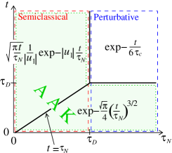
Figure 3: (Color online) Relaxation of phase coherence for trajectories that do not wind around the flux : $\langle{\mbox{\large e}}^{{\rm i}\Phi}\rangle_{V,{\cal C}_{0}}$. The result for the infinite wire (AAK) is recovered when trajectories cannot explore the whole ring, that is either for $t\ll\tau_{D}$ or for $t\ll\tau_{N}$.

Figure 4: (Color online) Relaxation of phase coherence for trajectories with a finite winding number : $\langle{\mbox{\large e}}^{{\rm i}\Phi}\rangle_{V,{\cal C}_{n}}$, with $n\neq 0$.

V The effect of connecting wires

Up to now we have considered an isolated ring. This was an important assumption in order to calculate the path integral. However, in a transport experiment the ring is necessarily connected to wires through which the current is injected. This has two important consequences that we now discuss.

V.1 Classical nonlocality and quantum nonlocality

$\bullet$ Classical nonlocality.– The classical conductance of a wire of section $S$ and length $L$ is given by the Ohm’s law $G^{\rm cl}=\sigma_{0}S/L$ where $\sigma_{0}$ is the Drude conductivity. This result can be rewritten for the dimensionless conductance as $g^{\rm cl}_{\rm wire}=\frac{G^{\rm cl}}{2e^{2}/h}=\alpha_{d}N_{c}\ell_{e}/L$, where $N_{c}$ is the number of channels, $\ell_{e}$ the elastic mean free path and $\alpha_{d}$ a numerical constant depending on the dimension ($\alpha_{1}=2$, $\alpha_{2}=\pi/2$ and $\alpha_{3}=4/3$). The quantum correction to the classical result is given by

$$\langle\Delta g_{\rm wire}\rangle=-\frac{2}{L^{2}}\int_{0}^{L}{\rm d}x\,P_{c}(x,x)\>,$$ (92)

where we have introduced the notation $P_{c}(x,x^{\prime})=\int_{0}^{\infty}{\rm d}t\,{\mbox{\large e}}^{-t/\tau_{\varphi}}\widetilde{\cal P}(x,x^{\prime};t)$.

For a multiterminal network with arbitrary topology, the classical transport is described by a conductance matrix that can be obtained by classical Kirchhoff laws. This classical conductance matrix is a nonlocal object since each matrix element depends on the whole network and the way it is connected to external contacts. On such a network, because of the absence of translation invariance, we have shown in ref. TexMon04 how the cooperon must be properly weighted when integrated over the wires of the network in order to get the weak localization correction to the conductance matrix elements. Eq. (92) generalizes as a sum of contributions of the different wires :

$$\langle\Delta g\rangle=-\frac{2}{{\cal L}^{2}}\sum_{i}\frac{\partial{\cal L}}{\partial l_{i}}\int_{{\rm wire}\ i}{\rm d}x\,P_{c}(x,x)\>,$$ (93)

where ${\cal L}$ is the equivalent length obtained from Kirchhoff laws : $g^{\rm cl}=\alpha_{d}N_{c}\ell_{e}/{\cal L}$. The weight of the wire $i$ is the derivative of the equivalent length with respect to the length of the wire $l_{i}$. The existence of these weights can lead to unexpected results, like a change in sign of the weak localization correction for multiterminal geometries TexMon04 ; TexMon04b ; TexMonAkk05 .

When we consider the ring of figure 5, the equivalent length is given by ${\cal L}=l_{a}+l_{c\parallel d}+l_{b}$ where $l_{c\parallel{d}}^{-1}=l_{c}^{-1}+l_{d}^{-1}$. It follows that

$$\langle\Delta g\rangle=-\frac{2}{(l_{a}+l_{c\parallel d}+l_{b})^{2}}$$

$$\times\left[\int_{a}+\frac{l_{d}^{2}}{(l_{c}+l_{d})^{2}}\int_{c}+\frac{l_{c}^{2}}{(l_{c}+l_{d})^{2}}\int_{d}+\int_{b}\right]{\rm d}x\,P_{c}(x,x)\>.$$

$\bullet$ Quantum nonlocality of the cooperon.– The cooperon is a nonlocal object that depends on the whole network. $P_{c}(x,x)$ is a sum of contributions of diffusive loops that explore the network over distances of order of the phase coherence length. We have shown recently in refs. TexMon04b ; TexMon05 that the presence of the connecting wires can strongly affect the behaviour of the harmonics of the AAS oscillations. We can distinguish two regimes for long connecting wires : (i) in the limit $L_{\varphi}\ll L$ the AAS harmonics are exponential $\langle\Delta{g}_{n}\rangle\propto\exp{-|n|L/L_{\varphi}}$. (ii) However in the limit $L\ll L_{\varphi}$, the behaviour of the harmonics becomes $\langle\Delta{g}_{n}\rangle\propto\exp{-|n|\sqrt{2L/L_{\varphi}}}$. This different behaviour was analyzed in detail and shown to originate from the fact that the Brownian trajectories can explore the connecting wires over distances larger than the perimeter $L$. The effective perimeter of a Brownian trajectory encircling the ring is $\ell_{\rm{eff}}\simeq\sqrt{2L/L_{\varphi}}\gg{L/L_{\varphi}}$.

We see that the simple exponential decay of the harmonics with the perimeter, eq. (6), can be modified for two reasons : either the presence of connecting wires, or the effect of the electron-electron interaction. One acts on the nature of the diffusion around the ring, the other acts on the nature of the dephasing. In this section we propose to combine these two effects.

The presence of connecting wires modifies the diffuson, and therefore the function $W(x,x^{\prime})$. The main difficulty to compute the path integral giving the cooperon is that $W(x,x^{\prime})$ can not be written as a single function of $x-x^{\prime}$ and it is not possible to make the path integral local in time.

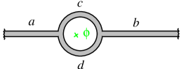
Figure 5: (Color online) A mesoscopic ring connected at two reservoirs (represented by the wavy lines).

V.2 Large perimeter $L\gg L_{N}$

The connecting wires are not expected to have a striking effect in this regime. Since the cooperon vanishes exponentially over distances larger than $L_{N}$ (or $L_{\varphi}$), the integration of the cooperon over the connecting wires can be neglected when studying the harmonics. On the other hand the diffuson is affected by the presence of connecting wires, and the function (27) has to be replaced by (107,109). This function has a similar structure to (27) ; moreover the two functions are equal in the limit of long connecting wires as discussed in appendix A. The function was given in ref. LudMir04 for a symmetric ring ($l_{a}=l_{b}$ and $l_{c}=l_{d}$). In this case, when both $x$ and $x^{\prime}$ are in the same arm of the ring it reads LudMir04 $W(x,x^{\prime})=\frac{1}{2}|x-x^{\prime}|(1-\frac{\gamma+1}{L}|x-x^{\prime}|)$, where $\gamma={l_{c\parallel d}}/{{\cal L}}$. This explains why, in the regime $L\gg{L_{N}}$, the presence of connecting wires has almost no effect. It essentially modifies the numerical prefactor in the exponential : $\langle\Delta g_{n}\rangle\propto\exp-n\frac{C_{\gamma}}{C_{0}}\frac{\pi}{8}(\frac{L}{L_{N}})^{3/2}$. The coefficient ${C_{\gamma}}/{C_{0}}$ interpolates smoothly between $1$ (for $\gamma=0$) and $1/\sqrt{2}$ (for $\gamma=1$) LudMir04 .

Prefactor of the harmonics.– Before going to the limit of small perimeter we consider into more details the prefactor of the conductance. The exact result (59) was derived for an isolated ring and it is not clear how it is related to the conductance through a ring connected to contacts by arms. In this latter case the conductance is given by eq. (V.1). In the limit $L_{N}\ll l_{a},l_{b}\ll l_{c},l_{d}$, let us approximate the cooperon by

$$P_{c}(x,x) \simeq P_{c}|_{\infty\ {\rm wire}}\hskip 24.18501pt\mbox{ for }x\in a,b$$ (95)

$$\simeq P_{c}|_{{\rm isolated\ ring}}\hskip 7.11317pt\mbox{ for }x\in c,d\>,$$ (96)

where $P_{c}|_{\infty\ {\rm wire}}$ and $P_{c}|_{{\rm isolated\ ring}}$ are the cooperon for an infinite wire and the isolated ring, respectively. This means that we neglect the fact that the cooperon can leak in the wires $a$ and $b$, when its coordinate is inside the ring. The harmonic $n=0$, given by

$$\langle\Delta g_{0}\rangle\simeq\frac{L_{N}}{{\cal L}}\,\frac{{\rm Ai}(L_{N}^{2}/L_{\varphi}^{2})}{{\rm Ai}^{\prime}(L_{N}^{2}/L_{\varphi}^{2})}\>,$$ (97)

has the form $\langle\Delta g_{0}\rangle=(\pi/e^{2})\langle\Delta\sigma_{0}\rangle/{\cal L}$. The harmonics $n\neq 0$ read

$$\langle\Delta g_{n}\rangle \simeq \frac{l_{c\parallel d}\,L_{N}}{{\cal L}^{2}}\,\frac{{\rm Ai}(L_{N}^{2}/L_{\varphi}^{2})}{{\rm Ai}^{\prime}(L_{N}^{2}/L_{\varphi}^{2})}\>{\mbox{\large e}}^{-|n|\ell_{\rm eff}}\>,$$ (98)

where the effective perimeter is given by eq. (56).

One may question the validity of the hypothesis (95,96). To answer this question, let us consider the limit $L_{N}/L_{\varphi}=\infty$ of eqs. (97,98) and compare with the exact result obtained in ref. TexMonAkk05 . In eqs. (97,98), the ratio of Airy functions is replaced by $-L_{\varphi}/L_{N}$ and $\ell_{\rm eff}=L/L_{\varphi}$. On the other hand the exact result gives $\langle\Delta g_{0}\rangle\simeq-L_{\varphi}/{\cal L}$ and, for the harmonics $n\neq 0$,

$$\langle\Delta g_{n}\rangle\simeq-\frac{l_{c\parallel d}\,L_{\varphi}}{{\cal L}^{2}}\left(\frac{2}{3}\right)^{2|n|}{\mbox{\large e}}^{-|n|L/L_{\varphi}}\>.$$ (99)

The comparison between eq. (99) and eq. (98) for $L_{N}/L_{\varphi}=\infty$ shows that we only missed the factor $(2/3)^{2|n|}$. This factor is related to the probability for the diffusive trajectory to remain inside the ring, when arriving at the vertex (see refs. AkkComDesMonTex00 ; TexMon05 ; TexMonAkk05 ). Note that, in the limit of short connecting wires $l_{a}\ll L_{\varphi}$, the factor $(2/3)^{2|n|}$ in eq. (99) is replaced by $[1+{L_{\varphi}^{2}}/({l_{a}L})]({2l_{a}}/{L_{\varphi}})^{|n|}$, which describes the probability that the diffusive particule is not absorbed by the nearby reservoir when arriving at the vertex. In the limit $l_{a}/L_{\varphi}\to 0$, the reservoirs break phase coherence at the vertices and the harmonics vanish.

Finally we remark that the prefactor of the harmonics differs from the one obtained by LM LudMir04 . With our notations their result reads : $\langle\Delta g_{n}\rangle_{\rm LM}\sim L_{N}^{9/4}\,{\mbox{\large e}}^{-|n|(\frac{L}{L_{N}})^{3/2}}$, whereas our prefactor is linear in $L_{N}$ (for $L_{\varphi}=\infty$), as for $\langle\Delta\sigma_{n}\rangle$. We stress that the difference between LM’s and our result is not due to the presence of connecting wires. The linear dependence in $L_{N}$ of the prefactors of eqs. (59,98) comes from the path integral. In LM’s paper, the $L_{N}^{9/4}$ comes from a wrong estimation of the prefactor of the path integral. In appendix C we have shown how the correct prefactor can be extracted within the instanton approach followed by LM.

V.3 Small perimeter $L\ll L_{N}$

In this limit, the Brownian trajectories contributing to the path integral (18,II) are related to times $t\gg\tau_{D}$. It is known that for such time scales the arms have a striking effect since the diffusive trajectories spend most of the time in the long connecting wires (see ref. TexMon05 and section 5.5 of ref. ComDesTex05 ). This affects both the winding properties around the ring and the nature of the dephasing.

We expect that the relaxation of the phase coherence mainly occurs inside the arms, i.e. the largest contribution to $\langle\Phi^{2}\rangle_{V}\propto\int_{0}^{t}{\rm d}\tau\,W(x(\tau),x(\bar{\tau}))$ correspond to $x$ and $x^{\prime}$ in the arms. In this case the function $W(x,x^{\prime})$ is given by eqs. (110,111). If we consider the long arm limit $l_{a},l_{b}\gg{L_{N}}\gg{l_{c}},l_{d}$, we can take the limit $l_{a},l_{b}\to\infty$ in (110,111) and we have : $W(x,x^{\prime})\simeq\frac{1}{2}|x-x^{\prime}|$. We recover the same function as for the infinite wire. In this limit the length over which the trajectories extend in the wires is not limited by the size of the system but by the time. Therefore we expect that the phase coherence relaxation is non exponential and the function $\langle{\mbox{\large e}}^{{\rm i}\Phi}\rangle_{V,{\cal{C}}_{n}}$ is similar to the one obtained for the infinite wire (or for the harmonic $n=0$ for the large ring, eqs. (87,87)) : $\langle{\mbox{\large e}}^{{\rm i}\Phi}\rangle_{V,{\cal{C}}_{n}}\simeq\langle{\mbox{\large e}}^{{\rm i}\Phi}\rangle_{V,\mathcal{C}}|_{\rm wire}=f_{\rm wire}(t/\tau_{N})$. This funtion decreases monotoneously over the scale $\tau_{N}$.

Since the cooperon $P_{c}(x,x)$ is expected to decay over a scale $L_{N}$ in the arms, the integration over $x$ in eq. (V.1) leads to (integration is dominated by the contributions of the arms) :

$$\langle\Delta g_{n}\rangle\sim-\frac{L_{N}}{(l_{a}+l_{b})^{2}}\int_{0}^{\infty}{\rm d}t\,\mathcal{P}_{n}(x,x;t)\,\langle{\mbox{\large e}}^{{\rm i}\Phi}\rangle_{V,\mathcal{C}_{n}}$$ (100)

where $x$ is now a point inside the ring (in the regime $t\gg\tau_{D}\propto{L}^{2}$, the probability $\mathcal{P}_{n}(x,x;t)$ is almost independent on $x$, provided it remains at a distance smaller than $\sqrt{t}$ from the ring). The probability to wind $n$ times around the connected ring is TexMon05 $\mathcal{P}_{n}(x,x;t)\simeq\frac{\sqrt{L}}{2^{3/2}t^{3/4}}\,\psi(\xi=\frac{n\sqrt{2L}}{t^{1/4}})$ where $\psi(\xi)\simeq\frac{4}{\sqrt{6\pi}}(\xi/4)^{1/3}{\mbox{\large e}}^{-3(\xi/4)^{4/3}}$ for $\xi\gg 1$ [$\psi(0)$ is finite TexMon05 ]. Therefore, as a function of time, $\mathcal{P}_{n}(x,x;t)$ increases until $t\sim{n}^{4}\tau_{D}$ and then presents a smooth tail $t^{-3/4}$. In order to evaluate eq. (100), we have now to consider two limits :

$\bullet$ For $n^{2}L\ll L_{N}$, the integral (100) is dominated by the tail of the probability $\mathcal{P}_{n}(x,x;t)$, therefore

$$\langle\Delta g_{n}\rangle\sim-\frac{L_{N}^{3/2}L^{1/2}}{(l_{a}+l_{b})^{2}}$$ (101)

$\bullet$ For $n^{2}L\gg L_{N}$, only the tail of $f_{\rm wire}(t/\tau_{N})\sim\sqrt{t/\tau_{N}}\exp-|u_{1}|t/\tau_{N}$ is important. The steepest descent method gives :

$$\langle\Delta g_{n}\rangle\sim-\frac{L_{N}^{3/2}L^{1/2}}{(l_{a}+l_{b})^{2}}\left(\frac{n^{2}L}{L_{N}}\right)^{7/12}\,{\mbox{\large e}}^{-\kappa|n|\sqrt{L/L_{N}}}$$ (102)

whith $\kappa=\sqrt{2}|u_{1}|^{1/4}\simeq 1.421$. We recover a dependence of the harmonics reminiscent to the one obtained for exponential relaxation of phase coherence TexMon05 (see discussion of paragraph V.A). Finally, we remark that the expected decay of the harmonics in temperature is : $\langle\Delta g_{n}\rangle\sim-T^{-11/36}{\mbox{\large e}}^{-nL^{1/2}T^{1/6}}$, for sufficiently large $n$.

This prediction should be tested experimentally on a chain of rings separated by sufficiently long wires, compared to the phase coherence length (several rings are required in order to perform a disorder average).

	Exponential relaxation
$L\gg L_{\varphi}$	$\exp-nL/L_{\varphi}$
$L\ll L_{\varphi}$	$\exp-n(2L/L_{\varphi})^{1/2}$
	Electron-electron interaction
$L\gg L_{N}$	$\exp-\frac{\pi}{8}n(L/L_{N})^{3/2}$
$L\ll L_{N}$	$\exp-\kappa\,n(L/L_{N})^{1/2}$

Table 1: The harmonics $\langle\Delta g_{n}\rangle$ of the conductance through a ring of perimeter $L$ connected to long arms. We compare the results for exponential phase coherence relaxation, described by $L_{\varphi}$, and the one obtained for electron-electron interaction ($L_{N}$). $\kappa$ is the dimensionless constant given in the text.

VI Conclusion

We have considered the effect of the electron-electron interaction on the weak localization correction for a diffusive ring. We have calculated exactly the path integral giving the weak localization correction for the isolated ring in the presence of electron-electron interaction (characterized by the Nyquist length $L_{N}$) and of other dephasing mechanisms described by an exponential phase coherence relaxation (characterized by $L_{\varphi}$). The harmonics of the conductivity are always of the form $\langle\Delta\sigma_{n}\rangle\propto\exp-|n|\ell_{\rm eff}$, where $\ell_{\rm eff}$ accounts for both kinds of relaxation, combined in a nontrivial way. The effective perimeter can always be written as :

$$\ell_{\rm eff}=\left(\frac{L}{L_{N}}\right)^{3/2}f(L_{c}^{2}/L_{\varphi}^{2})\>,$$ (103)

where $L_{c}=L_{N}^{3/2}/L^{1/2}$. For large perimeter $L\gg L_{N}$, the dimensionless function is $f(x)=\eta(x)$ [eq. (157)]. For small perimeter $L\ll L_{N}$ it is given by $f(x)=\sqrt{1/6+x}$. All limiting behaviours of $\ell_{\rm eff}$ have been studied in sections III.4 and III.5.

In order to interpret these results, we have studied the function $\langle{\mbox{\large e}}^{{\rm i}\Phi}\rangle_{V,{\cal C}_{n}}$ characterizing the phase coherence relaxation for trajectories with winding $n$ (involved in the $n$-th harmonic of the AAS oscillations). We have shown that, whereas the phase relaxation crosses over from a non exponential behaviour to an exponential behaviour for the harmonics $n=0$, it is always exponential for $n\neq 0$. The time $\tau_{c}$ characterizing the exponential relaxation $\langle{\mbox{\large e}}^{{\rm i}\Phi}\rangle_{V,{\cal{C}}_{n}}\sim\exp-t/\tau_{c}$ is given by : $\tau_{c}=\sigma_{0}S/(e^{2}TL)=\tau_{N}^{3/2}\tau_{D}^{-1/2}$. This exponential relaxation is at the origin of the non exponential decay of the harmonics with the size and the new temperature dependence footnote5 predicted by LM : $\langle\Delta{g}_{n}\rangle\sim\exp-n(L/L_{N})^{3/2}\sim\exp-nT^{1/2}L^{3/2}$.

In the light of these results it seems difficult to interpret the experiment recently performed on large GaAs/GaAlAs square networks where a behaviour $\exp{-nT^{1/3}}$ was observed FerAngRowGueBouTexMonMai04 ; Fer04 . However the experiment was performed in a temperature range where $L_{N}\sim{L}$. In this regime the diffusive trajectories start to explore the network surrounding the loop, which modifies the behaviour of the harmonics as a function of $L/L_{N}$ and therefore the temperature dependence. However we have not been able to extend the theory to the square network.

In the last part of our article we have studied the effect of the wires connecting the ring to reservoirs. Whereas the AAS harmonics are weakly affected by the connecting wires in the limit $L\gg{L_{N}}$, we have shown that a strong modification is expected in the opposite limit $L\ll{L_{N}}$, where we have predicted a behaviour $\langle\Delta{g}_{n}\rangle\sim{T}^{-11/36}\exp-nL^{1/2}T^{1/6}$. The appropriate experimental setup to test this result is a chain of rings separated by wires whose length remain larger than $L_{N}$. This situation is particularly interesting because the flux sensitivity is due to the motion inside the ring whereas, in this case, the dephasing occurs mostly in the arms.

An interesting effect has been observed recently in the study of four terminal measurements of AB oscillations in a ballistic ring. It has been shown experimentally KobAikKatIye02 that the dephasing rate depends on the configuration of the voltage probes and current probes. It was suggested that a measurement with current probes on both sides of the ring favors charge fluctuations inside the ring and leads to a high dephasing rate, whereas a nonlocal measurement with current probes at one side and voltage probes at the other side (i.e. no current flows through the ring on average) diminishes charge fluctuations in the ring and therefore leads to smaller dephasing rate. This effect has been described theoretically in ref. SeePilJorBut03 . An interesting question is whether a similar effect might occur in a diffusive ring.

Appendix A The function $W(x,x^{\prime})$

A.1 Isolated ring

We give here the solution of the equation $(\gamma-{\rm D}_{x}^{2})P(x,x^{\prime})=\delta(x-x^{\prime})$ on a ring pierced by a flux. ${\rm D}_{x}={\rm d}/{\rm d}x-{\rm i}\theta/L$ is the covariant derivative. We introduce the variable $\chi=x/L\in[0,1]$. The solution of the equation $(b-{\rm D}_{\chi}^{2})C(\chi,\chi^{\prime})=\delta(\chi-\chi^{\prime})$ with $b=\gamma L^{2}$ and ${\rm D}_{\chi}={\rm d}/{\rm d}\chi-{\rm i}\theta$ is given by (45) for $f(\chi)=\frac{\sinh\sqrt{b}(1-\chi)}{\sinh\sqrt{b}}$. The two Green’s functions are related by $P(x,x^{\prime})=L\,C(x/L,x^{\prime}/L)$.

$\bullet$ $\gamma=0$ & $\theta\neq 0$.– Let us consider the limit $\gamma=0$. We have :

$$C(\chi,\chi^{\prime}) = \frac{{\mbox{\large e}}^{{\rm i}\theta(\chi-\chi^{\prime})}}{2(1-\cos\theta)}$$

$$\times\left[1+|\chi-\chi^{\prime}|\left({\mbox{\large e}}^{-{\rm i}\theta\mathop{\mathrm{sign}}\nolimits(\chi-\chi^{\prime})}-1\right)\right]\>.$$

$\bullet$ $\gamma=0$ & $\theta=0$.– In the limit of vanishing $\gamma$ and $\theta$, the diffusion equation possesses a zero mode, therefore the Green’s function $C(\chi,\chi^{\prime})$ presents a diverging contribution : $C(\chi,\chi^{\prime}){{\raisebox{-8.5359pt}{$\textstyle=$}}\atop{\scriptstyle{\theta\to 0}}}\frac{1}{\theta^{2}}-\frac{1}{2}|\chi-\chi^{\prime}|\left(1-|\chi-\chi^{\prime}|\right).$ This diverging contribution disappears when considering the function

$$W(x,x^{\prime}) = \frac{P(x,x)+P(x^{\prime},x^{\prime})}{2}-P(x,x^{\prime})$$ (105)

$$= \frac{1}{2}|x-x^{\prime}|\left(1-\frac{|x-x^{\prime}|}{L}\right)\>.$$ (106)

The existence of a zero mode is an artefact coming from the fact that the system is isolated. In a more realistic situation (when the ring is connected to reservoirs through wires, for example) the Laplace operator does not possess a zero mode AkkComDesMonTex00 . Physically, the zero mode does not contribute to the function $W(x,x^{\prime})$, i.e. to the dephasing, since it corresponds to uniform fluctuations of the electric potential that do not contribute to the phase $\Phi$, given by eq. (19).

A.2 Connected ring

We now construct the symmetric function $W(x,x^{\prime})$, defined in eqs. (21,105), when the ring is connected to reservoirs by two wires (figure 5). In this case $W(x,x^{\prime})$ is fully characterized by a set of components corresponding to the coordinates in the different wires. A system of coordinate must be specified : we first give an orientation to the wires of the network, shown on figure 6 (we call “arc” an oriented wire). Then the coordinate along an arc $i$ belongs to the interval $[0,l_{i}]$, where $l_{i}$ is the length of the arc. Below we construct $W(x,x^{\prime})$ when $x$ and $x^{\prime}$ are both in the ring or both in the arms.

Figure 6: Orientation of the arcs of the ring.

A.2.1 Inside the ring

When both coordinates are in the arc $c$, we obtain :

$$W_{c,c}(x,x^{\prime})=\frac{1}{2}|x-x^{\prime}|\left(1-\frac{l_{a}+l_{d}+l_{b}}{l_{a}+l_{c\parallel d}+l_{b}}\frac{|x-x^{\prime}|}{l_{c}+l_{d}}\right)\>,$$ (107)

with $x,x^{\prime}\in[0,l_{c}]$. For $l_{c}=l_{d}$ we recover the expression given in ref. LudMir04 . We also need the case when $x\in{c}$ and $x^{\prime}\in{d}$ :

$$W_{c,d}(x,x^{\prime}) = \frac{1}{2}\frac{(l_{a}+l_{b})l_{c\parallel d}}{l_{a}+l_{c\parallel d}+l_{b}}\left(1-\frac{x}{l_{c}}-\frac{x^{\prime}}{l_{d}}\right)^{2}$$ (108)

$$+\frac{1}{2}\left[x\left(1-\frac{x}{l_{c}}\right)+x^{\prime}\left(1-\frac{x^{\prime}}{l_{d}}\right)\right]\>,$$

with $x\in[0,l_{c}]$, $x^{\prime}\in[0,l_{d}]$ and with the orientation of figure 6. It is more convenient to consider a unique way to measure both coordinates. Therefore we shift $x^{\prime}$ by $l_{c}$ in (108) :

$$W_{c,d}(x,x^{\prime}-l_{c}) = \frac{1}{2}\bigg{[}-\frac{l_{c}^{2}}{l_{a}+l_{c\parallel d}+l_{b}}-\frac{l_{a}-l_{c\parallel d}+l_{b}}{l_{a}+l_{c\parallel d}+l_{b}}x+\left(1+\frac{2\,l_{c}^{2}}{(l_{c}+l_{d})(l_{a}+l_{c\parallel d}+l_{b})}\right)x^{\prime}$$ (109)

$$-\frac{l_{a}+l_{d}+l_{b}}{l_{a}+l_{c\parallel d}+l_{b}}\frac{x^{2}}{l_{c}+l_{d}}-\frac{l_{a}+l_{c}+l_{b}}{l_{a}+l_{c\parallel d}+l_{b}}\frac{x^{\prime 2}}{l_{c}+l_{d}}+\frac{l_{a}+l_{b}}{l_{a}+l_{c\parallel d}+l_{b}}\frac{2xx^{\prime}}{l_{c}+l_{d}}\bigg{]}\>,$$

with $x\in[0,l_{c}]$ and $x^{\prime}\in[l_{c},l_{c}+l_{d}]$. It is now clear that in the limit of long connecting wires, $l_{a},l_{b}\gg l_{c},l_{d}$, eqs. (107,109) lead to the same result as in the isolated ring, eq. (106). We see that, inside the ring, $W(x,x^{\prime})$ is not everywhere a function of $x-x^{\prime}$ only, apart in the limit $l_{a},l_{b}\to\infty$.

A.2.2 Inside the arms

When both coordinates are in the same arm, we have :

$$W_{a,a}(x,x^{\prime})=\frac{1}{2}|x-x^{\prime}|\left(1-\frac{|x-x^{\prime}|}{l_{a}+l_{c\parallel d}+l_{b}}\right)$$ (110)

When the two coordinates belong to different arcs we prefer to shift the origin of the coordinate $x^{\prime}$, as we did inside the ring. If the shift is chosen to be $l_{a}+l_{c\parallel d}$, we obtain the simple expression :

$$W_{a,b}(x,x^{\prime}-l_{a}-l_{c\parallel d})=\frac{1}{2}(x^{\prime}-x)\left(1-\frac{x^{\prime}-x}{l_{a}+l_{c\parallel d}+l_{b}}\right)$$ (111)

(in this expression $x^{\prime}=l_{a}+l_{c\parallel d}$ corresponds to the begining of the arc $b$). When $l_{c\parallel{d}}=0$ (no ring) we obtain from (110,111) the result for a connected wire $W(x,x^{\prime})=\frac{1}{2}|x-x^{\prime}|(1-\frac{|x-x^{\prime}|}{l_{a}+l_{b}})$, which is similar to the one for the isolated ring eq. (106), as mentioned above. It is remarkable that, in the presence of the ring, there exists a choice of coordinates for which $W(x,x^{\prime})$ in the arms has precisely the same structure as in the absence of the ring. In the limit of an infinite wire, $l_{a},l_{b}\to\infty$, we recover from (110,111) the result of the infinite wire, $W(x,x^{\prime})\simeq\frac{1}{2}|x-x^{\prime}|$.

Appendix B Hermite function

Consider the Hermite equation NikOuv83  :

$$y^{\prime\prime}(z)-2z\,y^{\prime}(z)+2\nu\,y(z)=0\>.$$ (112)

Two linearly independent solutions are the Hermite function $H_{\nu}(z)$ and $H_{\nu}(-z)$. An integral representation is

$$H_{\nu}(z)=\frac{1}{\Gamma(-\nu)}\int_{0}^{\infty}\frac{{\rm d}t}{t^{\nu+1}}\,{\mbox{\large e}}^{-t^{2}-2zt}\>,$$ (113)

from which we get the series representation :

$$H_{\nu}(z)=\frac{1}{2\Gamma(-\nu)}\sum_{n=0}^{\infty}(-1)^{n}\Gamma\left(\frac{n-\nu}{2}\right)\frac{(2z)^{n}}{n!}\>.$$ (114)

We now study several limiting behaviours of the Hermite function $H_{-\frac{1}{2}+{\rm i}\omega}({\mbox{\large e}}^{{\rm i}\pi/4}a^{1/4}(\chi-1/2))$, where $\omega=\frac{1}{2}(\frac{b}{\sqrt{a}}+\frac{\sqrt{a}}{4})$.

B.1 The limit $a\to 0$

In this case $\omega\simeq\frac{b}{2\sqrt{a}}$, therefore we study the limit $\omega\to\infty$ when the argument of the Hermite function reads $z=x/\sqrt{-{\rm i}\omega}$ with $x$ finite. Using the expression $\Gamma\left(\frac{n}{2}+\frac{1}{4}-{\rm i}\frac{\omega}{2}\right)\propto\left(\frac{\omega}{2}\right)^{\frac{n}{2}}{\mbox{\large e}}^{-{\rm i}n\frac{\pi}{4}}$, valid for $\omega\gg n$, and the series representation (114), we get

$$H_{-\frac{1}{2}+{\rm i}\omega}\left(\frac{x}{\sqrt{-{\rm i}\omega}}\right){{\raisebox{-8.5359pt}{$\textstyle\propto$}}\atop{\scriptstyle{\omega\to\infty}}}{\mbox{\large e}}^{-\sqrt{2}\,x}\>.$$ (115)

B.2 The limit $a\to\infty$ : from Hermite to Airy function

The first step to study this limit is to perform a rotation of $+\pi/4$ in the complex plane of the axis of integration in (113). One obtains

$$H_{-\frac{1}{2}+{\rm i}\omega}\left({\mbox{\large e}}^{{\rm i}\pi/4}A\right)=\frac{{\mbox{\large e}}^{{\rm i}\frac{\pi}{8}+\frac{\pi}{4}\omega}}{\Gamma\left(\frac{1}{2}-{\rm i}\omega\right)}\int_{0}^{\infty}\frac{{\rm d}x}{\sqrt{x}}\,{\mbox{\large e}}^{-{\rm i}\varphi(x,\chi)}$$ (116)

where the phase reads

$$\varphi(x,\chi)=x^{2}+2A\,x+\omega\ln x\>.$$ (117)

We introduced the notation

$$A=a^{1/4}\left(\chi-\frac{1}{2}\right)\>.$$ (118)

We are interested in the limit $a\to\infty$ with $L_{N}/L_{\varphi}$ finite (or zero), therefore it is convenient to write :

$$\omega=\frac{\sqrt{a}}{8}\left(1+4\frac{\Lambda}{a^{1/3}}\right)$$ (119)

where $\Lambda=({L_{N}}/{L_{\varphi}})^{2}$.

(i) The case $\chi\to 0$

The function $\varphi(x,\chi)$ is a monotonous function of the variable $x\in{\ensmathonze R}^{+}$, however its second derivative vanishes at $x=\pm\sqrt{\omega/2}$. For $\chi\to 0$ the first derivative at this point becomes very small in the limit $a\to\infty$, therefore we expect that the neighbourhood of $\sqrt{\omega/2}$ brings the dominant contribution to the integral. The expansion of the phase in the neighbourhood of $\sqrt{\omega/2}$ reads (for $t\to 0$)

$$\varphi\left(\sqrt{\omega/2}+a^{1/12}t,\chi\right) = \varphi\left(\sqrt{\omega/2},\chi\right)$$

$$+\left(a^{1/3}\chi+\Lambda\right)t+\frac{1}{3}t^{3}-\frac{1}{2a^{1/6}}t^{4}+\cdots+O(a^{\frac{3-n}{6}}t^{n})\>.$$

Inserting this expression into the integral representation (116), we obtain the Airy function AbrSte64 ${\rm Ai}(x)=\frac{1}{2\pi}\int_{-\infty}^{+\infty}{\rm d}t\,{\mbox{\large e}}^{{\rm i}(\frac{t^{3}}{3}+xt)}$, namely :

$$H_{-\frac{1}{2}+{\rm i}\omega}\left({\mbox{\large e}}^{{\rm i}\pi/4}a^{1/4}(\chi-\frac{1}{2})\right)$$

$$\hskip 28.45274pt{{\raisebox{-8.5359pt}{$\textstyle\propto$}}\atop{\scriptstyle{a\to\infty}}}{\mbox{\large e}}^{-{\rm i}\frac{\sqrt{a}}{2}\chi}\>{\rm Ai}\left(\Lambda+a^{1/3}\chi\right)\>.$$ (121)

This expression is valid for $\chi\to 0$ such that $a^{1/3}\chi$ is not large, and for $\Lambda/a^{1/3}\ll 1$. This last condition rewrites $L_{\varphi}\gg L_{N}\sqrt{L_{N}/L}$.

(ii) The case $\chi\to 1$

For $\chi\to 1$ the expansion of $\varphi(z,\chi)$ must be realized in the neighbourhood of $-\sqrt{\omega/2}$, where the first derivative with respect to $z$ vanishes (the first derivative at $+\sqrt{\omega/2}$ now diverges in the limit $a\to\infty$). Therefore the contour of integration must be deformed in order to visit the neighbourhood of $z=-\sqrt{\omega/2}$. The new contour of integration is shown on the right part of figure 7. For $\chi>1/2$ :

$$\int_{0}^{\infty}\frac{{\rm d}x}{\sqrt{x}}\,{\mbox{\large e}}^{-{\rm i}\varphi(x,\chi)}=\int_{{\cal C}^{\prime}_{1}+{\cal C}^{\prime}_{2}}\frac{{\rm d}z}{\sqrt{z}}\,{\mbox{\large e}}^{-{\rm i}\varphi(z,\chi)}\>.$$ (122)

To deal with more symmetric expressions for $\chi>1/2$ and $\chi<1/2$ we remark that the contour of integration can also be deformed in this latter case (see the left part of figure 7). For $\chi<1/2$ :

$$\int_{0}^{\infty}\frac{{\rm d}x}{\sqrt{x}}\,{\mbox{\large e}}^{-{\rm i}\varphi(x,\chi)}=\int_{{\cal C}_{1}+{\cal C}_{2}}\frac{{\rm d}z}{\sqrt{z}}\,{\mbox{\large e}}^{-{\rm i}\varphi(z,\chi)}\>.$$ (123)

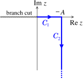
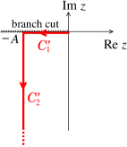
Figure 7: (Color online) Left : Contour of integration in the complex plane for $\chi<1/2$ (i.e. $A<0$). The vertical line separates the regions where $\mathop{\mathrm{Re}}\nolimits[{\rm i}(z^{2}+2Az)]$ is positive or negative in the lower half of the complex plane. Right : Contour of integration for $\chi>1/2$ (i.e. $A>0$)

The dominant contribution to the integral is given by the contribution of the segment ${\cal C}^{\prime}_{1}$. By noting that $\varphi(z{\mbox{\large e}}^{-{\rm i}\pi},\chi)=-{\rm i}\pi\omega+\varphi(z,1-\chi)$ for $\chi>1/2$ and $z\in{\ensmathonze R}^{+}$, we see that, for $\chi>1/2$,

$$\int_{{\cal C}^{\prime}_{1}}\frac{{\rm d}z}{\sqrt{z}}\,{\mbox{\large e}}^{-{\rm i}\varphi(z,\chi)}=-{\rm i}{\mbox{\large e}}^{-\pi\omega}\int_{{\cal C}_{1}}\frac{{\rm d}z}{\sqrt{z}}\,{\mbox{\large e}}^{-{\rm i}\varphi(z,1-\chi)}\>.$$ (124)

Therefore, since $\tilde{f}(\chi)$ is dominated by ${\cal C}_{1}$ for $\chi\to 0$ and by ${\cal C}_{1}^{\prime}$ for $\chi\to 1$ we have

$$\tilde{f}(\chi)\simeq-{\rm i}{\mbox{\large e}}^{-\pi\omega}\tilde{f}(1-\chi)\hskip 14.22636pt\mbox{for }\chi\to 1\>.$$ (125)

Appendix C Semiclassical approach

In this appendix we analyze the cooperon solution of (III.2) by following a semiclassical approach, valid for $L_{N}\ll L$. We construct the solution of the equation $[-\frac{{\rm d}^{2}}{{\rm d}\chi^{2}}+V(\chi)]f(\chi)=0$ for $\chi\in[0,1]$, where the potential is

$$V(\chi)=a\chi(1-\chi)+b\>.$$ (126)

The solution of interest satisfies $f(0)=1$ and $f(1)=0$. As shown in the text, the harmonics of the cooperon then read

$$C^{(n)}(0,0)=\frac{1}{2\sqrt{f^{\prime}(0)^{2}-f^{\prime}(1)^{2}}}\,{\mbox{\large e}}^{-|n|\ell_{\rm eff}}$$ (127)

with $\cosh\ell_{\rm eff}=\frac{f^{\prime}(0)}{f^{\prime}(1)}$.

The semiclassical approach holds for $a\gg 1$. In this case the quadratic potential acts as a high barrier in which the solution hardly penetrates.

Semiclassical solution : instanton.– The WKB solution of the differential equation can be expressed as $f(\chi)\simeq\frac{1}{\sqrt{\pi(\chi)}}\exp\pm\int^{\chi}{\rm d}\chi^{\prime}\,\pi(\chi^{\prime})$ where the conjugate momentum for zero “energy” is $\pi(\chi)=\sqrt{V(\chi)}$. Let us introduce :

$${\cal S}(\chi)=\int_{0}^{\chi}{\rm d}\chi^{\prime}\,\sqrt{V(\chi^{\prime})}\>,$$ (128)

which is the action of the instanton penetrating inside the potential barrier (classical solution for imaginary time) for zero “energy”. We write the semiclassical solution in the form

$$f(\chi)=\frac{a^{1/6}}{\sqrt{\pi}\,[V(\chi)]^{1/4}}\,\left(B_{\rm sc}\,{\mbox{\large e}}^{-{\cal S}(\chi)}+C_{\rm sc}\,{\mbox{\large e}}^{+{\cal S}(\chi)}\right)\>,$$ (129)

where $B_{\rm sc}$ and $C_{\rm sc}$ are two coefficients to be determined in order to satisfy boundary conditions.

Validity of the semiclassical approximation.– The validity of the semiclassical approximation can be expressed precisely by the condition $|\frac{{\rm d}}{{\rm d}\chi}\frac{1}{\pi(\chi)}|\ll 1$. This condition rewrites here as

$$a^{1/3}\left(\chi(1-\chi)+\frac{b}{a}\right)\gg 1\>.$$ (130)

Depending on the relative magnitude of $L_{N}$ and $L_{\varphi}$, there are two possibilities that we discuss now. We recall the notation $\Lambda=b/a^{2/3}=L_{N}^{2}/L_{\varphi}^{2}$

C.1 Regime $L_{\varphi}\ll L_{N}$

In this case $b/a^{2/3}\gg 1$ and the condition (130) is fulfilled for any $\chi\in[0,1]$. We immediately find the coefficients $B_{\rm sc}$ and $C_{\rm sc}$ by imposing the boundary conditions and obtain :

$$f(\chi)=\sqrt{\frac{\pi(0)}{\pi(\chi)}}\>\frac{\sinh[{\cal S}(1)-{\cal S}(\chi)]}{\sinh{\cal S}(1)}\>.$$ (131)

Therefore

$$f^{\prime}(0) = -\frac{a}{4b}-\sqrt{b}\,\coth{\cal S}_{\rm inst}\simeq-\sqrt{b}$$ (132)

$$f^{\prime}(1) = -\frac{\sqrt{b}}{\sinh{\cal S}_{\rm inst}}\simeq-2\sqrt{b}\,{\mbox{\large e}}^{-{\cal S}_{\rm inst}}\>,$$ (133)

where we have introduced the notation ${\cal S}_{\rm inst}\equiv{\cal S}(1)$. The effective perimeter simply reads :

$$\ell_{\rm eff}=\mathop{\mathrm{argcosh}}\nolimits\frac{f^{\prime}(0)}{f^{\prime}(1)}\simeq{\cal S}_{\rm inst}\>.$$ (134)

C.2 Arbitrary $L_{\varphi}$

In the case $L_{\varphi}\gtrsim L_{N}$ (i.e. $b/a^{2/3}\lesssim 1$) the condition (130) cannot be fulfilled near the edges of the interval. For $\chi\sim 0$ the condition (130) can only be satisfied for $\chi\gtrsim\chi_{c}$ whereas for $\chi\sim 1$ it is satisfied for $1-\chi\gtrsim\chi_{c}$. We have defined $\chi_{c}$ by the two conditions $a^{1/3}\chi_{c}+\Lambda\gg 1$ and $\chi_{c}\ll 1$ (the breakdown of the semiclassical approximation near the edges can be simply understood by noting that, for $b=0$, $\chi=0$ and $\chi=1$ are the turning points of the classical solution for imaginary time for a zero “energy”). Therefore the resolution of the differential equation must be performed carefully near the edges. We separate the interval $[0,1]$ into three parts :

(i) In the neighbourhood of $\mathrm{𝟎}$ where the potential is linear, the solution is a combination of two Airy functions AbrSte64  :

$$f(\chi)=B_{1}\,{\rm Ai}(a^{1/3}\chi+\Lambda)+C_{1}\,{\rm Bi}(a^{1/3}\chi+\Lambda)\>.$$ (135)

(ii) Semiclassical solution.– Sufficiently far from the edges of the interval, that is in the interval $[\chi_{c},1-\chi_{c}]$, we can use the WKB solution (129).

(iii) In the neighbourhood of $\chi=1$ the potential is almost linear again and the solution reads

$$f(\chi) = B_{2}\,{\rm Ai}(a^{1/3}(1-\chi)+\Lambda)$$ (136)

$$+C_{2}\,{\rm Bi}(a^{1/3}(1-\chi)+\Lambda)\>.$$

The solution $f(\chi)$ is continuous and differentiable. Therefore the matching of the three expressions should now be performed in the region $\chi\sim\chi_{c}$ and $\chi\sim 1-\chi_{c}$. It is clear from the definition of $\chi_{c}$ that the matching is realized in the Airy functions’ asymptotic region. We obtain the following relations between the coefficients :

$$\left(\begin{array}[]{c}B_{2}\\ C_{2}\end{array}\right)=\left(\begin{array}[]{cc}0&q\\ 1/q&0\end{array}\right)\left(\begin{array}[]{c}B_{1}\\ C_{1}\end{array}\right)\>,$$ (143)

where

$$q=2\,{\mbox{\large e}}^{{\cal S}_{\rm inst}+\frac{4}{3}\Lambda^{3/2}}\,\gg 1\>.$$ (144)

We add to these relations the conditions

$$f(0) = B_{1}\,{\rm Ai}(\Lambda)+C_{1}\,{\rm Bi}(\Lambda)=1$$ (145)

$$f(1) = B_{2}\,{\rm Ai}(\Lambda)+C_{2}\,{\rm Bi}(\Lambda)=0\>.$$ (146)

Solving these equations we find :

$$B_{1} = \frac{q^{2}\,{\rm Ai}}{q^{2}\,{\rm Ai}^{2}-{\rm Bi}^{2}}$$ (147)

$$C_{1} = \frac{-{\rm Bi}}{q^{2}\,{\rm Ai}^{2}-{\rm Bi}^{2}}$$ (148)

where Airy functions are taken at $\Lambda$. We eventually find :

$$f^{\prime}(0) = a^{1/3}\,\frac{q^{2}\,{\rm Ai}\,{\rm Ai}^{\prime}-{\rm Bi}\,{\rm Bi}^{\prime}}{q^{2}\,{\rm Ai}^{2}-{\rm Bi}^{2}}\simeq a^{1/3}\,\frac{{\rm Ai}^{\prime}}{{\rm Ai}}$$ (149)

$$f^{\prime}(1) = -a^{1/3}\,\frac{q/\pi}{q^{2}\,{\rm Ai}^{2}-{\rm Bi}^{2}}\simeq-a^{1/3}\frac{1}{\pi\,q\,{\rm Ai}^{2}}\>,$$ (150)

where we have used that the Wronskian of the Airy functions is ${\cal W}[{\rm Ai},{\rm Bi}]={\rm Ai}\,{\rm Bi}^{\prime}-{\rm Ai}^{\prime}\,{\rm Bi}=1/\pi$ (see ref. AbrSte64 ). Finally the two derivatives are

$$f^{\prime}(0) \simeq a^{1/3}\,\frac{{\rm Ai}^{\prime}(\Lambda)}{{\rm Ai}(\Lambda)}$$ (151)

$$f^{\prime}(1) \simeq -\frac{a^{1/3}}{2\pi}\,\frac{{\mbox{\large e}}^{-{\cal S}_{\rm inst}-\frac{4}{3}\Lambda^{3/2}}}{{\rm Ai}(\Lambda)^{2}}\>.$$ (152)

We can check that (151,152) coincide with (132,133) in the limit $L_{\varphi}\ll L_{N}$. The effective perimeter is given by

$$\ell_{\rm eff}={\cal S}_{\rm inst}+\ln\left(-4\pi{\rm Ai}(\Lambda){\rm Ai}^{\prime}(\Lambda){\mbox{\large e}}^{\frac{4}{3}\Lambda^{3/2}}\right)\>.$$ (153)

Eq. (151) corresponds to the limit (55) derived directly from the exact solution, which gives the prefactor of the harmonics (59).

Action of the instanton.– We analyze more into detail the action corresponding to the crossing of the barrier :

$${\cal S}(1) = \int_{0}^{1}{\rm d}\chi\,\sqrt{V(\chi)}$$ (155)

$$=\pi\omega\left(1-\frac{2}{\pi}\arcsin\frac{1}{\sqrt{1+{a}/({4b})}}\right)+\frac{\sqrt{b}}{2}$$

where we recall that $\omega=\frac{\sqrt{a}}{8}+\frac{b}{2\sqrt{a}}$. The action can be written in the form

$${\cal S}_{\rm inst}\equiv{\cal S}(1)=\sqrt{a}\ \eta({b}/{a})$$ (156)

where the function $\eta(x)$ is given by :

$$\eta(x)=\left(\frac{1}{4}+{x}\right)\arctan\frac{1}{\sqrt{4x}}+\frac{\sqrt{x}}{2}\>.$$ (157)

This function presents the following limiting behaviours :

$$\eta(x)=\pi\left(\frac{1}{8}+\frac{x}{2}\right)-\frac{4}{3}\,x^{3/2}+O(x^{5/2})\mbox{ for }x\ll 1$$ (158)

$$\eta(x)=\sqrt{x}+\frac{1}{12}\frac{1}{\sqrt{x}}+O(x^{-3/2})\hskip 28.45274pt\mbox{ for }x\gg 1\>.$$ (159)

Appendix D A perturbative approach to solve equation (37)

We solve equation (37) with the boundary conditions (41) in the limit $a\ll 1$. Let us write the solution as an expansion in powers of the parameter $a$ :

$$f(\chi)=f_{0}(\chi)+f_{1}(\chi)+f_{2}(\chi)+\cdots\>,$$ (160)

where $f_{n}(\chi)=O(a^{n})$. In order to satisfy the boundary conditions (41) at any level of approximation we impose $f_{0}(0)=1$ and $f_{0}(1)=0$ for the order 0, and $f_{n}(0)=f_{n}(1)=0$ for higher orders. $f_{0}(\chi)$ is solution of $f_{0}^{\prime\prime}-bf_{0}=0$, therefore :

$$f_{0}(\chi)=\frac{\sinh\sqrt{b}(1-\chi)}{\sinh\sqrt{b}}\>.$$ (161)

The first order term satisfies the differential equation :

$$f_{1}^{\prime\prime}(\chi)-bf_{1}(\chi)=a\chi(1-\chi)f_{0}(\chi)\equiv\Psi(\chi)\>.$$ (162)

The solution satisfying the appropriate boundary conditions reads :

$$f_{1}(\chi) = -\frac{1}{{\cal W}}\Bigg{[}f_{0}(\chi)\int_{0}^{\chi}{\rm d}t\>\Psi(t)\,f_{0}(1-t)$$ (163)

$$+ f_{0}(1-\chi)\int_{\chi}^{1}{\rm d}t\>\Psi(t)\,f_{0}(t)\Bigg{]}\>,$$

where ${\cal W}=\frac{\sqrt{b}}{\sinh\sqrt{b}}$ is the Wronskian of the two solutions ${\cal W}={\cal W}[f_{0}(\chi),f_{0}(1-\chi)]$. After some calculations the derivatives are found :

$$f^{\prime}(0) = -\sqrt{b}\coth\sqrt{b}-\frac{a}{4\sinh^{2}\sqrt{b}}$$

$$\times\left(-\frac{1}{3}+\frac{\cosh^{2}\sqrt{b}}{b}-\frac{\sinh 2\sqrt{b}}{2b^{3/2}}\right)+O(a^{2})$$

$$f^{\prime}(1) = -\sqrt{b}\frac{1}{\sinh\sqrt{b}}+\frac{a}{4\sinh^{2}\sqrt{b}}$$

$$\times\left(\frac{1}{3}\cosh\sqrt{b}-\frac{\cosh\sqrt{b}}{b}+\frac{\sinh\sqrt{b}}{b^{3/2}}\right)+O(a^{2})\>.$$

Appendix E Relation between the weak localization and the conductivity fluctuations

We re-examine the relation between the weak localization and the conductivity fluctuations studied in ref. AleBla02 for the case of the wire and used in ref. LudMir04 . We show that the relation is more general and holds for the local conductivity $\sigma=\int\frac{{\rm d}r{\rm d}r^{\prime}}{{\rm Vol}}\sigma(r,r^{\prime})$. Note that it is only meaningful to consider a local conductivity when the distribution of currents is uniform (translation invariant system or a network with equal currents in its wires).

The weak localization is governed only by the phase coherence length ($L_{N}$ and/or $L_{\varphi}$). The study of conductivity fluctuations involves another important length scale : the thermal length $L_{T}=\sqrt{D/T}$. Conductivity fluctuations are given by four contributions : the two first are interpreted as correlations of the diffusion constant AltShk86

$$\langle\delta\sigma(B)\,\delta\sigma(B^{\prime})\rangle^{(1)} = \frac{16}{{\rm Vol}^{2}}\left(\frac{e^{2}}{h}\right)^{2}\frac{\pi D^{2}}{3T}\int_{0}^{\infty}{\rm d}t{\rm d}t^{\prime}\,\tilde{\delta}(t-t^{\prime})$$ (166)

$$\times\int{\rm d}r{\rm d}r^{\prime}\,\widetilde{\cal P}_{d}(r,r^{\prime};t)\,\widetilde{\cal P}_{d}(r,r^{\prime};t^{\prime})^{*}$$

where $\tilde{\delta}(t)=\frac{3T}{\pi}\left(\frac{\pi Tt}{\sinh\pi Tt}\right)^{2}$ is a function of width $1/T$ and normalized to unity. The second contribution is obtained by replacing the diffuson by the cooperon $\widetilde{\cal P}_{c}$. The two remaining contributions, of the form $\int_{0}^{\infty}{\rm d}t{\rm d}t^{\prime}\,\tilde{\delta}(t-t^{\prime})\int{\rm d}r{\rm d}r^{\prime}\,\mathop{\mathrm{Re}}\nolimits[\widetilde{\cal P}_{d}(r,r^{\prime};t)\,\widetilde{\cal P}_{d}(r^{\prime},r;t^{\prime})]$, are interpreted as correlations of the density of states AltShk86 . However, these two contributions are negligible AleBla02 since $L_{T}\ll L_{N}$ is necessary fulfilled ($L_{T}\sim L_{N}$ corresponds to the threshold of strong localization). The condition $L_{T}\ll L_{N}$ allows us to replace the function $\tilde{\delta}(t)$ by $\delta(t)$ and obtain :

$$\langle\delta\sigma(B)\,\delta\sigma(B^{\prime})\rangle^{(1)} = \frac{16}{{\rm Vol}^{2}}\left(\frac{e^{2}}{h}\right)^{2}\frac{\pi D^{2}}{3T}$$ (167)

$$\times\int_{0}^{\infty}{\rm d}t\,\int{\rm d}r{\rm d}r^{\prime}\,\left|\widetilde{\cal P}_{d}(r,r^{\prime};t)\right|^{2}\>.$$

The diffuson and cooperon are solutions of the “diffusion” equation

$$\left[\frac{\partial}{\partial t}-D\left(\nabla-2{\rm i}eA_{\mp}\right)^{2}+{\rm i}\left(V_{1}(r,t)-V_{2}(r,t)\right)\right]\widetilde{\cal P}_{d,c}(r,r^{\prime};t)=\delta(t)\,\delta(r-r^{\prime})\>.$$ (168)

$A_{\mp}$ is the vector potential related to the magnetic field $(B\mp B^{\prime})/2$, where the sign is $-$ for $\widetilde{\cal P}_{d}$ and $+$ for $\widetilde{\cal P}_{c}$. The two potentials $V_{1}$ and $V_{2}$ are the two fluctuating electric potential associated to the two conductivity bubbles. They are both characterized by the same fluctuations, given by the fluctuation-dissipation theorem (17), however $V_{1}$ and $V_{2}$ are uncorrelated since they are associated to the conductivity bubbles for two different configurations of the disorder footnote6  : $\left\langle V_{i}(r,t)\,V_{j}(r^{\prime},t^{\prime})\right\rangle_{V}=\delta_{ij}\frac{2e^{2}}{\sigma_{0}}T\,\delta(t-t^{\prime})\,P_{d}(r,r^{\prime})$.

Starting from the path integral representation of the diffuson it is possible to perform the average over the fluctuating potential :

$$\left\langle\left|\widetilde{\cal P}_{d}(r,r^{\prime};t)\right|^{2}\right\rangle_{V}=\int_{r_{1}(0)=r^{\prime}}^{r_{1}(t)=r}{\cal D}r_{1}(\tau)\,\int_{r_{2}(0)=r^{\prime}}^{r_{2}(t)=r}{\cal D}r_{2}(\tau)\,{\mbox{\large e}}^{-\frac{1}{4D}\int_{0}^{t}{\rm d}\tau\,\dot{r}_{1}^{2}-\frac{1}{4D}\int_{0}^{t}{\rm d}\tau\,\dot{r}_{2}^{2}-\frac{4e^{2}T}{\sigma_{0}}\int_{0}^{t}{\rm d}\tau\,W(r_{1}(\tau),r_{2}(\tau))}\>,$$ (169)

where $W(r,r^{\prime})$ was defined above by eq. (21). We introduce $r(\tau)$ defined for $\tau\in[0,2t]$ such that $r(\tau)=r_{1}(\tau)$ if $\tau\in[0,t]$ and $r(\tau)=r_{2}(2t-\tau)$ if $\tau\in[t,2t]$. The the two path integrals can be gathered in one thanks to the integration over $r$ : $\int{\rm d}r\int_{r^{\prime},0}^{r,t}{\cal D}r_{1}(\tau)\int_{r^{\prime},0}^{r,t}{\cal D}r_{2}(\tau)\rightarrow\int_{r^{\prime},0}^{r^{\prime},2t}{\cal D}r(\tau)$.

$$\int{\rm d}r\left\langle\left|\widetilde{\cal P}_{d}(r,r^{\prime};t)\right|^{2}\right\rangle_{V}=\int_{r(0)=r^{\prime}}^{r(2t)=r^{\prime}}{\cal D}r(\tau)\,{\mbox{\large e}}^{-\frac{1}{4D}\int_{0}^{2t}{\rm d}\tau\,\dot{r}^{2}-\frac{2e^{2}T}{\sigma_{0}}\int_{0}^{2t}{\rm d}\tau\,W(r(\tau),r(2t-\tau))}\>.$$ (170)

This leads to the following relation :

$$\langle\delta\sigma(B)\,\delta\sigma(B^{\prime})\rangle^{(1)}=-2\frac{e^{2}}{h}\frac{\pi}{3}\frac{L_{T}^{2}}{{\rm Vol}}\langle\Delta\sigma\left(\frac{B-B^{\prime}}{2}\right)\rangle$$ (171)

where the weak localization is given by (II,23). Similarly the contribution of the cooperon gives :

$$\langle\delta\sigma(B)\,\delta\sigma(B^{\prime})\rangle^{(2)}=-2\frac{e^{2}}{h}\frac{\pi}{3}\frac{L_{T}^{2}}{{\rm Vol}}\langle\Delta\sigma\left(\frac{B+B^{\prime}}{2}\right)\rangle\>.$$ (172)

The total correlation function $\langle\delta\sigma(B)\,\delta\sigma(B^{\prime})\rangle$ is the sum of these two contributions. The relations (171,172) were proved by Aleiner & Blanter in ref. AleBla02 by an explicit calculation of the path integral for a wire and a plane, and comparison to the result of AAK AltAroKhm82 . Here we have demonstrated these relations without having explicitly calculated the path integral, which makes our proof more general, valid as soon as it is meaningful to consider a local conductivity. The important physical consequence of these relations is that the weak localization (i.e. the Altshuler–Aronov–Spivak oscillations) and the conductance fluctuations (i.e. the Aharonov–Bohm oscillations) are governed by the same length scale $L_{N}$. For example we expect the amplitude of the AB oscillations to behave like

$$\delta g^{\rm AB}_{n}\propto L_{T}\sqrt{L_{N}}\,\exp-|n|\frac{\pi}{16}\left(\frac{L}{L_{N}}\right)^{3/2}$$ (173)

for $L\gg L_{N}$.

References

- (1) S. Hikami, A. I. Larkin, and Y. Nagaoka, Spin-Orbit Interaction and Magnetoresistance in the Two Dimensional Random System, Prog. Theor. Phys. 63(2), 707 (1980).
- (2) B. L. Al’tshuler and A. G. Aronov, Magnetoresistance of thin films and of wires in a longitudinal magnetic field, JETP Lett. 33(10), 499 (1981).
- (3) B. L. Al’tshuler, A. G. Aronov, and B. Z. Spivak, The Aaronov-Bohm Effect in disordered conductors, JETP Lett. 33(2), 94 (1981).
- (4) B. L. Altshuler, A. G. Aronov, and D. E. Khmelnitsky, Effects of electron-electron collisions with small energy transfers on quantum localisation, J. Phys. C: Solid St. Phys. 15, 7367 (1982).
- (5) B. L. Altshuler and A. G. Aronov, Electron-electron interaction in disordered conductors, in Electron-electron interactions in disordered systems, edited by A. L. Efros and M. Pollak, page 1, North-Holland, 1985.
- (6) For the calculation of , a factor 2 was missing in ref. AltAroKhm82 and the correct factor can be found in refs. AleAltGer99 ; GouPiePotEstBir00 ; AkkMon04 for example.
- (7) I. L. Aleiner, B. L. Altshuler, and M. E. Gershenson, Interaction effects and phase relaxation in disordered systems, Waves Random Media 9, 201 (1999).
- (8) A. B. Gougam, F. Pierre, H. Pothier, D. Esteve, and N. O. Birge, Comparison of energy and phase relaxation in metallic wires, J. Low Temp. Phys. 118, 447 (2000).
- (9) P. M. Echternach, M. E. Gershenson, H. M. Bozler, A. L. Bogdanov, and B. Nilsson, Nyquist phase relaxation in one-dimensional metal films, Phys. Rev. B 48(15), 11516 (1993).
- (10) É. Akkermans and G. Montambaux, Physique mésoscopique des électrons et des photons, EDP Sciences, CNRS éditions, 2004.
- (11) C. Texier and G. Montambaux, Weak localization in multiterminal networks of diffusive wires, Phys. Rev. Lett. 92, 186801 (2004).
- (12) C. Texier, G. Montambaux, and E. Akkermans, in preparation (2005).
- (13) G. Montambaux and E. Akkermans, Non exponential quasiparticle decay and phase relaxation in low dimensional conductors, Phys. Rev. Lett. 95, 016403 (2005).
- (14) Note that the existence of a non exponential behaviour has been first noticed in ref. SteAhaImr90 on qualitative ground.
- (15) A. Stern, Y. Aharonov, and Y. Imry, Phase uncertainty and loss of interference: A general picture, Phys. Rev. A 41(7), 3436 (1990).
- (16) F. Pierre, A. B. Gougam, A. Anthore, H. Pothier, D. Esteve, and N. O. Birge, Dephasing of electrons in mesoscopic metal wires, Phys. Rev. B 68, 085413 (2003).
- (17) T. Ludwig and A. D. Mirlin, Interaction-induced dephasing of Aharonov-Bohm oscillations, Phys. Rev. B 69, 193306 (2004).
- (18) Note that LM have written their result in a different way : where depends on the perimeter of the ring and is related to by . Therefore . Throughout our article we rather use the notation .
- (19) I. L. Aleiner and Ya. M. Blanter, Inelastic scattering time for conductance fluctuations, Phys. Rev. B 65, 115317 (2002).
- (20) M. Ferrier, Transport électronique dans les fils quasi-unidimensionnels : cohérence de phase dans les réseaux de fils quantiques et supraconductivité des cordes de nanotubes de carbone, PhD thesis, Université Paris-Sud, 2004.
- (21) C. Texier and G. Montambaux, Quantum oscillations in mesoscopic rings and anomalous diffusion, J. Phys. A: Math. Gen. 38, 3455–3471 (2005).
- (22) A. Comtet, J. Desbois, and C. Texier, Functionals of the Brownian motion, localization and metric graphs, J. Phys. A: Math. Gen. 38, R341-R383 (2005).
- (23) A. Nikiforov and V. Ouvarov, Fonctions spéciales de la physique mathématique, Mir, Moscou, 1983.
- (24) J. Desbois, Spectral determinant of Schrödinger operators on graphs, J. Phys. A: Math. Gen. 33, L63 (2000).
- (25) It is interesting to note that AAK’s result has been simultaneously derived by probabilists studying the statistical properties of the absolute area below a Brownian bridge (a Brownian motion conditioned to come back to its initial point) in ref. She82 (moreover this author pointed out that the result was obtained even earlier in the context of economy in ref. CifReg75 ). In this context eq. (9) is interpreted as the double Laplace transform of the distribution below a Brownian bridge. The inverse Laplace transforms were performed in ref. Ric82 .
- (26) L. A. Shepp, On the integral of the absolute value of the pinned Wiener process, Ann. Probab. 10(1), 234 (1982), [Acknowledgement of priority: Ann. Probab. 19, 1397 (1991)].
- (27) D. M. Cifarelli and E. Regazzini, Contributi intorno ad un test per l’homogeneita tra du campioni, Giornale Degli Economiste 34, 233–249 (1975).
- (28) S. O. Rice, The integral of the absolute value of the pinned Wiener process – Calculation of its probability density by numerical integration, Ann. Probab. 10(1), 240 (1982).
- (29) C. Texier and G. Montambaux, How to increase a transmission with weak localization ? A geometrical effect, in Quantum information and decoherence in nanosystems, edited by C. Glattli, M. Sanquer, and J. Trân Thanh Vân, Gioi publishers, Vietnam, 2005, p. 279, proceedings of the XXXIXth Moriond conference, La Thuile, Italy, january 2004.
- (30) We stress that the temperature dependence of the harmonics is characteristic of the diffusive regime (for large perimeter). In the ballistic regime the harmonics of the AB oscillations behaves like , as observed experimentally in ref. HanKriPedSorLin01 and discussed theoretically in ref. SeeBut01 .
- (31) A. E. Hansen, A. Kristensen, S. Pedersen, C. B. Sørensen, and P. E. Lindelof, Mesoscopic decoherence in Aharonov-Bohm rings, Phys. Rev. B 64, 045327 (2001).
- (32) G. Seelig and M. Büttiker, Charge-fluctuation-induced dephasing in a gated mesoscopic interferometer, Phys. Rev. B 64, 245313 (2001).
- (33) M. Ferrier, L. Angers, A. C. H. Rowe, S. Guéron, H. Bouchiat, C. Texier, G. Montambaux, and D. Mailly, Direct measurement of the phase coherence length in a GaAs/GaAlAs square network, Phys. Rev. Lett. 93, 246804 (2004).
- (34) K. Kobayashi, H. Aikawa, S. Katsumoto, and Y. Iye, Probe-Configuration-Dependent Decoherence in an Aharonov-Bohm Ring, J. Phys. Soc. Jpn. 71(9), L2094 (2002).
- (35) G. Seelig, S. Pilgram, A. N. Jordan, and M. Büttiker, Probe-configuration dependent dephasing in a mesoscopic interferometer, Phys. Rev. B 68, 161310 (2003).
- (36) E. Akkermans, A. Comtet, J. Desbois, G. Montambaux and C. Texier, On the spectral determinant of quantum graphs, Ann. Phys. (N.Y.) 284, 10–51 (2000).
- (37) M. Abramowitz and I. A. Stegun, editors, Handbook of Mathematical functions, Dover, New York, 1964.
- (38) B. L. Al’tshuler and B. I. Shklovskiĭ, Repulsion of energy levels and conductivity of small metal samples, Sov. Phys. JETP 64(1), 127 (1986).
- (39) In a perturbative treatment of the electron-electron interaction LeeRam85 , this means that the e-e interaction lines do not couple the two conductivity bubbles.
- (40) P. A. Lee and T. V. Ramakrishnan, Disordered electronic systems, Rev. Mod. Phys. 57, 287 (1985).