Cell dynamics approach to the formation of metastable phases during phase transformation

Abstract

In this paper, we use the cell dynamics method to study the dynamics of phase transformation when three phases exist. The system we study is a two-dimensional system. The system is able to achieve three phases coexistence, which for simplicity we call crystal, liquid and vapor phases. We focus our study on the case when the vapor and crystal phases are stable and can coexist while the other intermediate liquid phase is metastable. In this study we examine the most fundamental process of the growth of a composite nucleus which consists of a circular core of one phase surrounded by a circular layer of second phase embedded in a third phase. We found that there is one special configuration that consists of a core stable phase surrounded by another stable phase in a metastable liquid environment which becomes stationary and stable. Then, the nucleus does not grow and the metastable liquid survives. The macroscopic liquid phase does not disappear even though it is thermodynamically metastable. This result seems compatible to the argument of kinetics of phase transition developed by Cahn [J. Am. Ceram. Soc. 52, 118 (1969)] based on the construction of a common tangent of the free energy curve.

I Introduction

The study of the formation of the long-lived metastable phase during phase transformation has a long history Ostwald (1897); Cahn (1969). Recently, renewed interest in the metastable phase formation, in particular, in the field of soft-condensed matter physics Poon (2002); Evans and Cates (1997) has emerged because of the rather long relaxation time of these materials, which, typically, are in the ranges 1 ms to 1 year Renth et al. (2001). Although the formation of the thermodynamically metastable phase is not only academically but industrially important because many industrial products are in long-lived metastable state, the theoretical study of the kinetics of phase transformation is hindered because of the lack of appropriate theoretical and computational models. Hence, a detailed understanding of the kinetics of phase transformation using realistic modeling is essential.

The direct microscopic computer simulation of the nucleation and the kinetics of phase transformation using molecular dynamics or the Monte Carlo method is possible Auer and Frenkel (2001) but is still a difficult task. Even the most fundamental phenomenon like nucleation is still not easy. In order to avoid the demand for huge computational resources, and to get the qualitative (course-grained) picture of the kinetics of phase transformation, the mesoscopic approach based on the phenomenological model called the Cahn-Hilliard Cahn and Hilliard (1959), Ginzburg-Landau Valls and Mazenko (1990) or phase-field model Castro (2003); Gránásy et al. (2004), which requires a solution using a non-linear partial differential equation, has been traditionally employed. Since this approach requires the time integration of highly non-linear partial differential equations, it is still not easy to simulate the long-time behavior of the kinetics of phase transformation Roger et al. (1988) except for the various forms of special analytical traveling wave solutions Chan (1977); Bechhoefer et al. (1991); Celestini and ten Bosh (1994); Iwamatsu and Horii (1996).

In order to understand the full kinetics of phase transformation with the transient and long-lived metastable phase, an efficient simulation method is absolutely necessary. In this report, we use a formalism which is based on the cell dynamics method to investigate the kinetics of the metastable phase during the phase transformation when the circular grain (nucleus) of the stable phase grows. Our result suggests that the metastable phase can be long-lived indeed, and it also indicates that the cell dynamics method is efficient and flexible enough to study the kinetics of the metastable phase during the phase transformation.

II Cell dynamics method for three-phase system

In order to study the phase transformation, it is customary to study the partial differential equation called the time-dependent Ginzburg-Landau (TDGL) equation:

$$\frac{\partial\psi}{\partial t}=-\frac{\delta\mathcal{F}}{\delta\psi}$$ (1)

where $\psi$ is the non-conserved order parameter and $\mathcal{F}$ is the free energy functional (grand potential), which is usually written as the square-gradient form:

$$\mathcal{F}[\psi]=\int d{\bf r}\left[\frac{1}{2}D(\nabla\psi)^{2}+h(\psi)\right]$$ (2)

The local part of the free energy $h(\psi)$ determines the bulk phase diagram and the value of the order parameters in equilibrium phases. Traditionally, the double-well form

$$h(\psi)=-\frac{1}{2}\psi^{2}+\frac{1}{4}\psi^{4}$$ (3)

has been used to model the phase transformation of a two phase system.

Puri and Oono Puri and Oono (1988) transformed this TDGL equation (1) for the non-conserved order parameter into the space-time discretized cell-dynamics equation following a similar transformation of the kinetic equation for the conserved order parameter called the Cahn-Hilliard-Cook equation Oono and Puri (1988). Their transformation does not correspond to the numerical approximation of the original TDGL equation. Rather, they aimed at simulating the kinetics of phase transformation of real system within the framework of discrete cellular automata.

According to their cell dynamics method, the partial differential equation (1) is transformed into the finite difference equation in space and time:

$$\psi(t+1,n)=F[\psi(t,n)]$$ (4)

where the time $t$ is discrete integer and the space is also discrete and is expressed by the site index (integer) $n$. The mapping $F$ is given by

$$F[\psi(t,n)]=-f(\psi(t,n))+\left[<<\psi(t,n)>>-\psi(t,n)\right]$$ (5)

where $f(\psi)=dh(\psi)/d\psi$ and the definition of $<<*>>$ for the two-dimensional square grid is given by

$$<<\psi(t,n)>>=\frac{1}{6}\sum_{i=\mbox{nn}}\psi(t,i)+\frac{1}{12}\sum_{i=\mbox{nnn}}\psi(t,i)$$ (6)

with ”nn” means the nearest neighbors and ”nnn” the next-nearest neighbors of the square grid. Improved forms of this mapping function $F$ for three-dimensional case was also obtained Puri and Oono (1988); Oono and Puri (1988); Teixeira and Mulder (1997).

Oono and Puri Puri and Oono (1988); Oono and Puri (1988) have further approximated the derivative of the local free energy $f(\psi)$ called ”map function” by the $\tanh$ form:

$$f(\psi)=\frac{dh}{d\psi}\simeq\psi-A\tanh\psi$$ (7)

with $A=1.3$, which corresponds to the free energy Chakrabarti and Brown (1992):

$$h(\psi)=-A\ln\left(\cosh\psi\right)+\frac{1}{2}\psi^{2}$$ (8)

and is the approximation to (3) if $A=1.5$ Chakrabarti and Brown (1992); Teixeira and Mulder (1997). Later Chakrabarti and Brown Chakrabarti and Brown (1992) argued that this simplification is justifiable since the detailed form (3) of the free energy $h(\psi)$ is irrelevant to the long-time kinetics and the scaling exponent.

Subsequently, however, several authors used the map function $f(\psi)$ directly obtained from the free energy $h(\psi)$ in cell dynamics equation (5) as it is Qi and Wang (1996); Ren and Hamley (2001) and found that the cell dynamics equation is still amenable for a realistic map function numerically. Ren and Hamley Ren and Hamley (2001) argued that by using the original form of the free energy function $f(\psi)$ one can easily include the effect of asymmetry of free energy and, hence, the asymmetric character of two phases can be considered. It is now well recognized that this cell dynamics method can reproduce the essential feature of the kinetics of phase transformation between two phases even though the method is not guaranteed Teixeira and Mulder (1997) to be an accurate approximation of the original TDGL partial differential equation (1).

A further extension of the cell dynamics equation to the three phase system is simple. One has to introduce the free energy function $h(\psi)$ of triple-well form, which can achieve a three-phase coexistence. In our report, we will use one of the simplest analytical forms proposed by Widom Widom (1978):

$$h(\psi)=\frac{1}{4}(\psi+1)^{2}(\psi-1)^{2}(\psi^{2}+\epsilon)$$ (9)

where the parameter $\epsilon$ controls the relative stability of three phases. Several shapes of the free energy function $h(\psi)$ for several values of the parameter $\epsilon$ are shown in Fig. 1. As can be seen from the figure, two phases around $\psi_{v}=-1$ which we call vapor and $\psi_{c}=1$ which we call crystal for simplicity always coexist, while another phase around $\psi_{l}=0$ which we call liquid can be metastable when $0\leq\epsilon\leq 0.5$. The free energy of this metastable liquid phase is higher than that of the stable crystal or vapor phases by the amount

$$\Delta h=f(\psi=1)-f(\psi=0)=\frac{\epsilon}{4}$$ (10)

This liquid phase becomes completely unstable and disappears when $\epsilon>\epsilon_{c}$ where $\epsilon_{c}=0.5$ is the critical point. When $\epsilon<0$, only the liquid phase is stable and both the vapor and the crystal phases are metastable instead. Since we are interested in the case when only one intermediate phase is metastable, we will consider the case when $0\leq\epsilon\leq\epsilon_{c}$. As will be shown in the next section, even though the metastable liquid minimum is irrelevant for the equilibrium phase behavior, it not only controls the phase transition kinetics but appears as the long-lived macroscopic metastable phase during the phase transformation.

Similar triple-well potentials were used by several workers to study the nucleation Gránásy and Oxtoby (2000) and the metastable phase formation Evans and Cates (1997); Celestini and ten Bosh (1994); Evans et al. (1997) within the framework of the original TDGL or the phase-field model. The importance of this triple-well free energy and the appearance of the metastable state were also recently suggested experimentally in a colloid-polymer mixture Poon (2002); Renth et al. (2001)

Figure 1: The model triple-well free energy Widom (1978) which can achieve a three-phase coexistence. The left phase with $\psi_{v}=-1$ is called vapor, the central phase with $\psi_{l}=0$ is called liquid and the right phase with $\psi_{c}=1$ is called crystal for convenience. The triple point is at $\epsilon_{t}=0$, when all three phases are at equilibrium and can coexist. The liquid phase becomes metastable when $\epsilon_{t}<\epsilon<\epsilon_{m}$ where $\epsilon_{m}=0.2044$ though the local vapor-liquid or liquid-crystal equilibrium could be realized because the common tangent between the stable vapor and the metastable liquid phases or those between stable crystal and metastable liquid phases can be drawn (broken lines). When the parameter $\epsilon$ exceeds $\epsilon_{m}=0.2044$, no common tangent can be drawn, so the two-phase equilibrium between vapor-liquid and liquid-crystal cannot be achieved. When $\epsilon$ is larger than $\epsilon_{c}=0.5$, the liquid phase becomes completely unstable.

III Numerical results and discussions

III.1 Front velocity of the growing stable phase

Before looking at the issue of the kinetics of phase transformation of a metastable phase in a three-phase system, we will briefly look at the growth of one circular nucleus from the stable phase after nucleation in a two-phase system. In order to simulate the evolution of a nucleus, we have to prepare the system as a two-phase system in which one phase is stable and another is metastable and has higher free energy than the former. The free energy difference between the stable and metastable phases is controlled by the super saturation in usual liquid condensation from vapor and by the under-cooling in usual crystal nucleation. Microscopically, this free energy difference is necessary for the nucleus of the stable phase to grow by overcoming the curvature effect of the surface tension Iwamatsu (1993).

In order to study the growth of a stable phase using a cell dynamics system, we will consider the time-dependent Ginzburg-Landau (TDGL) equation (1) of square gradient form (2). The local part of the free energy $h(\psi)$, which we use is Jou and Lusk (1997); Iwamatsu and Nakamura :

$$h(\psi)=\frac{1}{4}q\psi^{2}(1-\psi)^{2}+\frac{3}{2}\epsilon\left(\frac{\psi^{3}}{3}-\frac{\psi^{2}}{2}\right)+\frac{1}{4}\epsilon$$ (11)

This free energy is shown in Fig. 2 where the liquid phase with $\psi_{l}=0$ is metastable while the crystal phase with $\psi_{c}=1$ is stable, which mimics the liquid-crystal part of the triple-well potential (9). The free energy barrier between two phases can be tuned by $q$, while the free energy difference $\Delta h$ between the stable phase at $\psi_{c}=1$ and the metastable phase at $\psi_{l}=0$ can be controlled by $\epsilon$. This free energy difference is given by the same formula (10) as in the model three-phase system. We choose the parameter $q=2$ in order to mimic the functional form of the triple well free energy in Fig. 1 as shown in Fig. 2.

Figure 2: The model double-well free energy Jou and Lusk (1997); Iwamatsu and Nakamura (solid curve) which achieves the two-phase equilibrium is compared with the triple-well free energy in Fig. 1 (broken curve). The parameter $\epsilon$ determines the free energy difference $\Delta h$, and the parameter $q$ determines the free energy barrier. We choose $q=2$ to mimic the triple-well potential.

The time-dependent Ginzburg-Landau (TDGL) equations (1) and (2) for a circular or a spherical growing nucleus of stable phase in a metastable environment with radial coordinate $r$ is written as Chan (1977)

$$D\left(\frac{\partial^{2}}{\partial r^{2}}+\frac{d-1}{r}\frac{\partial}{\partial r}\right)\psi-\frac{\partial\psi}{\partial t}=\frac{\partial h}{\partial\psi}$$ (12)

where $d$ is the dimension ($d=2$ for a circular and $d=3$ for a spherical nucleus) of the problem. Then, the traveling wave solution having radial symmetry with moving interface at $R(t)$ of the form

$$\psi({\bf r},t)=\psi(X),$$ (13)

with $X=r-R(t)$ satisfies the differential equation

$$D\frac{d^{2}\psi}{dX^{2}}+v\frac{d\psi}{dX}-\frac{\partial h}{\partial\psi}=0$$ (14)

with

$$v=\frac{dR}{dt}+\frac{D(d-1)}{R}.$$ (15)

Equation (14) represents a mechanical analogue of the equation of motion of classical particle in a potential well $-h$ subject to a friction force which is proportional to the parameter $v$. Therefore, a finite size of the free energy difference $\Delta h$ is necessary for (14) to compensate for the dissipation of energy due to friction and to have a solution which corresponds to a traveling wave. In other words, the moving (growing or shrinking) interface is possible only when there is the free energy difference $\Delta h$ between two phases. Therefore, one phase should be metastable and another should be stable.

Equation (14) has a particular solution only when the parameter $v$ takes a specific value. The corresponding interfacial velocity $dR/dt$ is given by

$$\frac{dR}{dt}=v-\frac{D(d-1)}{R}$$ (16)

where, the second term on the right hand side represents the effect of capillary pressure. For a larger nucleus with $R\rightarrow\infty$, the interfacial velocity becomes $v$ which is also the formula for the one-dimension problem with $d=1$. For a smaller nucleus, the actual interfacial velocity $dR/dt$ will be smaller than $v$ due to the capillary pressure because $R>0$. In particular, when $dR/dt<0$, the nucleus cannot grow. The nucleus with a radius $R$ larger than the critical radius $R_{c}$ grows while the one with a smaller radius disappears. The critical radius $R_{c}$ is determined from $dR/dt=0$ which gives

$$R_{c}=\frac{D(d-1)}{v}$$ (17)

Therefore, in two-phase coexistence with $v=0$, any circular or spherical nucleus with finite radius $R$ disappears, and only a flat interface remains.

The shrinking metastable void within a stable phase is also described by the equations (12) to (17), but now, with $v<0$ and $dR/dt<0$. Then, the capillary pressure in (16) always accelerates the interfacial velocity, and there is no critical radius $R_{c}$ for the void.

The above steady-state solution of TDGL with a constant interfacial velocity $v$ was obtained analytically in a one-dimension by Chan Chan (1977) when the free energy is written using the quartic form (11). Using his formula, the interfacial velocity $v$ of our TDGL model (1) and (2) with the free energy (11) is given by:

$$v=\sqrt{\frac{D}{2q}}3\epsilon$$ (18)

Chan Chan (1977) further suggested that if the interfacial width is narrow, the interfacial velocity of a circular or spherical growing nucleus is asymptotically given by the same formula (18). The larger the free energy difference $\epsilon$, and the lower the free energy barrier $q$, the higher the front velocity $v$ from (18).

The critical radius $R_{c}$ of a circular nucleus in a two-dimensional system is also given analytically Chan (1977); Jou and Lusk (1997) by

$$R_{c}=\frac{D}{v}=\frac{\sqrt{2qD}}{3\epsilon}$$ (19)

In the metastable environment, a nucleus of a stable phase with a radius $R$ smaller than $R_{c}$ shrinks, while the nucleus with a radius larger than $R_{c}$ grows and its front velocity approaches (18). The void of a metastable phase surrounded by a stable environment always shrinks regardless of the size of the critical radius. Again, the larger the free energy difference $\epsilon$, and the lower the free energy barrier $q$, the smaller the critical radius $R_{c}$ .

We have imported the above free energy (11) into the cell dynamics code written by Mathematica TM Wolfram (2003) for the animation of spinodal decomposition developed by Gaylord and Nishidate Gaylord and Nishidate (1996), and simulated the growth of the stable crystal phase in a metastable liquid environment and that of a metastable liquid void in a stable crystal environment.

Figures 3 and 4 show the evolution of the stable circular crystal phase in a metastable liquid environment, and the contraction of a metastable liquid void in a stable crystal environment. The system size is 100$\times$100=10000 and $D=0.5$ Puri and Oono (1988); Gaylord and Nishidate (1996). The periodic boundary condition is used. The initial nucleus or void is prepared by randomly selecting the order parameter $\psi$ from $0.9\leq\psi\leq 1.1$ for stable crystal and from $-0.1\leq\psi\leq 0.1$ for metastable liquid. The initial random distribution is necessary because our cell-dynamics system is deterministic and does not include random noise. The figures 3 and 4 show that the stable circular crystal grows and the metastable circular liquid shrinks steadily without changing the circular shape appreciably.

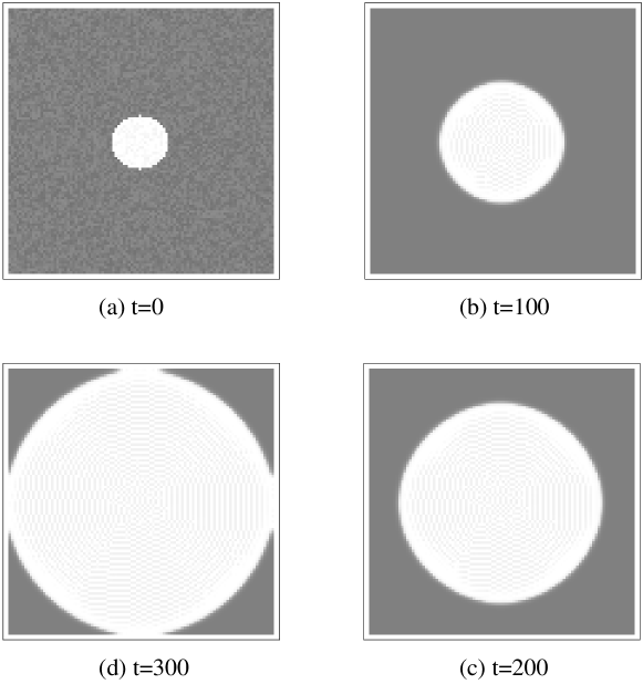
Figure 3: The evolution of the crystal nucleus (white) in the metastable liquid environment (gray) when $q=2$ and $\epsilon=0.1$.

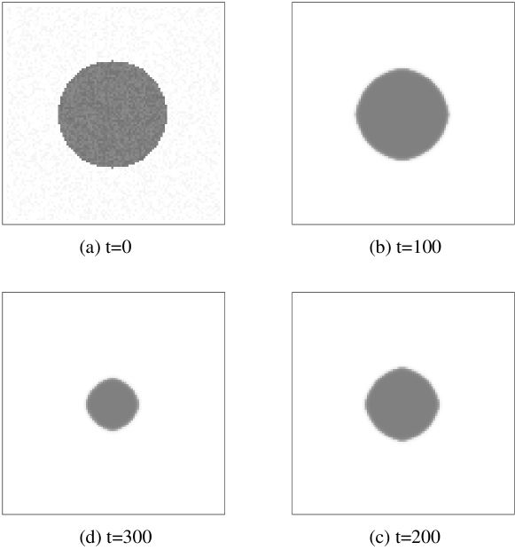
Figure 4: The contraction of the metastable liquid void (gray) in the stable crystal environment (white) when $q=2$ and $\epsilon=0.1$.

In Fig. 5 the effective radius $r$ of the circular nucleus of a stable crystal grain and a metastable liquid void, which is calculated by assuming the circular area $S$ from

$$r=\sqrt{\frac{S}{\pi}}$$ (20)

is plotted as the function of the time step. We defined the area $S$ of crystal as the number of pixels whose order parameter $\psi$ is larger then 0.5. Figure 5 clearly indicates a nearly linear growth of the radius $r$ of the stable phase which means the constant front velocity of the liquid-crystal interface.

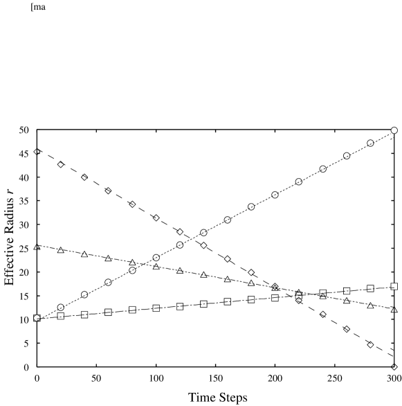
Figure 5: The evolution and contraction of the effective radii of the crystal nuclei and liquid voids calculated from (20) plotted as the function of time steps. $\square$: crystal nucleus when $\epsilon=0.1$, $\bigcirc$: crystal nucleus when $\epsilon=0.3$, $\triangle$: liquid void when $\epsilon=0.1$, $\lozenge$: liquid void when $\epsilon=0.3$. $q$ is set to $q=2$ for all four cases. The total area is 100$\times$100=10000 pixels. The straight lines are the least-square fittings to the numerical data.

The velocities $v$ estimated from Fig. 5 are summarized in Tab. 1. Table 1 shows that the analytical expression in eq.(18) gives a rough estimate of the front velocity. The velocity of shrinking void is always larger than the growing nucleus due to the capillary pressure as expected. Understanding that the cell dynamics method does not attempt to solve the original TDGL directly and, hence, is not guaranteed to reproduce the analytical expression (18), the discrepancy between the cell dynamics simulation and theoretical prediction in (18) seems not so serious. There is also a problem of the definition of the area $S$ of the growing phase, which will also numerically affect the front velocity calculated from (20).

Table 1: The front velocities of the growing new stable phase (nucleus) and shrinking unstable phase (void) obtained from the cell dynamics simulation of Fig. 5 compared with the theoretical prediction from eq.(18). The critical radii calculated from eq.(19) are also shown for reference.

$\epsilon$	$R_{c}$	$v$	$v_{\rm crystal-liquid}$	$v_{\rm crystal-liquid}$
	(Theoretical)	(Theoretical)	(growing)	(shrinking)
0.1	4.71	0.106	0.023	0.045
0.3	1.57	0.318	0.133	0.146

From the comparison of the cell dynamics simulation and the theoretical prediction from the TDGL for the two-phase system, we have confidence that this cell dynamics method should be effective to study the qualitative features of the evolution of the metastable phase in a three-phase system, which we will discuss in the next subsection of this paper. More details about the application of the cell dynamics method to the phase transformation in a two-phase system and the simulation of the so-called Kolmogorov-Johnson-Mehl-Avram (KJMA) kinetic will be presented elsewhere Iwamatsu and Nakamura .

III.2 Long-lived metastable phase in a three-phase system

Since we are most interested in the evolution or regression of the metastable phase during the phase transformation after nucleation, we will study the kinetics of phase transformation when three phases exist using the model free energy defined by eq.(9) and depicted in Fig. 1.

The phase diagram of this system which we will study is shown in Fig. 6. The equilibrium stable vapor phase has an order parameter $\psi_{v}=-1$ and the stable crystal phase has $\psi_{c}=1$, then the vapor-crystal coexistence lines (binodal) are the vertical lines at $\psi_{v}=-1$ and $\psi_{c}=1$. However, the stable liquid at $\psi_{l}=0$ exists only at the triple point $\epsilon_{t}=0$.

Once the stable liquid phase disappears from the equilibrium phase diagram when $\epsilon>0$, it can be considered to be hidden or buried as a metastable liquid phase within the vapor-crystal binodal. Even this metastable liquid cannot exist if $\epsilon>\epsilon_{c}$ where $\epsilon_{c}=0.5$. The hidden critical point is at $\epsilon_{c}=0.5$ and $\psi=0$, where the metastable liquid becomes completely unstable.

There are also hidden vapor-liquid and a liquid-crystal local coexistence lines (binodals), which are given by the co-tangency points $\psi_{v}^{{}^{\prime}}$ and $\psi_{l}^{{}^{\prime}}$ of the common tangent between the vapor and liquid free energy and by $\psi_{l}^{{}^{\prime\prime}}$ and $\psi_{c}^{{}^{\prime\prime}}$ between the liquid and crystals energy respectively. These hidden binodals disappear at $\epsilon=\epsilon_{m}$ with $\epsilon_{m}=0.2044$ where the solutions of the simultaneous equations, for example

$$h^{{}^{\prime}}\left(\psi_{l}^{{}^{\prime\prime}}\right) = h^{{}^{\prime}}\left(\psi_{c}^{{}^{\prime\prime}}\right)$$

$$h\left(\psi_{l}^{{}^{\prime\prime}}\right)-h^{{}^{\prime}}\left(\psi_{l}^{{}^{\prime\prime}}\right)\psi_{l}^{{}^{\prime\prime}} = h\left(\psi_{c}^{{}^{\prime\prime}}\right)-h^{{}^{\prime}}\left(\psi_{c}^{{}^{\prime\prime}}\right)\psi_{c}^{{}^{\prime\prime}}$$ (21)

ceases to exist, and the hidden binodal lines are terminated by the spinodal lines as shown in Fig. 6. Then, the vapor-liquid and the liquid-crystal coexistence could be established locally even when the liquid phase is metastable so long as $\epsilon<\epsilon_{m}$.

For the free energy (8), the spinodal lines are defined by the condition:

$$\frac{d^{2}h}{d\psi^{2}}=0$$ (22)

which gives the outer spinodal lines $\psi_{\rm sp1}$:

$$\psi_{\rm sp1}=\pm\sqrt{\frac{2}{5}-\frac{\epsilon}{5}+\frac{\sqrt{7-2\epsilon+3\epsilon^{2}}}{5\sqrt{3}}}$$ (23)

and inner spinodal lines $\psi_{\rm sp2}$:

$$\psi_{\rm sp2}=\pm\sqrt{\frac{2}{5}-\frac{\epsilon}{5}-\frac{\sqrt{7-2\epsilon+3\epsilon^{2}}}{5\sqrt{3}}}$$ (24)

The latter merge at $\psi_{l}=0$ and $\epsilon_{c}=0.5$. Therefore, the spinodal region consists of two regions sandwiched by an outer spinodal and an inner spinodal lines when $\epsilon<\epsilon_{c}$ while it consists of one region for $\epsilon>\epsilon_{c}$ as shown in Fig. 6.

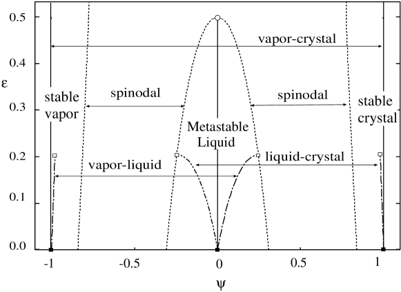
Figure 6: The phase diagram for the model triple-well free energy defined by (9). The model realizes the stable vapor and crystal phase at $\psi_{v}=-1$ (solid vertical line) and $\psi_{c}=1$ (solid vertical line) respectively and the metastable liquid phase at $\psi_{l}=0$ (solid vertical line) if $0<\epsilon<\epsilon_{c}$ with $\epsilon_{c}=0.5$. The triple point is at $\epsilon_{t}=0$ when three phases ($\blacksquare$) are all stable and can coexist. The metastable liquid ceases to exist at $\psi=0$ and $\epsilon_{c}=0.5$ which is the hidden critical point ($\bigcirc$). There are not only the vapor-crystal binodal (two vertical solid lines) but the hidden vapor-(metastable) liquid binodal (single-dot chain curve) and hidden (metastable)liquid-crystal binodal (double-dots chain curve), which can be constructed from the common tangent as shown in Fig. 1. These two pars of binodal disappear ($\square$) when they terminate the spinodal lines (dotted curves) at $\epsilon_{m}=0.2044$. The spinodal regions are also complex because of the existence of the metastable liquid phase.

We have incorporated the above free energy (9) into the cell-dynamics code Gaylord and Nishidate (1996) written by Mathematica TM Wolfram (2003). We have considered the growth of several special forms of circular nucleus which consist of two layers of two different phases embedded in another phase to see the possibility of the appearance of the long-lived metastable phase.

In figure 7 we start from the special structure where the stable vapor phase is wrapped by the metastable liquid layer, which is further embedded in a stable crystal. The initial crystal, liquid and vapor phases are prepared by randomly selecting the order parameter $\psi$ from 0.9 to 1.1 for crystal, from -0.3 to 0.3 for liquid and from -1.1 to -0.9 for vapor phases. From the analogy of the expansion of a stable nucleus and the shrinking of metastable inner void in a two-phase system, it is expected that the outermost crystal phase expands inward and the inner vapor core expands outward by consuming the intermediate metastable liquid layer. Actually, the crystal-liquid interface move inward as expected while the liquid-vapor interface does not move significantly. The vapor core does not move significantly even if the radius is larger than the critical radius as the surrounding metastable liquid layer has finite thickness, while the crystal-liquid front shrinks because no critical radius exists. As has been discussed in eq.(16), the capillary pressure accelerates the shrinking crystal-liquid interface, while it decelerates the growing liquid-vapor interface. Then, the slow liquid-vapor interface does not have enough time to move because metastable liquid is consumed by the fast crystal-liquid interface. Finally, the metastable liquid layer disappears completely and the stable vapor core is surrounded by the stable crystal phase and the vapor-crystal coexistence is established.

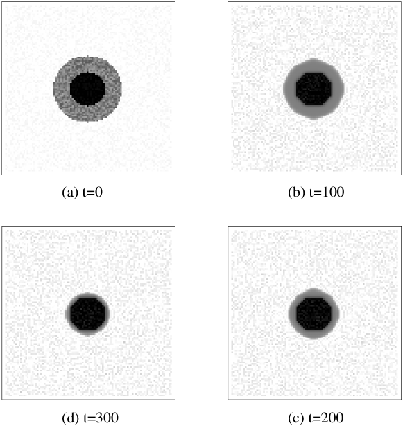
Figure 7: A Gray-level view of the dynamics of a three-layer nucleus when $\epsilon=0.1$. The black area is the vapor phase, the gray area is the metastable liquid phase, and the white area is the crystal phase. (a) Initial state is the stable vapor nucleus (black) wrapped by the metastable liquid layer (gray) which is further embedded in the stable crystal phase (white). (b), (c) the outer crystal-liquid interface shrinks inward by consuming the metastable liquid layer while the inner liquid-vapor interface does not expand significantly. (c) Finally the stable vapor phase is surrounded by the stable crystal phase and the vapor-crystal coexistence is established.

Figure 8 shows the time evolution of the effective radii of the crystal-liquid and the liquid-vapor interface estimated from the area of the nucleus from (20). We defined the area $S$ of three phases as the number of pixels which belong to them; the pixel of vapor is defined by the order parameter $\psi<-0.5$, that of crystal by $\psi>0.5$ and that of liquid by $-0.5\geq\psi\geq 0.5$. Figure 8 clearly indicates that the effective radius of the crystal-liquid interface decreases with constant velocity $v$ while that of the liquid-vapor interface remains almost constant. The crystal-liquid interfacial velocity estimated by fitting the straight line to the simulation result is $v=0.026$ which is again the same order of magnitude as the interfacial velocity in a two-phase system listed in Tab. 1.

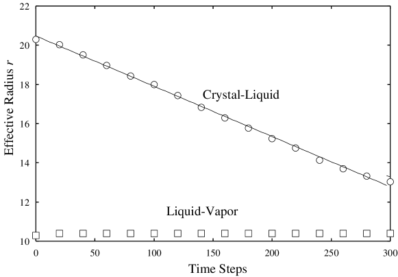
Figure 8: The time evolution of the effective radius of a circular crystal-liquid ($\bigcirc$) and liquid-vapor ($\square$) interface when $\epsilon=0.1$. The total area is 100$\times$100=10000. The radius of the crystal-liquid interface decreases while that of the liquid-vapor interface remains almost constant.

When the metastable liquid core is surrounded by the stable crystal and vapor phases, the crystal-liquid interface shrinks and the metastable liquid void disappears as shown in Fig. 9. The vapor-crystal interface does not move appreciably because the vapor and the crystal phases are in equilibrium and can coexist. Since our cellular dynamics model uses continuous order parameter $\psi$, the order parameter changes continuously in space. Then, there is always a thin layer of liquid with $\psi_{l}=0$ between the crystal core with $\psi_{c}=1$ and the vapor environment with $\psi_{v}=0$ in Fig. 9.

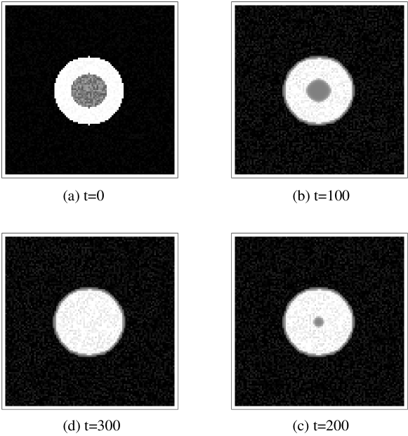
Figure 9: The same as figure 7 when $\epsilon=0.1$ but for the different ordering of the layers. (a) Initial state is the metastable liquid void (gray) wrapped by the stable crystal (white) layer which is further embedded in a stable vapor (black). (b), (c) the metastable liquid void shrinks while the outer stable crystal-vapor interface remains the same. (c)Finally the stable crystal phase is surrounded by the stable vapor phase and the vapor-crystal coexistence is established. There is always a thin layer of liquid at the solid-vapor interface because we use continuous order parameter $\psi$.

Figure 10 shows that the effective radius of the vapor-crystal interface remains constant while that of the crystal-liquid interface decreases almost linearly. The crystal-liquid interfacial velocity is estimated to be $v=0.023$ which is again comparable to the values shown in Tab. 1 for the two-phase system.

Figure 10: The time evolution of the effective radius of circular vapor-crystal ($\bigcirc$) and crystal-liquid ($\square$) interface when $\epsilon=0.1$. The radius of outer crystal-vapor interface remains the same while that of the crystal-liquid interface decreases.

These two examples have clearly indicated that the behavior of the stable core and the metastable void in a triple-phase system is similar to those in a two-phase system.

When the composition of the circular nucleus changes, a very interesting behavior is observed. In Figure 11, we start from the special structure where the stable circular crystal core is wrapped by a stable vapor layer, which is further embedded in a metastable liquid environment. The initial crystal, liquid and vapor phases are prepared by randomly selecting the order parameter $\psi$ from 0.9 to 1.1 for crystal, from -0.3 to 0.3 for liquid and from -1.1 to -0.9 for vapor phases respectively as before. Intuitively, we expect that the stable inner crystal core may not grow because of the crystal-liquid coexistence while the stable outer vapor layer expands outward by consuming the metastable liquid environment. However, we observe that this threefold structure is rather stable for a very long time. The crystal phase as well as the vapor phase cannot grow and the metastable liquid phase survives and occupies almost the same region for a long time as if the vapor-liquid coexistence is locally established at the liquid-vapor interface.

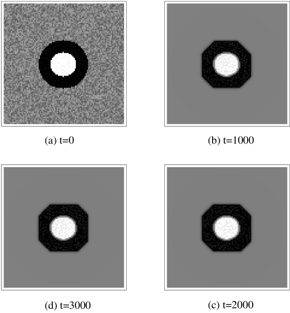
Figure 11: The Gray-level view of the dynamics of a three-layer nucleus when $\epsilon=0.1$. (a) Initial state is the stable crystal core (white) wrapped by the stable vapor (black) layer which is further embedded in the metastable liquid (gray). (b), (c), (d) The initial structure does not change appreciably even after very long time steps $t$=1000, 2000, 3000. Note the difference of time scale from Figs. 7 and 9. Again, there is always a thin layer of liquid at the solid-vapor interface as in Fig. 9.

Figure 12 shows the time evolution of the effective radius of the vapor-crystal and liquid-vapor interface estimated from the area of the nucleus calculated from (20). We confirm the stable vapor-crystal as well as the stable liquid-vapor interfaces which do not move appreciably. In order to confirm the numerical accuracy of Fig. 11, we check the evolution of a dual system where crystal and vapor is exchanged. Figure 13 clearly indicates that the dual system shows exactly the same behavior as in Fig. 11.

Figure 12: The time evolution of the effective radii of a circular vapor-crystal ($\square$) and liquid-vapor ($\bigcirc$) interface when $\epsilon=0.1$. The total area is 100$\times$100=10000. The two radii which remain almost constant indicating that the growth of stable core is prohibited and the long-lived liquid phase survives even though it is thermodynamically metastable. Note the long time scale compared with Figs. 8 and 10.

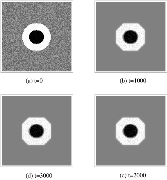
Figure 13: The same as Fig. 11, but now the stable vapor core (black) is wrapped by the stable crystal (white) layer which is further embedded in the metastable liquid (gray). We observe exactly the same morphology as in Fig. 11 if we exchange black (vapor) and white (crystal).

These striking results may be interpreted from the shape of the free energy in Fig. 1 using the argument of Cahn Cahn (1969). Since the parameter $\epsilon=0.1$, the system remains in the region of phase diagram (Fig. 6) where a hidden liquid-vapor binodal exists and we can draw a common tangent between the vapor and liquid phases. This means that it is possible to establish local liquid-vapor coexistence by changing the local pressure or the chemical potential even though the liquid phase is metastable (Fig. 1 ). Then, the liquid-vapor interface can not move. The faceted structure of the liquid-vapor interface appears probably due to the high symmetry of the problem since we put the nucleus at the center of the area and the nearest and the next-nearest neighbors are used to calculate the Laplacian. The flat interface is also favorable to mitigate the capillary pressure which acts to expand the liquid-vapor interface. A similar faceted structure appears also in the stable liquid-vapor interface in Fig. 7.

Furthermore, since this stable vapor layer is so tightly attracted by an inner crystal core to maintain vapor-crystal coexistence, the vapor-crystal interface also can not move. Therefore this special three-layer structure which Renth et al. Renth et al. (2001) called the ”boiled-egg crystal” becomes rather stable. The existence of this stable crystal wrapped by stable vapor layer in metastable liquid is predicted theoretically from the shape of the free energy Cahn (1969); Evans and Cates (1997); Renth et al. (2001) and suggested experimentally in a colloid-polymer mixture Poon (2002); Poon et al. (1999).

We note in passing, that this boiled-egg crystal is in sharp contrast to the transient metastable phase predicted from the steady state solution of the Ginzburg-Landau equation. This transient phase appears when it is sandwiched by the two stable phase due to the difference of the front speed of two interfaces of the stable and metastable phase Evans and Cates (1997); Bechhoefer et al. (1991); Celestini and ten Bosh (1994), while our long-lived metastable phase appears when it surrounds the two stable phases.

As the parameter $\epsilon$ increases further above 0.2, the hidden liquid-vapor coexistence cannot be established (Fig. 1), because we cannot construct a common tangent. Then this boiled-egg crystal structure cannot remain stable as shown in Fig. 14. The vapor phase starts to grow by consuming the metastable liquid phase, while core crystal phase remains almost the same size and the shape. Finally the metastable liquid phase disappears and the stable crystal phase is wrapped by the stable vapor phases and the vapor-crystal coexistence is established. Here again, the initial crystal, liquid and vapor phases are prepared by randomly selecting the order parameter $\psi$ from 0.9 to 1.1 for crystal, from -0.3 to 0.3 for liquid and from -1.1 to -0.9 for vapor phases.

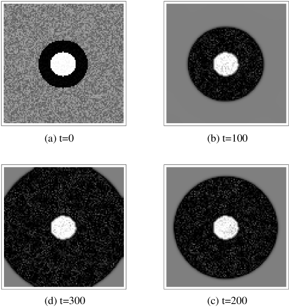
Figure 14: The same as Fig. 11 when $\epsilon=0.3$. (a) Initial state is the stable crystal core (white) wrapped by the stable vapor layer (black) which is further embedded in the metastable liquid. (b), (c) The stable vapor layer grows by consuming the metastable liquid environment, while the stable crystal core remains the same. (c) Finally the stable crystal phase is surrounded by the stable vapor phase and the vapor-crystal coexistence is established.

Figure 15 clearly indicates that the effective radius of the liquid-vapor interface increases while that of the vapor-crystal interface remains the same as the function of time. The liquid-vapor interfacial velocity estimated by fitting the straight line to the simulation data is $v=0.112$ which is the same order of magnitude listed in Tab. 1 for the two-phase system.

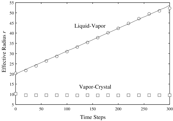
Figure 15: The time evolution of the effective radii of the circular vapor-crystal ($\square$) and liquid-vapor ($\bigcirc$) interfaces. The total area is 100$\times$100=10000. The radius of liquid-vapor interface increases linearly while that of the vapor-crystal interface remains almost constant as the function of time.

Similarly, this long-lived boiled-egg structure will be destroyed by the thermal noise, which can be simulated by using the cell dynamics equation Puri and Oono (1988)

$$\psi(t+1,n)=F[\psi(t,n)]+B\eta(t,n)$$ (25)

instead of (4), where $B$ is the amplitude of the noise, $\eta(t,n)$ is a uniform random number between -1.0 and 1.0.

In Fig. 16, we start from the same special structure as in Fig. 11 when $\epsilon=0.1$ but the thermal noise with $B=0.07$ is included. The thermal noise certainly destroys the long-lived metastable configuration as expected, but it still remains rather stable for a long time. The thermal noise also destroys the circular or even the faceted structure and the liquid-vapor interface becomes flat. The thermal noise acts to eliminate the curvature of the interface to suppress the capillary pressure.

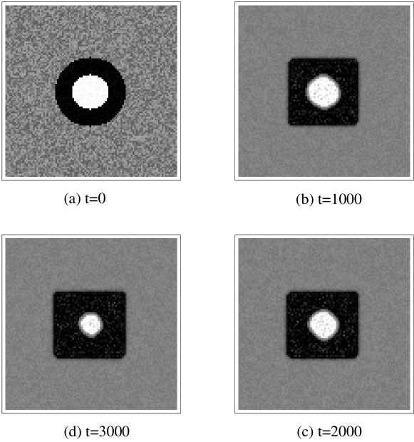
Figure 16: The same as Fig. 11 but the thermal noise with $B=0.07$ is included. The long-lived metastable state is destroyed by the thermal noise, however the structure is still rather stable for a long time.

Naturally, the larger the thermal noise, the shorter the lifetime of the metastable configuration as shown in Fig. 17. A similar effect of noise on the time-scale of the evolution was observed in the TDGL model of nucleation Valls and Mazenko (1990) for a non-conserved order parameter.

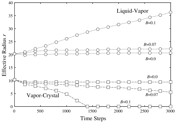
Figure 17: The same as Fig. 12 for various noise lever $B=0.00$ (Fig. 12), $B=0.07$, and $B=0.1$ when $\epsilon=0.1$. The effective radius of the liquid-vapor interface starts to increases and that of the vapor-crystal interface starts to decrease as we increase the noise level $B$. However, the time scale is still much longer than Fig. 15.

These last four examples indicate that the kinetics of phase transformation is definitely affected by the presence of metastable phase and the hidden binodals which is in no way related to the equilibrium phase diagrams. The long-lived metastable phase could appear macroscopically if it accommodates the special composite nucleus which consists of a stable crystal core surrounded by an equally stable vapor layer.

IV Conclusion

In this paper, we have used the cell-dynamics method to study the evolution of a single composite nucleus. We have studied the three-phase system which has a hidden binodal with two stable and one metastable phases. We have called two stable phases, crystal and vapor, and one metastable phase liquid. We could successfully simulate the evolution of stable phases and the regression of metastable phase. We have found, however, one special configuration of a stable crystal core wrapped by a stable vapor layer embedded in the metastable liquid environment becomes stable and stationary for long time. This means that the long-lived metastable environment phase can persist and can appear as a macroscopic phase even though it is thermodynamically metastable. According to the argument of Cahn Cahn (1969), this result can be interpreted from the hidden liquid-vapor binodal which can be constructed from the common tangent between the stable vapor and metastable liquid phases.

In conclusion, we have used a cell dynamics method to study the growth of a single nucleus which has traditionally been explained using the partial differential equation derived from time-dependent-Ginzburg-Landau equation Valls and Mazenko (1990) or the so-called phase field model Castro (2003); Gránásy et al. (2004). We have found that the long-lived metastable phase can appear during the phase transformation as predicted by several researchers Ostwald (1897); Cahn (1969); Poon (2002); Renth et al. (2001). This cell-dynamics method is not only flexible but numerically stable to handle such a complex situation when many phases can coexist. Further extension and modification of the method to explain the formation of various intermediate phases will be possible.