Multiple scattering formalism for correlated systems: A KKR+DMFT approach

Abstract

We present a charge and self-energy self-consistent computational scheme for correlated systems based on the Korringa-Kohn-Rostoker (KKR) multiple scattering theory with the many-body effects described by the means of dynamical mean field theory (DMFT). The corresponding local multi-orbital and energy dependent self-energy is included into the set of radial differential equations for the single-site wave functions. The KKR Green’s function is written in terms of the multiple scattering path operator, the later one being evaluated using the single-site solution for the $t$-matrix that in turn is determined by the wave functions. An appealing feature of this approach is that it allows to consider local quantum and disorder fluctuations on the same footing. Within the Coherent Potential Approximation (CPA) the correlated atoms are placed into a combined effective medium determined by the dynamical mean field theory (DMFT) self-consistency condition. Results of corresponding calculations for pure Fe, Ni and Fe_xNi_1-x alloys are presented.

I Introduction

One of the first band structure methods formulated in terms of Green’s functions is the KKR method of Koringa, Kohn and Rostoker Kor47 ; KR54 . Although it is not counted among the fastest band structure methods, it is usually regarded as a very accurate technique. The advantage of the KKR method lies in the transparent multiple scattering formalism which allows to express the Green’s function in terms of single-site scattering and geometrical or structural quantities. A second outstanding feature of the KKR method is the Dyson equation relating the Green’s function of a perturbed system with the Green’s function of the corresponding unperturbed reference system. Because of this property, the KKR Green’s function method allows to deal with substitutional disorder including both diluted impurities and concentrated alloys in the framework of the Coherent Potential Approximation (CPA) Fau82 . Within this approach (KKR-CPA) the propagation of an electron in an alloy is regarded as a succession of elementary scattering processes due to random atomic scatterers, with an average taken over all configurations of the atoms. This problem can be solved assuming that a given scattering center is embedded in an effective medium whose choice is open and can be made in a self-consistent way. The physical condition corresponding to the CPA is simply that a single scatterer embedded in the effective CPA medium should produce no further scattering on the average. A similar philosophy is applied also when dealing with many-body problems for crystals in the framework of the so called dynamical mean field theory (DMFT, for review see Ref. GKKR96, ). Thus it seems to be rather natural to combine the DMFT and KKR methods to arrive at a very reliable and flexible band structure scheme that include correlation effects beyond the standard local density (LDA) or generalized (GGA) approximations. In fact the combination of the KKR-CPA for disordered alloys and the DMFT scheme is based on the same arguments as used by Drchal et al.DJK99 when combining the TB-LMTO Green’s function method for alloys TDK+97 with the DMFT. In contrast to their approach, however, the formalism presented below allows to incorporate correlation effects via a corresponding self-energy when calculating the electronic single-site wave functions.

First attempts to achieve a self-consistent description of local correlation effects in crystals have been made already many years ago. In the third paper of a famous series Hubbard Hub64 has introduced an alloy analogy and by an appropriate decoupling scheme for the Green’s function a set of equations has been derived that represent a self-consistent formulation equivalent to the CPA approximation. In contrast to the DMFT the “Hubbard III” approximation considers quantum on-site fluctuations as static ones which leads to some shortcomings such as violation of some Fermi liquid properties, missing of the so called Kondo peak near the metal-insulator transition GKKR96 . Keeping in mind the above conceptual analogies it is our purpose to present here a combined Local Density Approximation and Dynamical Mean Field Theory (LDA+DMFT) electronic structure technique, including the case of disordered solids, in the framework of the KKR method. The many-body correlation effects are treated by means of the DMFT, while the disorder is described in the framework of the CPA. Taking into account the local nature of the DMFT approximation the self-energy is represented by a local complex energy dependent quantity (which is a matrix in orbital indices) viewed as a contribution to the electronic potential. We note that for a general non-local energy dependent potential multiple scattering theory offers a solution known as the optical potential Tay83 . However, the nonlocal self-energy is far too complicated to be used in a realistic computation.

Very recently a combined LDA+DMFT computational scheme was proposed in which the so called Exact Muffin-tin band structure method was used. In the EMTO approach AJK94 ; AS00 ; VSJ+00 the one-electron effective potential is represented by the optimized overlapping muffin-tin potential which is considered as the best possible spherical approximation to the full-one electron potential. In essence the one-electron Green’s function is evaluated on a complex contour similarly to the screened KKR technique, from which it was derived. In the iteration procedure the LDA+DMFT Green’s function is used to calculate the charge and spin densities. Finally, for the charge self-consistent calculation one constructs the new LDA effective potential from the spin and charge densities CVA+03 , using the Poisson equation in the spherical cell approximation Vit01 .

In contrast to the EMTO implementation CVA+03 , the present work follows a natural development in which the self-energy is added directly to the coupled radial differential equations which determine the electronic wave function within a potential well and this way the single-site $t$-matrix. Because this way also the scattering path operator of multiple scattering theory used to set up the electronic Green’s function is determined unambiguously, no further approximations are needed to achieve charge self-consistency.

The paper is organized as follows. Section II presents a general formulation of the problem. Section II.1 provides an extension of the derivation of the multiple scattering Green’s function to include the self-energy, and in particular provides the information on the many-body solver. Section II.2 describes the many-body solver used in our calculation, that is based on a modified fluctuating exchange interaction approximation. The combined self-consistency cycle is presented in section II.4. Finally, results and discussions are presented in section III.

II Formulation of the problem

The DMFT method has already been implemented within several band structure methods based on a wave function formalism: first in the linear muffin-tin orbital method in atomic sphere approximation (ASA-LMTO) APK+97 ; LK98 ; KL99 and then in full-potential LMTO SKA01 ; SK04 , as well as in a screened KKR or exact muffin-tin orbitals approach (EMTO)CVA+03 . The emerged LDA+DMFT method can be used for calculating the electronic structure for a large variety of systems with different strength of the electronic correlations (for a review, see Refs. LKK02, ; HNK+02, ). To underline the importance of complete LDA+DMFT self-consistency we mention that the first successful attempt to combine the DMFT with LDA charge self-consistency gave an important insight into a long-standing problem of phase diagram and localization in f-electron systems SKA01 ; SK04 and has been used also to describe correlation effects in half-metallic ferromagnetic materials like NiMnSb CKG+03 . As an alternative to the above mentioned band structure methods, accurate self-consistent methods for solving the local Kohn-Sham equations based on LDA in terms of Green’s functions have been developed within the multiple scattering theory (KKR-method) Gyo72 ; Ric84 ; FS80 ; Wei90 . For that reason the KKR-method can be combined, as it will be shown below, in a natural way with the LDA+DMFT approach. A further appealing feature of this scheme is that the CPA alloy theory can also be incorporated very easily.

In order to account within LDA-band structure calculations for correlations an improved hybrid Hamiltonian was proposed by Anisimov et al.AZA91 ; AAL97 . In its most general form such a Hamiltonian is written as

$$H=H_{LDA}+H_{U}-H_{DC}\;,$$ (1)

where $H_{LDA}$ stands for the ordinary LDA Hamiltonian, $H_{U}$ describes the effective electron-electron interaction and the one-particle Hamiltonian $H_{DC}$ serves to eliminate double counting of the interactions already accounted for by $H_{LDA}$.

Using second quantization a rather general expression for $H_{U}$ is given by:

$$H_{U}=\frac{1}{2}\sum_{n,ijkl}U^{n}_{ijkl}\hat{C}^{\dagger}_{ni}\hat{C}^{\dagger}_{nj}\hat{C}_{nk}\hat{C}_{nl}\;,$$ (2)

where $n$ runs over all the sites of the crystal $\vec{R}_{n}$ and the creation ($\hat{C}^{\dagger}$) and annihilation ($\hat{C}$) operators are defined with respect to some subset of localized orbitals $\phi_{i}(\vec{r}-\vec{R}_{n})$. The constants $U^{n}_{ijkl}$ are matrix elements of the screened Coulomb interaction $v(\vec{r}-\vec{r}\,^{\prime})$:

$$U^{n}_{ijkl}=\int\phi^{\dagger}_{i}(\vec{r}-\vec{R}_{n})\phi^{\dagger}_{j}(\vec{r}\,^{\prime}-\vec{R}_{n})v(\vec{r}-\vec{r}\,^{\prime})\phi_{k}(\vec{r}\,^{\prime}-\vec{R}_{n})\phi_{l}(\vec{r}-\vec{R}_{n})d\vec{r}d\vec{r}\,^{\prime}\;.$$ (3)

The resulting many-particle Hamiltonian can not be diagonalized exactly, thus various methods were developed in the past to find an approximate solution GKKR96 . Among them one of the most promising approaches is to solve Eq. (1) within dynamical mean field theory, a method developed originally to deal with the Hubbard model.

The main idea of DMFT is to map a periodic many-body problem onto an effective single-impurity problem that has to be solved self-consistently. For this purpose one describes the electronic properties of the system in terms of the one particle Green’s function $\hat{G}(E)$, being the solution of the equation:

$$(E-\hat{H}-\hat{\Sigma}(E))\hat{G}=\hat{1}\;,$$ (4)

where $E$ is the complex energy and the effective self-energy operator $\hat{\Sigma}$ is assumed to be a single-site quantity for site $n$:

$$\hat{\Sigma}(E)=\sum_{ij}|\phi_{ni}\rangle\Sigma_{ij}(E)\langle\phi_{nj}|\;.$$ (5)

Within DMFT, the self-energy matrix $\Sigma_{ij}(E)$ is a solution of the many-body problem of an impurity placed in an effective medium. This medium is described by the so called bath Green’s function matrix $\mathcal{G}$ defined as:

$$\mathcal{G}_{ij}^{-1}(E)=G_{ij}^{-1}(E)+\Sigma_{ij}(E)\;,$$ (6)

where $G_{ij}(E)$ is calculated as a projection of $\hat{G}(E)$ onto the impurity site:

$$G_{ij}(E)=\langle\phi_{ni}|\hat{G}(E)|\phi_{nj}\rangle\;.$$ (7)

As the self-energy $\Sigma_{ij}(E)$ depends on the bath Green’s function $\mathcal{G}_{ij}(E)$ the DMFT equations have to be solved self-consistently. Accordingly, from a technical point of view the problem can be split into two parts. One is dealing with the solution of Eq. (4) and the second one is the effective many-body problem to find the self-energy $\Sigma_{ij}(E)$. Within the present work, the first task is solved by the KKR band structure method, as described below in Sec. II.1. The details of solving the many-body effective impurity problem based on the fluctuation exchange (FLEX) approximation BS89a will be presented in Sec. II.2.

II.1 The KKR+DMFT formalism

In this section we present an extension of the well known KKR equations in order to include the local, multi-orbital and energy dependent self-energy produced by the many-body solver (see section II.2). In the framework of the multiple scattering formalism the solution of Eq. (4) is constructed in two steps. For the first step one has to solve the so called single-site scattering problem, to obtain the regular ($Z$) and irregular solution ($J$) of the corresponding Schrödinger (or in our case Lippmann-Schwinger) equations as well as a scattering amplitude expressed in terms of the single-site $t$-matrix.

II.1.1 Solution of the single-site problem

The solution of the single-site problem can be worked out easily in the same way as in the full-potential description Zel87a . This way one finally gets the single-site $t$-matrix for the LDA+DMFT case. In terms of the wave functions the single-site quasiparticle equation to be solved for each spin channel $\sigma$ reads

$$[-\nabla^{2}+V^{\sigma}(r)-E]\Psi(\vec{r})+\int\Sigma^{\sigma}(\vec{r},\vec{r}\,^{\prime},E)\Psi(\vec{r}\,^{\prime})d^{3}r\,^{\prime}=0.$$ (8)

In the following we omit the spin index $\sigma$ for the moment keeping in mind that for a spin-polarized system described in a non-relativistic way one has to solve Eq. (8) for each spin channel independently. For the solution $\Psi_{\nu}(\vec{r})$ one can start from the ansatz:

$$\Psi_{\nu}(\vec{r})=\sum_{L}\Psi_{L\nu}(\vec{r})\;,$$ (9)

where the partial waves $\Psi_{L\nu}(\vec{r})$ are chosen to have the same form as the linearly independent solutions for the spherically symmetric potential:

$$\Psi_{L\nu}(\vec{r})=\Psi_{L\nu}(r)Y_{L}(\hat{r})\;,$$ (10)

with $L=(l,m_{l})$ standing for the angular momentum and magnetic quantum numbers and $Y_{L}(\hat{r})$ are spherical harmonics. Inserting the ansatz (9) into the single-site equation (8) and integrating over angle variables leads to the following set of the coupled radial integro-differential equations:

$$\left[\frac{d^{2}}{dr^{2}}-\frac{l(l+1)}{r^{2}}-V(r)+E\right]\Psi_{L\nu}(r,E)=\sum_{L^{\prime\prime}}\>\int r^{\prime 2}dr^{\prime}\Sigma_{LL^{\prime\prime}}(E)\>\phi_{l}(r)\phi_{l^{\prime\prime}}(r^{\prime})\Psi_{L\nu}(r^{\prime},E)\;,$$ (11)

For a general non-diagonal self-energy a similar radial equation (11) shall be written for the left-hand side equation. If one makes a rather natural choice of the localized subset of functions being just $\phi_{L}(\vec{r})=\phi_{l}(r)Y_{L}(\hat{r})$ (see below). In principle these equations can be solved by summing a corresponding Born series. In this work, however, we simplified the equations taking advantage of the following special representation for the self-energy:

$$\int d^{3}r^{\prime}\Sigma(\vec{r},\vec{r}\;^{\prime},E)\psi_{L}(\vec{r}\;^{\prime},E)=\sum_{L}\int d^{3}r^{\prime}\Sigma_{L^{\prime}L}(E)\phi_{L^{\prime}}^{\dagger}(\vec{r})\phi_{L}(\vec{r}\;^{\prime})\psi_{L}(\vec{r}\;^{\prime},E)\approx\sum_{L}\Sigma_{L^{\prime}L}(E)\psi_{L}(\vec{r},E)\;.$$ (12)

This way the Eq. (11) becomes a pure differential equation:

$$\left[\frac{d^{2}}{dr^{2}}-\frac{l(l+1)}{r^{2}}-V(r)+E\right]\Psi_{L\nu}(r,E)=\sum_{L^{\prime}}\>\Sigma_{LL^{\prime}}(E)\>\Psi_{L^{\prime}\nu}(r,E)\;.$$ (13)

After having solved the set of coupled equations for the wave functions one gets the corresponding single-site $t$-matrix by introducing the auxiliary matrices $a$ and $b$ Fau82 :

$$a_{L\nu}(E)=-ipr^{2}[h^{-}_{L}(pr),\Psi_{L}^{\nu}(r)]_{r}$$ (14)

$$b_{L\nu}(E)=-ipr^{2}[h^{+}_{L}(pr),\Psi_{L}^{\nu}(r)]_{r}\;.$$

Here $p=\sqrt{E}$ is the momentum, $h^{\pm}_{L}(pr)$ are Hankel functions of the first and second kind and $[\ldots]_{r}$ denotes the Wronskian. Evaluating the Wronskians at Wigner-Seitz radii $r_{WS}$ one finally has Fau82 ; EG88 :

$$t(E)=\frac{i}{2p}(a(E)-b(E))b^{-1}(E)\;.$$ (15)

The regular wave functions $Z$ used to set up the electronic Green’s function within the KKR-formalism FS80 are obtained by a superposition of the wave functions $\Psi_{\nu}$ according to the boundary conditions at $r=r_{WS}$:

$$Z_{L}(\vec{r},E)=\sum_{\nu}C_{L}^{\nu}\Psi_{\nu}(\vec{r})\stackrel{{\scriptstyle r=r_{WS}}}{{\longrightarrow}}\sum_{L\,^{\prime}}j_{L\,^{\prime}}(\vec{r},E)t(E)^{-1}_{L,L\,^{\prime}}-iph^{+}_{L}(\vec{r},E)\;,$$ (16)

The irregular solutions $J_{L}$ needed in addition are fixed by the boundary condition

$$J_{L}(\vec{r},E)\stackrel{{\scriptstyle r=r_{WS}}}{{\longrightarrow}}j_{L}(\vec{r},E)$$ (17)

and are obtained just by inward integration with the functions $j_{L}$ being the spherical Bessel functions.

II.1.2 The multiple scattering Green’s function

Having constructed a set of regular ($Z$) and irregular ($J$) solutions of the single-site problem together with the $t$-matrix the corresponding expression for the Green’s function reads FS80 :

$$G(\vec{r}_{n}+\vec{R}_{n},\vec{r}^{\;\prime}_{m}+\vec{R}_{m},E) = \sum_{L,L^{\prime}}Z_{L}(\vec{r}_{n},E)\tau^{nm}_{L,L^{\prime}}(E)Z^{\times}_{L^{\prime}}(\vec{r}^{\;\prime}_{m},E)\;$$ (18)

$$- \delta_{nm}\sum_{L}\{Z_{L}(\vec{r}_{n},E)J^{\times}_{L}(\vec{r}^{\;\prime}_{n},E)\Theta(r^{\;\prime}_{n}-r_{n})$$

$$+ J_{L}(\vec{r}_{n},E)Z^{\times}_{L}(\vec{r}^{\;\prime}_{n},E)\Theta(r_{n}-r^{\;\prime}_{n})\}\;.$$

Here the superscript $\times$ is used to distinguish between the left and right hand solutions to Eq. (8); i.e. for example $|Z>$ and $<Z^{\times}|$ are solutions to the adjoint equations Tam92 :

$$(\hat{H}+\hat{\Sigma}-E)|Z\rangle = 0$$ (19)

$$\langle Z^{\times}|(\hat{H}+\hat{\Sigma}-E) = 0\;.$$ (20)

The central quantity in Eq. (18) is the scattering path operator $\tau$ which for the case of a periodic crystal can be obtained from the Brillouin zone (BZ) integration:

$$\tau^{nm}_{LL^{\prime}}(E)=\frac{1}{V_{\rm BZ}}\int_{V_{\rm BZ}}{\rm d}^{3}k\left[t^{-1}(E)-G(\vec{k},E)\right]^{-1}_{L^{\prime}L}e^{i\vec{k}\vec{R}_{nm}}\ ,$$ (21)

where $V_{\rm BZ}$ is the volume of the first Brillouin–zone and $\vec{R}_{nm}=\vec{R}_{n}-\vec{R}_{m}$ with $\vec{R}_{n(m)}$ denoting the lattice vector specifying the position of the unit cell $n(m)$ and the matrix $t^{-1}(E)-G(\vec{k},E)$ occurring in the integral is known as the KKR matrix. The matrix $G(\vec{k},E)$ is the Fourier transform of the real space KKR structure constant matrix that depends only on the relative positions of scatterers.

Given the local nature of the many-body solver used within the DMFT approach, the KKR Green’s function (18) has to be projected accordingly to the matrix $G^{nm}_{LL\;\prime}$ (see Eq. (7)). The projection is performed through the following integration:

$$G^{nm}_{L,L^{\prime}}(E)=\sum_{L_{1},L_{2}}\left(\int d^{3}r_{1}\phi^{\dagger}_{L}({\bf r_{1}})Z_{L_{1}}({\bf r_{1}},E)\right)\tau^{nm}_{LL^{\prime}}(E)\left(\int d^{3}r_{2}Z_{L_{2}}^{\times}({\bf r_{2}},E)\phi_{L\;\prime}({\bf r_{2}})\right)$$

$$-\delta_{nm}\sum_{L_{1}}(\int d^{3}r_{2}\left(\int_{0}^{r_{2}}d^{3}r_{1}\phi^{\dagger}_{L}({\bf r_{1}})Z_{L_{1}}({\bf r_{1}},E)\right)J^{\times}_{L_{1}}({\bf r_{2}},E)\phi_{L^{\prime}}({\bf r_{2}})$$

$$+\int d^{3}r_{2}\left(\int_{r_{2}}^{r_{ws}}d^{3}r_{1}\phi^{\dagger}_{L}({\bf r_{1}})J_{L_{1}}({\bf r_{1}},E)\right)Z^{\times}_{L_{1}}({\bf r_{2}},E)\phi_{L^{\prime}}({\bf r_{2}}))\;.$$ (22)

The impurity Green’s function $G^{nm}_{LL^{\prime}}(E)$ (actually $G^{\sigma nm}_{LL^{\prime}}(E)$ for both spin channels) represents the input into the solution of the effective impurity problem presented below. As the DMFT-approach (see next section) concentrates on the correlation among electrons of the same angular momentum $l$ only the $l-l$-subblock of this matrix will be used in the following. For the transition metal systems dealt here this implies that only the $d-d$-subblock is considered with $\phi_{L}(\vec{r})$ being appropriate reference wave functions with $l=2$.

II.2 Solution of the effective impurity problem

Our approach to achieve a solution of the many-body effective impurity problem is based on the fluctuation exchange (FLEX) approximation BS89a but with a different treatment of particle-hole and particle-particle channels. The particle-particle channel is described by a $T$-matrix approach Gal58 ; Kan63 giving a renormalization of the effective interaction, the latter one being used explicitly in the particle-hole channel KL99 ; KL02 .

The symmetrization of the bare U matrix is done over particle-hole and particle-particle channels:

$$U^{d}_{m_{1}m_{3}m_{2}m_{4}} = 2U_{m_{1}m_{2}m_{4}m_{3}}^{i}-U_{m_{1}m_{2}m_{3}m_{4}}^{i}$$

$$U^{m}_{m_{1}m_{3}m_{2}m_{4}} = -U_{m_{1}m_{2}m_{3}m_{4}}^{i}$$

$$U^{s}_{m_{1}m_{3}m_{2}m_{4}} = \frac{1}{2}(U_{m_{1}m_{3}m_{2}m_{4}}^{i}+U_{m_{1}m_{3}m_{4}m_{2}}^{i})$$

$$U^{t}_{m_{1}m_{3}m_{4}m_{2}} = \frac{1}{2}(U_{m_{1}m_{3}m_{2}m_{4}}^{i}-U_{m_{1}m_{3}m_{4}m_{2}}^{i})\;.$$

As indicated above, here and in the following only matrix elements with respect to the $d$-like reference wave functions $\phi_{L}$ have to be considered. The above expressions are the matrix elements of bare interaction which can be obtained with the help of the pairwise operators corresponding to different channels:

• particle-hole density

  $$d_{12}=\frac{1}{\sqrt{2}}(c_{1\uparrow}^{+}c_{2\uparrow}+c_{1\downarrow}^{+}c_{2\downarrow})$$ (23)

• particle-hole magnetic

  $$m_{12}^{0} = \frac{1}{\sqrt{2}}(c_{1\uparrow}^{+}c_{2\uparrow}-c_{1\downarrow}^{+}c_{2\downarrow})$$

  $$m_{12}^{+} = c_{1\uparrow}^{+}c_{2\downarrow}$$ (24)

  $$m_{12}^{-} = c_{1\downarrow}^{+}c_{2\uparrow}$$

• particle-particle singlet

  $$s_{12} = \frac{1}{\sqrt{2}}(c_{1\downarrow}c_{2\uparrow}-c_{1\uparrow}c_{2\downarrow})$$

  $$\overline{s}_{12} = \frac{1}{\sqrt{2}}(c_{1\uparrow}^{+}c_{2\downarrow}^{+}-c_{1\downarrow}^{+}c_{2\uparrow}^{+})$$ (25)

• particle-particle triplet

  $$t_{12}^{0} = \frac{1}{\sqrt{2}}(c_{1\downarrow}c_{2\uparrow}+c_{1\uparrow}c_{2\downarrow})$$

  $$\overline{t}_{12}^{0} = \frac{1}{\sqrt{2}}(c_{1\uparrow}^{+}c_{2\downarrow}^{+}+c_{1\downarrow}^{+}c_{2\uparrow}^{+})$$

  $$t_{12}^{\pm} = c_{1\uparrow,\downarrow}c_{2\downarrow,\uparrow}$$

  $$\overline{t}_{12}^{\pm} = c_{1\uparrow,\downarrow}^{+}c_{2\downarrow,\uparrow}^{+}\;.$$ (26)

These operators describe the correlated movement of the electrons and holes below and above the Fermi level and play an important role in defining the spin-dependent effective potentials $W_{m_{1}m_{2}m_{3}m_{4}}^{\sigma\sigma^{\;\prime}}$. The one-electron Green’s function matrix containing the many-body interaction, described by the self-energy $\Sigma_{mm^{\;\prime}\sigma}(i\omega_{n})$ is given by the Dyson equation

$$\mathcal{G}_{mm^{\;\prime}\sigma}^{-1}(i\omega_{n})=(i\omega_{n}+\mu)\delta_{mm^{\;\prime}}-h_{mm^{\;\prime}\sigma}-\Sigma_{mm^{\;\prime}\sigma}(i\omega_{n})$$ (27)

where $\mu$ is the chemical potential, $\omega_{n}=(2n+1)\pi/\beta$ are Matsubara frequencies and $\beta=1/T$ is the inverse temperature. The GW type of diagrams are summed up self-consistently to produce the self-energy. For getting the self-energy we use a two-step FLEX approximation. This means that first of all the bare matrix vertex is replaced by the $T$-matrix approach Gal58 ; Kan63 which will be used in the calculation of the particle-hole channel. In the Kanamori $T$-matrix approach the sum over the ladder graphs may be carried out with the aid of the so called $T$-matrix which obeys the Dyson-like integral equation:

$$<13|T^{\sigma\sigma^{\;\prime}}(i\Omega)|24> =$$

$$<13|v|24> - \frac{1}{\beta}\sum_{\omega}\sum_{5678}<13|v|57>\mathcal{G}_{56}^{\sigma}(i\omega)\mathcal{G}_{78}^{\sigma^{\;\prime}}(i\Omega-i\omega)<68|T^{\sigma\sigma^{\;\prime}}(i\Omega)|24>\;.$$

The Hartree and Fock contribution are obtained replacing the bare interaction by a T-matrix:

$$\Sigma_{12,\sigma}^{(TH)}(i\omega) = \frac{1}{\beta}\sum_{\Omega}\sum_{34\sigma^{\prime}}<13|T^{\sigma\sigma^{\prime}}(i\Omega)|24>\mathcal{G}_{43}^{\sigma^{\prime}}(i\Omega-i\omega)$$ (28)

$$\Sigma_{12,\sigma}^{(TF)}(i\omega) = -\frac{1}{\beta}\sum_{\Omega}\sum_{34}<14|T^{\sigma\sigma}(i\Omega)|32>\mathcal{G}_{34}^{\sigma}(i\Omega-i\omega)\ .$$ (29)

In the low-density limit the self-energy should be the summation over diagrams for repulsion of two holes below $E_{F}$ (ladder approximation). Going beyond the low density limit means the inclusion of excitations of electrons from states below the Fermi level into the unoccupied part of the $d$ band. This process renormalizes the hole states below $E_{F}$ and put new poles for the Green’s function.

Combining the density and the magnetic parts of the particle-hole channel we can write the expression for the interaction part of the Hamiltonian KL99 ; KL02 :

$$H_{U} = \frac{1}{2}Tr(D^{+}*V^{\|}*D+m^{+}*V_{m}^{\bot}*m^{-}+m^{-}*V_{m}^{\bot}*m^{+})\;,$$ (30)

where $D$ is a row matrix with elements $(d,m^{0})$, and $D^{+}$ is a column matrix with elements $(d^{+}m_{0}^{+})$. We denote by * matrix multiplication with respect to the pairs of orbital indices. The expression for the effective potential is:

$$V^{\|}(i\omega) = \frac{1}{2}\left(\begin{array}[]{cc}{V}^{dd}&{V}^{dm}\\ {V}^{md}&{V}^{mm}\end{array}\right)$$ (33)

$$(V_{m}^{\bot})_{1234} = <13|T^{\uparrow\downarrow}|42>\;.$$ (34)

The matrix elements of the effective interaction for $z$ or longitudinal spin-fluctuations are:

$$V_{dd} = \frac{1}{2}\sum_{\sigma}(\sum_{\sigma^{\;\prime}}<13|T^{\sigma\sigma^{\;\prime}}|42>-<13|T^{\sigma^{\;\prime}\sigma^{\;\prime}}|42>)$$

$$V_{dm}=V_{md} = \frac{1}{2}\sum_{\sigma\sigma^{\;\prime}}\sigma(<13|T^{\sigma\sigma}|42>-<13|T^{\sigma\sigma}|24>+<13|T^{\sigma^{\;\prime}\sigma}|42>)$$

$$V_{mm} = \frac{1}{2}\sum_{\sigma}(\sum_{\sigma^{\;\prime}}\sigma\sigma^{\;\prime}<13|T^{\sigma\sigma^{\;\prime}}|42>-<13|T^{\sigma^{\;\prime}\sigma^{\;\prime}}|42>)\;.$$

For finite temperature the definition for the spin dependent Green’s function is:

$$\mathcal{G}_{12}^{\sigma}(\tau) = -<T_{\tau}c_{1\sigma}(\tau)c_{2\sigma}^{+}(0)>$$

$$\mathcal{G}_{12}^{\sigma}(i\omega_{n}) = \int_{0}^{\beta}e^{i\omega_{n}\tau}\mathcal{G}_{12}^{\sigma}(\tau)d\tau\;.$$

The corresponding expressions for the generalized longitudinal $\chi^{\|}$ and transversal $\chi^{\bot}$ susceptibilities are:

$$\chi^{\bot}(i\omega) = [1+V_{m}^{\bot}\Gamma^{\uparrow\downarrow}(i\omega)]^{-1}*\Gamma^{\uparrow\downarrow}(i\omega)$$ (35)

$$\chi^{\|}(i\omega) = [1+V^{\|}*\chi_{0}^{\|}(i\omega)]^{-1}*\chi_{0}^{\|}(i\omega)\;,$$ (36)

where $\Gamma(i\omega)$ represent the Fourier transform of the empty loop:

$$\Gamma_{m_{1}m_{2}m_{3}m_{4}}^{\sigma\sigma^{\;\prime}}(\tau)=-\mathcal{G}_{m_{2}m_{3}}^{\sigma}(\tau)\mathcal{G}_{m_{4}m_{1}}^{\sigma^{\;\prime}}(-\tau)$$ (37)

and the matrix of the bare longitudinal susceptibility is:

$$\chi_{0}^{\|}(i\omega)=\frac{1}{2}\left(\begin{array}[]{cc}{\Gamma}^{\uparrow\uparrow}+{\Gamma}^{\downarrow\downarrow}&{\Gamma}^{\uparrow\uparrow}-{\Gamma}^{\downarrow\downarrow}\\ {\Gamma}^{\uparrow\uparrow}-{\Gamma}^{\downarrow\downarrow}&{\Gamma}^{\uparrow\uparrow}+{\Gamma}^{\downarrow\downarrow}\end{array}\right)\;.$$ (38)

The four matrix elements of the bare longitudinal susceptibility represent the density-density $(dd)$, density-magnetic $(dm^{0})$, magnetic-density $(m^{0}d)$ and magnetic-magnetic channels $(m^{0}m^{0})$. The matrix elements couple longitudinal magnetic fluctuations with density magnetic fluctuations. In this case the particle hole contribution to the self-energy is:

$$\Sigma_{12\sigma}^{(ph)}(\tau)=\sum_{34\sigma^{\;\prime}}W_{1342}^{\sigma\sigma^{\;\prime}}(\tau)\mathcal{G}_{34}^{\sigma^{\;\prime}}(\tau)\;,$$ (39)

with the particle-hole fluctuation potential matrix

$$W^{\sigma\sigma^{\;\prime}}(i\omega)=\left(\begin{array}[]{cc}{W}_{\uparrow\uparrow}&{W}_{\uparrow\downarrow}\\ {W}_{\downarrow\uparrow}&{W}_{\downarrow\downarrow}\end{array}\right)\;,$$ (40)

and the spin-dependent effective potentials defined as:

$$W_{\uparrow\uparrow} = \frac{1}{2}V^{\|}*(\chi^{\|}-\chi_{0}^{\|})*V^{\|}$$

$$W_{\downarrow\downarrow} = \frac{1}{2}V^{\|}*(\tilde{\chi}^{\|}-\tilde{\chi}_{0}^{\|})*V^{\|}$$

$$W_{\uparrow\downarrow} = \frac{1}{2}V_{m}^{\bot}*(\chi^{+-}-\chi_{0}^{+-})*V_{m}^{\bot}$$

$$W_{\downarrow\uparrow} = \frac{1}{2}V_{m}^{\bot}*(\chi^{-+}-\chi_{0}^{-+})*V_{m}^{\bot}$$ (41)

The definitions for $\tilde{\chi}^{\|}$ and $\tilde{\chi}_{0}^{\|}$ differ from those of $\chi^{\|}$ and $\chi_{0}^{\|}$ , respectively, by the replacement $\Gamma^{\uparrow\uparrow}\leftrightarrow\Gamma^{\downarrow\downarrow}$ in Eq. (38). The complete expression for the self-energy is finally given by:

$$\Sigma=\Sigma^{(TH)}+\Sigma^{(TF)}+\Sigma^{(ph)}\;.$$ (42)

The attractive feature of the present approach is that it leads to an exact expression for the self-energy in the limit of a small number of holes in the $d$ band. These conditions are satisfied with high accuracy in the case of Ni. Further details and justifications of this approach can be found in Ref. KL02, .

II.3 Treatment of disordered alloys

In this section we review the KKR-CPA approach and present a simple and transparent electronic theory that combines the treatment of disorder and correlation on the same footing. After several decades of intense research the problem of interacting electrons in disordered alloys still induce numerous investigations both experimentally and theoretically. In the weakly disordered limit LR85 both disorder and interaction can be treated in a perturbative way; note that this perturbation theory is not trivial, in particular, a non-Fermi-liquid behaviour appears. For strong disorder Anderson localization effects eventually lead to the breakdown of the metallic phase and a metal-to-insulator transition takes place (for a review, see Ref. BK94, ). It was realized recently that the Hubbard model can be solved exactly in the limit of infinite space dimensionality $d=\infty$ and in this case the Mott metal-insulator transition can be described in the framework of dynamical mean-field theory (for a review, see Ref. GKKR96, ). The presence of disorder in $d=\infty$ increases the complexity of the problem: the cavity field varies from site to site reflecting the random environments in which a given site is embedded DK94 . Fortunately, for $d=\infty$ the problem can be simplified due to a (infinitely) large number of neighbours, in this case the cavity fields become independent of disorder and only local disorder fluctuations survive. We will adopt this approach which is flexible enough to allow for study numerous interesting questions in connection with an interplay between correlations and local disorder Sov67 . Furthermore it is supported by the arguments given by Drchal et al. DJK99 . These authors pointed out that an averaged coherent potential for disordered interacting systems can be constructed using the so-called terminal-point approximation. Using a local mean-field approximation to treat electron correlations, the corresponding self-energy gets diagonal in the site representation. This allows to use the coherent potential alloy theory (CPA) Sov67 for the configurational averaging in the usual way.

Among the electronic structure theories, those based on the multiple scattering formalism are the most suitable to deal with disordered alloys within the coherent potential approximation (CPA). CPA is considered to be the best theory among the so-called single-site (local) alloy theories that assume complete random disorder and ignore short-range order Fau82 . Combining the CPA with multiple scattering theory leads to the KKR-CPA scheme, which is applied nowadays extensively for quantitative investigations of the electronic structure and properties of disordered alloys Fau82 ; EA92 . Within the CPA the configurationally averaged properties of a disordered alloy are represented by a hypothetical ordered CPA-medium, which in turn may be described by a corresponding site-diagonal ($n=m$) scattering path operator $\tau^{\rm CPA}$. The corresponding single-site $t$-matrix $t^{\rm CPA}$ and multiple scattering path operator $\tau^{{\rm CPA}}$ are determined by the so called CPA-condition:

$$x_{\rm A}\tau^{\rm A}+x_{\rm B}\tau^{{\rm B}}=\tau^{{\rm CPA}}.$$ (43)

Here a binary system A_xB_1-x composed of components A and B with relative concentrations $x_{\rm A}$ and $x_{\rm B}$ is considered. The above equation represents the requirement that embedding substitutionally an atom (of type A or B) into the CPA medium should not cause additional scattering. The scattering properties of an A atom embedded in the CPA medium, are represented by the site-diagonal ($n=m$) component-projected scattering path operator $\tau^{{\rm A}}$

$$\tau^{{\rm A}}=\tau^{{\rm CPA}}\left[1+\left(t_{\rm A}^{-1}-t_{\rm CPA}^{-1}\right)\tau^{{\rm CPA}}\right]^{-1}\enspace,$$ (44)

where $t_{\rm A}$ and $t_{{\rm CPA}}$ are the single-site matrices of the A component and of the CPA effective medium. A corresponding equation holds also for the B component in the CPA medium. The coupled sets of equations for $\tau^{{\rm CPA}}$ and $t^{\rm CPA}$ have to be solved iteratively within the CPA cycle.

It is obvious that the above scheme can straightforwardly be extended to include the many-body correlation effects for disordered alloys. As was pointed out in Sec. II.1, within the KKR+DMFT approach the local multi-orbital and energy dependent self-energy ($\Sigma_{A}(E)$ and $\Sigma_{B}(E)$) is directly included in the single-site matrices $t_{A}$ and $t_{B}$, respectively. Having solved the CPA equations self-consistently, one has to project the CPA Green’s function onto the components $A$ and $B$ by using Eqs. (II.1.2) and (44). In Eq. (II.1.2) the multiple scattering path operator $\tau_{LL^{\prime}}^{\sigma}(E)$ has to be replaced by the component-projected scattering path operator $\tau_{LL^{\prime}}^{{\rm A},\sigma}$ of an A-atom in a CPA medium. The components Green’s functions $G_{i=A,B}$ are used to construct the corresponding bath Green’s functions for which the DMFT self-consistency condition is used according to Eq. (6):

$$\mathcal{G}^{-1}_{i=A,B}(E)=G^{-1}_{i=A,B}(E)+\Sigma_{i=A,B}(E)\;.$$ (45)

The many-body solver presented in section II.2 in turn is used to produce the component specific self-energies $\Sigma_{i=A,B}(E)$:

$$\Sigma_{i=A,B}(E)=\Sigma_{i=A,B}(E)[\mathcal{G}_{i=A,B}(E)]\;.$$ (46)

II.4 The self-consistency cycle

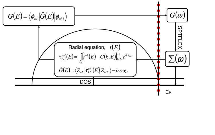
Figure 1: The complex energy contours used within the selfconsistent LDA+DMFT approach, combined with the KKR formalism. The solution of the radial equation allows the evalaution of the single site scattering matrix $t(E)$ and the scattering path operator $\tau^{nn^{\prime}}_{L,L^{\prime}}(E)$ from which the KKR Green function is constructed. The projection of the Green function is perfomed according to Eq. (II.1.2). The impurity Green function is then used to solve the many-body problem within the spin polarized $T$-matrix FLEX solver of the DMFT approach.

Finally a description of the flow diagram of the self-consistent LDA+DMFT approach is presented in Fig. (1). The radial equation Eq. 11 provides the set of regular $(Z)$ and $(J)$ irregular solutions of the single-site problem. Together with the $t$ matrix, the scattering path operator $\tau$ Eq.(21) and the KKR Green’s function is constructed Eq. 18. To solve the many-body problem the a projected impurity Green’s function is constructed according to Eq. II.1.2. The LDA Green’s function $G^{nn}_{LL^{\prime}}(E)$ is calculated on the complex contour which encloses the valence band one-electron energy poles. The Padé analytical continuation is used to map the complex local Green’s function $G^{nn}_{LL^{\prime}}(E)$ on the Matsubara axis which is used when dealing with the many-body problem. In the current implementation the perturbative SPTF (spin-polarized $T$-matrix + FLEX) solver of the DMFT problem described above is used. In fact any DMFT solver could be included which supplies the self-energy $\Sigma(\omega)$ as a solution of the many-body problem. The Padé analytical continuation is used once more to map back the self-energy from the Matsubara axis to the complex plane, where the new local Green’s function is calculated. As was described in the previous sections, the key role is played by the scattering path operator $\tau^{nn}_{L,L^{\prime}}(E)$, which allows us to calculate the charge at each SCF iteration and the new potentials that are used to generate the new LDA Green’s function. In practice it turns out that the self-energy converges faster than the charge density. Of course double counting corrections have to be considered explicitly when calculating the total energy (not done here). Concerning the self-energy used here the double counting corrections are included when solving the many-body problem (see Ref. KL02, ).

III Results and Discussion

To demonstrate the capability of our approach we first applied it to the $3d$ metals Ni and Fe. Although these metals are more or less adequately described in the framework of standard LDA, nevertheless, there are some features in the experimental properties which are due to correlation effects that are not adequately described on this basis. In addition, there are numerous investigations in the literature that seek for an improved description of correlation effects in these systems and that can be compared with.

III.1 Numerical details

The self-consistent LDA+DMFT calculations were carried out for the experimental ground state crystal structures, i.e. fcc for Ni, bcc for Fe and fcc for Ni rich Fe_xNi_1-x alloys. The lattice parameters were fixed at the experimental values (Fe: 5.406 a.u., Ni: 6.658 a.u., for Fe_xNi_1-x: see Ref.Was90, ). The Green’s function was calculated for 32 energy points distributed over semicircular contour. The Brillouin zone integration has been performed on a uniform grid, taking into account the symmetry of the system. As a suitable reference wave functions $\phi_{L}(\vec{r}-\vec{R})$ we have choosen a radial solution of the Schrödinger equation for the spherically symmetric LDA non-magnetic potential, that is determined for an appropriate energy (E=0.7 Ry). The DMFT parameters, average Coulomb interaction $U$, exchange energy $J$, and temperature $T$ used in the calculations are listed in Table 1.

III.2 Results for bcc-Fe and fcc-Ni

To demonstrate the applicability of the scheme presented above band-structure calculations for bcc-Fe and fcc-Ni have been performed. The results of LDA+DMFT calculation for both systems have been already several times discussed in detail in the literature DJK99 ; LKK01 ; CVA+03 .

The density of states curves resulting from a plain LDA and a LDA+DMFT calculations are shown in Figs. 2 and 3 for Fe and Ni, respectively. For the LDA+DMFT calculations we used the DMFT parameters as given in Table 1. The density of states curves for Fe and Ni are in reasonable agreement with corresponding previous LMTO+DMFT DJK99 , as well as EMTO+DMFT CVA+03 calculations. The same is true also for the spin magnetic moments (see Table 1). The spin magnetic moments are some what higher in comparison with the EMTO+DMFT results.CVA+03 From Figs.2 and 3 one can see that in bcc-Fe the correlation effects are much less pronounced than in fcc-Ni. This is due to the large exchange splitting for Fe and the bcc-structure dip in the minority density of states LKK01 . In the case of Ni the LDA+DMFT calculations account for all expected influences of the density of states in satisfying way. As can be seen from Fig. 3, the density of states reflects all three main correlation effects: the $30\%$ narrowing of the occupied part of the d-band, about $40\%$ decrease of exchange splitting and the presence of the famous 6eV satellite compared to the LDA DOS. However, the position of the 6eV sattelite is shifted somewhat to lower binding energies. This shift and the large broadening of the resonance is due to the perturbation approach of the DMFT solver of the effective impurity problem used here.KL02

III.3 Results for fcc-Fe_xNi_1-x disordered alloy

As mentioned above, the scheme presented here allows in a straight forward way to deal with disordered alloys. To demonstrate how this works we carried out a set of LDA as well as LDA+DMFT calculations for fcc-Fe_xNi_1-x disordered alloy for various concentrations. For the LDA+DMFT we used the same DMFT parameters (U, J and T) as in the case of pure bcc-Fe and fcc-Ni (see Table 1). In Fig. 4 the element resolved as well as the total spin magnetic moments are shown. Although the difference between LDA and LDA+DMFT moments for Fe is rather small one can see an interesting trend. In contrast to the pure bcc-Fe case the LDA+DMFT moments for Fe in fcc-Fe_xNi_1-x alloy are slightly larger than corresponding LDA ones. In the case of Ni, on the other hand, a decrease of the magnetic moment was obtained as in the case of pure fcc-Ni (see Table 1). Comparing the average moments in Fig. 4 with experiment Was90 one finds rather good agreement already for LDA-based spin moment. In spite of its present limitations, the LDA+DMFT scheme does not spoil the overall behaviour for the concentration dependence of magnetic moments.

Finally, in Fig. 5 the resulting concentration dependence of the self-energy is shown. We present the results for the real part of the self-energies for Fe and Ni atoms for the $t_{2g}$ symmetry (the results for the $e_{g}$ symmetry are similar and hence not plotted). It is interesting to note that the slope of the self-energy near Fermi level $Z=\frac{d\Sigma}{dE}|_{E=E_{F}}$ which defines the mass renormalisation and leads to the narrowing of the band practically does not depend on the concentration. On the other hand, for the high energy part of the self-energy one sees rather noticeable differences giving raise to the changes in the sattelite structure.

IV Summary

A scheme has been presented that allows to combine the KKR band structure method and the LDA+DMFT approach to deal with correlated systems. Its applicability has been demonstrated by results for ferromagnetic bcc-Fe and fcc-Ni. For this systems a good agreement with previous LDA+DMFT methods has been found. In addition we combined LDA+DMFT scheme with the CPA to deal with disordered alloy. As an example we presented results for fcc-Fe_xNi_1-x disordered alloy.

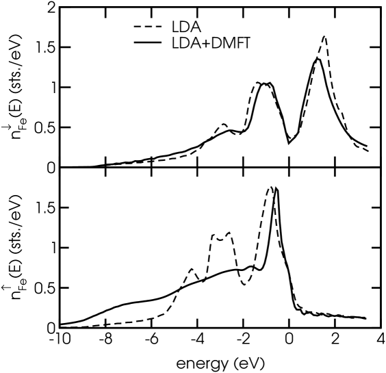
Figure 2: Spin resolved density of states of bcc-Fe as calculated within LDA(dashed line) and LDA+DMFT (full line) using the KKR-method. (DMFT parameters: U=2eV, J=0.9eV, T=400K)

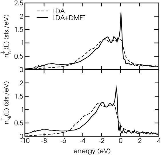
Figure 3: Spin resolved density of states of fcc-Ni as calculated in the LDA (dashed line) and LDA+DMFT (full line) using the KKR-method. (DMFT parameters: U=3eV, J=0.9eV T=400K)

Figure 4: Spin magnetic moments of Fe (circles) and Ni (squares) in Fe_xNi_1-x alloy calculated using plain LDA (open symbols) and the LDA+DMFT method (full symbols).

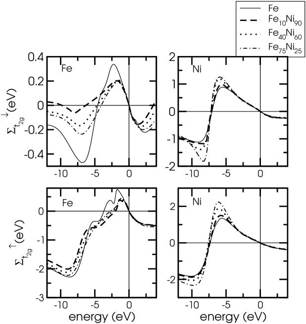
Figure 5: Left: Concentration dependence of the real part of the spin resolved self-energy for Fe. Only results for $t_{2g}$ d-orbitals are shown. Right: Same as in the left panel but for Ni

Table 1: The DMFT parameters average Coulomb interaction U, exchange energy J and temperature T used in the calculations for bcc-Fe, fcc-Ni and fcc-Fe₅₀Ni₅₀. In addition the theoretical spin magnetic moments as calculated by the LDA and the LDA+DMFT methods are shown for bcc-Fe and fcc-Ni. Magnetic moments for fcc-Fe_xNi_1-x alloy are presented in Fig. 4

	U(eV)	J(eV)	T(K)	$\mu_{spin}^{LDA}(\mu_{B))}$	$\mu_{spin}^{DMFT}(\mu_{B))}$
bcc-Fe	2.0	0.9	400	2.29	2.28
fcc-Ni	3.0	0.9	400	0.59	0.57
Fe in FexNi1-x	2.0	0.9	400
Ni in FexNi1-x	3.0	0.9	400

References

- (1) J. Korringa, Physica XIII, 392 (1947).
- (2) W. Kohn and N. Rostoker, Phys. Rev. 94, 1111 (1954).
- (3) J. S. Faulkner, Prog. Mater. Sci. 27, 3 (1982).
- (4) A. Georges, G. Kotliar, W. Krauth, and M. J. Rozenberg, Rev. Mod. Phys. 68, 13 (1996).
- (5) V. Drchal, V. Janis, and J. Kudrnovsky, Phys. Rev. B 60, 15664 (1999).
- (6) I. Turek et al., Electronic structure of disordered alloys, surfaces and interfaces (Kluwer Academic Publ., Boston, 1997).
- (7) J. Hubbard, Proc. Roy. Soc. (London) A 281, 401 (1964).
- (8) J. R. Taylor, Scattering Theory: The Quantum Theory of Non-relativistic Collision (Krieger Publ. Comp., Malabar, FL, 1987).
- (9) O. K. Andersen, O. Jepsen, and G. Krieger, in Lectures on methods of electronic structure calculations, edited by V. Kumar, O. K. Andersen, and A. Mookerjee (World Scientific Publ. Comp., Singapore, 1994), p. 63.
- (10) O. K. Andersen and T. Saha-Dasgupta, Phys. Rev. B 62, R16219 (2000).
- (11) L. Vitos, H. L. Skriver, B. Johansson, and J. Kollar, Comp. Mater. Science 18, 24 (2000).
- (12) L. Chioncel, L. Vitos, I. A. Abrikosov, J. Kollar, M. I. Katsnelson, and A. I. Lichtenstein, Phys. Rev. B 67, 235106 (2003).
- (13) L. Vitos, Phys. Rev. B 64, 014107 (2001).
- (14) V. I. Anisimov et al., Journal of Physics: Condensed Matter 9, 7359 (1997).
- (15) A. I. Lichtenstein and M. I. Katsnelson, Phys. Rev. B 57, 6884 (1998).
- (16) M. Katsnelson and A. Lichtenstein, Journal of Physics: Condensed Matter 11, 1037 (1999).
- (17) S. Y. Savrasov, G. Kotliar, and E. Abrahams, Nature 410, 793 (2001).
- (18) S. Y. Savrasov and G. Kotliar, Phys. Rev. B 69, 245101 (2004).
- (19) A. I. Lichtenstein, M. I. Katsnelson, and G. Kotliar, in Electron Correlations and Materials Properties II, edited by A. Gonis, N. Kioussis, and M. Ciftan (Kluwer/Plenum, Berlin, 2002), p. 428.
- (20) K. Held et al., in Quantum Simulations of Complex Many-Body Systems: From Theory to Algorithms, NIC Series, edited by J. Grotendorst, D. Marx, and A. Muramatsu (NIC, Juelich, 2002), Vol. 10, p. 175.
- (21) L. Chioncel, M. I. Katsnelson, R. A. de Groot, and A. I. Lichtenstein, Phys. Rev. B 68, 144425 (2003).
- (22) B. L. Gyorffy, Phys. Rev. B 5, 2382 (1972).
- (23) G. Rickayzen, in Green’s functions and condensed matter, edited by N. H. March (Academic Press, London, 1984).
- (24) J. S. Faulkner and G. M. Stocks, Phys. Rev. B 21, 3222 (1980).
- (25) P. Weinberger, Electron Scattering Theory for Ordered and Disordered Matter (Oxford University Press, Oxford, 1990).
- (26) V. I. Anisimov, J. Zaanen, and O. K. Andersen, Phys. Rev. B 44, 943 (1991).
- (27) V. Anisimov, F. Aryasetiawan, and A. Lichtenstein, J. Phys.: Condensed Matter 9, 767 (1997).
- (28) N. E. Bickers and D. J. Scalapino, Ann. Physik 193, 206 (1991).
- (29) H. Ebert and B. L. Gyorffy, J. Phys. F: Met. Phys. 18, 451 (1988).
- (30) R. Zeller, J. Phys. C: Solid State Phys. 20, 2347 (1987).
- (31) E. Tamura, Phys. Rev. B 45, 3271 (1992).
- (32) V. M. Galitski, Zh. Exper. Theor. Fiz. 34, 115, 1011 (1958).
- (33) J. Kanamori, Progr. Theor. Phys. 30, 275 (1963).
- (34) M. I. Katsnelson and A. I. Lichtenstein, European Physical Journal B 30, 9 (2002).
- (35) P. A. Lee and T. V. Ramakrishnan, Rev. Mod. Phys. 30, 9 (1985).
- (36) B. Belitz and T. R. Kirkpatrick, Rev. Mod. Phys. 1994, 261 (66).
- (37) V. Dobrosavljevic and G. Kotliar, Phys. Rev. B 50, 1430 (1994).
- (38) P. Soven, Phys. Rev. 156, 809 (1967).
- (39) H. Ebert and H. Akai, Mat. Res. Soc. Symp. Proc. 253, 329 (1992).
- (40) E. F. Wassermann, in Ferromagnetic Alloys, edited by K. H. J. Buschow and E. P. Wohlfarth (North-Holland, Amsterdam, 1990), Vol. 5, p. 238.
- (41) A. I. Lichtenstein, M. I. Katsnelson and G. Kotliar, Phys. Rev. Letters 87, 067205 (2001).