The Multimode Conductance Formula
for a Closed Ring

Abstract

The multimode conductance of a closed ring is found within the framework of a scattering approach. The expression can be regarded as a generalization of the Landauer formula. The treatment is essentially classical because we assume short coherence time. Our starting point is the Kubo formalism, but we also use a master equation approach for the derivation. As an example we calculate the conductance of a multimode waveguide with an attached cavity.

1 Introduction

The notion of conductance has gone several transformation in the last century. In the mesoscopic community [1, 2], following Landauer, it is customary nowadays to consider the open geometry that is described in Fig.1a, where a device is attached to left and right reservoirs, and the bias is understood as emerging from a chemical potential difference. For a single mode device it is argued that the conductance is essentially the transmission, while for a multimode device with “spinless” electrons

$$G_{\mbox{\tiny Landauer}}=\frac{e^{2}}{2\pi\hbar}\sum_{n,m}g^{T}_{nm}$$ (1)

where $g^{T}_{nm}$ is the transmission matrix. We can optionally assume that the chemical potential of the two reservoirs is the same, and consider the effect of an electro motive force (EMF) such that the voltage drop is concentrated across a segment of the device. More generally we can consider the problem of driving a current by changing the electrical potential at some region of the device. The latter more general problem is known as “quantum pumping”. The calculation of the “geometric” conductance in the latter case leads to the Büttiker-Prétre-Thomas (BPT) formula [3], which is a generalization of the Landauer formula Eq.(1).

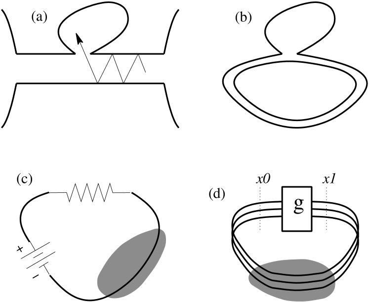
Figure 1: Panel (a) displays the standard Landauer (open) geometry of connecting a conductor to a left and a right reservoirs. In this illustration the conductor is a rectangular waveguide to which a cavity is attached. In panel (b) the leads are joined together so as to form a ring. The motion in the ring is assumed to be chaotic due to the scattering in and out of the cavity. Panel (c) is the schematic electrical engineering representation of the system. In panel (d) the system is modeled as a network. The scattering region is described by the transition matrix $g_{ab}$. In (c) and in (d) we indicate the presence of the environment by the gray shading. In fact (a) can be regarded as a special case of (b) provided one assumes that the effect of the environment is to randomize the velocity within the wire region. The current is measured via the section $x=x_{1}$. The Electro motive force (EMF) is realized by time dependent Aharonov Bohm flux. The voltage drop can be concentrated anywhere along the ring (say across $x=x_{0}$). Setting a chemical potential difference in the setup of panel (a) can be regarded as such particular option.

It is quite natural to ask what happens if the two leads are detached from the reservoirs, and the system is closed into a ring as in Fig.1b [4, 5]. Still we can induce EMF by changing in time an Aharonov-Bohm magnetic flux, or we can change the potential in some region of the device, so as to get an electrical current. In spite of much interest in closed mesoscopic rings a straightforward answer to this simple question has not been given. We shall review later the main published statements [6, 7, 8, 9, 10, 11]

In this paper we are interested in circumstances such that the leading result for the conductance is of classical nature. This is completely analogous to the discussion of diffusive rings in circumstances such that the leading result is given by the Drude formula. We are going to assume that the coherence time is shorter than the time that it takes for an electron to encircle the ring. Thus, as far as the dynamics is concerned, our analysis is essentially of classical nature. The case of a fully coherent ring requires further analysis which is beyond the scope of the present work. Therefore it will be discussed in separate publications: The one-mode case in [14] and the multi-mode case in [15].

It is important to realize that our assumption of short coherence time is plays analogous role to that which is played by the reservoirs in the Landauer-BPT formalism. In fact we are going to explain that the Landauer-BPT formalism can be regarded as a special limit of the problem that we are going to consider. This will further illuminate the formal discussion in [4].

1.1 Motivation

The interest in the response of small mesoscopic rings is long standing [6, 7, 8, 9, 10]. Measurements of the the conductance of closed mesoscopic rings has been performed already 10 years ago [11]. In a practical experiment a large array of two dimensional rings is fabricated. The conductance measurement can be achieved via coupling to a highly sensitive electromagnetic superconducting micro-resonator. In such setup the EMF is realized by creating a current through a ”wire” that spirals on top of the array, and the conductance of the rings is determined via their influence on the electrical circuit. Another possibility is to extract the conductance from the rate of Joule heating. The later can be deduced from a temperature difference measurement assuming that the thermal conductance is known.

We do not think that there is any problem to design rings of the type which is illustrated in Fig. 1. The question is why to bother? This brings us to the theoretical motivation for this work. Past theoretical studies are quite well summarized by the paper “(Almost) everything you always wanted to know about the conductance of mesoscopic systems” [10] and see references therein. The major interest was in diffusive rings, and the main issue was weak localization corrections to the Drude result taking into account the level statistics, the type of occupation, etc. Our interest is in a different type of configuration, which is motivated by “quantum chaos” studies. Our claim (see next subsection) that the conductance of a closed ring can be larger than the number of open modes is quite unorthodox.

More importantly: Our approach to the problem of mesoscopic conductance has a practical appeal. The reason for the popularity of the scattering approach in mesoscopic physics is its ”plug and play” feature. The experimentalist is able to characterize the scattering properties of his/her device, and then he/she is able to make a prediction regarding the conductance. It is only natural to extend this ”plug and play” approach to the analysis of conductance of closed rings. This extension is far from being trivial, as we explain later (in section 6).

We care to make clear distinction between classical and quantal effects. This helps to develop a better intuition for the physics of such devices. The approach in the present work is in the spirit of the Boltzmann picture: The scattering “cross section”, which is possibly of quantum mechanical nature, is taken as an input, while the overall dynamics is assumed to be of classical nature. The implications of quantum interference will be discussed in future works [14, 15].

1.2 specific results

The conductance of a single mode ring ($\mathcal{M}=1$) with a stochastic scatterer that has transmission $g_{T}$ is given by the expression

$$G=\frac{e^{2}}{2\pi\hbar}\left[\frac{g_{T}}{1-g_{T}}\right]$$ (2)

We shall show that the multimode generalization of this formula is:

$$G=\frac{e^{2}}{2\pi\hbar}\sum_{nm}\left[2g^{T}/(1-g^{T}+g^{R})\right]_{nm}$$ (3)

where $g^{T}_{nm}$ and $g^{R}_{nm}$ are the $\mathcal{M}\times\mathcal{M}$ transmission and reflection blocks of the transition matrix, As an example we analyze the system of Fig.1a. We find that the Landauer formula gives

$$G_{\mbox{\tiny Landauer}}\approx\frac{e^{2}}{2\pi\hbar}\left[1-\frac{1}{4}\alpha\right]\mathcal{M}$$ (4)

where $\alpha$ is the dimensionless size of the opening to the cavity. In contrast to that for the multi-mode conductance of the corresponding ring structure (Fig.1b) we get

$$G\approx\frac{e^{2}}{2\pi\hbar}\left[\frac{1}{\alpha}(1+\ln(2\mathcal{M}))\right]\mathcal{M}$$ (5)

Unlike the case of the Landauer conductance, the result does not reflect the number of open modes. This is because the contribution of the low modes is singular in the limit of small $\alpha$. Furthermore, the conductivity (conductance per channel) diverges logarithmically in the classical limit.

1.3 Outline

We define the model system in sections 2 and 3 and the notion of conductance in section 4. In section 5 we argue that the notion of conductance is meaningful even in the absence of a bath. We further discuss the role of the environment in section 6, where we make distinguish between various type of bath induced effects.

As explained in section 7 the purpose of the “linear response analysis” is to find the stationary-like state of the driven system. The procedure is to assume that in the absence of driving the system would be in a (strict) stationary state, which we regard as the zero order solution. Then we try to find a first order solution (in the EMF) to the time dependent problem.

In sections 8 and 9 we discuss the Kubo approach to linear response. We take the simplest route following Refs.[12, 16, 17, 18] leading to the fluctuation-dissipation version of the Kubo formula. The application of the Kubo formula to the analysis of the single mode conductance is presented in sections 10 and 11. The relation to the Landauer result is clarified in section 12.

There are many (equivalent) ways to do “linear response analysis”. It turns out that the derivation of the multi-mode conductance formula becomes more transparent by adopting a master equation approach. This is carried out in section 13.

Throughout the paper, and in particular in the concluding section, we emphasize that our approach has a straightforward extension to the analysis of quantum pumping. The Kubo approach allows a better understanding of the role which is played by the environment, and makes it possible to bridge between the strict quantum adiabatic limit and the other extreme limit of having an open geometry.

2 Setting up the model

Consider non-interacting spinless electrons in a ring, as in Fig.1b. The one-particle Hamiltonian is

$${\cal H}=\frac{1}{\mathsf{m}}(\bm{p}-e\Phi a(\bm{r}))^{2}+V(\bm{r})$$ (6)

where $\mathsf{m}$ and $e$ are the mass and the charge respectively. The vector potential which is associated with the flux $\Phi$ is described by

$$\oint a(\bm{r})\cdot d\bm{r}=1$$ (7)

The dimensionality of the ring is $d$. The ring consists of a “wire” region and a scattering region. The motion of the particle inside the ring is assumed to be globally chaotic. The coordinate along the wire will be denoted as $x$. The scattering region is located at $x\sim 0$.

In the geometry of Fig.1b the “wire” is a $d=2$ waveguide of width $L_{\perp}$. Later we describe the waveguide as a set of $d=1$ wires (Fig.1d) such that each “wire” corresponds to an open mode of the waveguide. The length of the ring $L$ is assumed to be large compared with the scattering region so as to allow meaningful definition of a scattering matrix in the quantum mechanical analysis (evanescent modes are ignored).

The ring is driven by a time dependent Aharonov-Bohm flux. The EMF $-\dot{\Phi}$ is assumed to be constant. There are various ways to introduce the EMF into the ring. One possibility is to have all the voltage drop over a section at $x=x_{0}$. Namely,

$$a(x)=\delta(x-x_{0})$$ (8)

For sake of later analysis we define a generalized force which is associated with the flux:

$${\cal F}=-\frac{\partial{\cal H}}{\partial\Phi}=e\hat{v}\delta(\hat{x}-x_{0})$$ (9)

where $v$ is the velocity in the $x$ direction. In the quantum mechanical case a symmetrization is implicit. This is in fact a current operator. Obviously we do not have to measure the current at the same point where we apply the voltage. So for sake of generality we introduce the notation

$$\mathcal{I}=e\hat{v}\delta(\hat{x}-x_{1})$$ (10)

We also note that with uniform averaging over $x_{1}$ we get $(e/L)\hat{v}$ which is essentially the velocity operator.

In the absence of driving the “pure” stationary states of the system are the microcanonical states. We use classical language but also have in mind a semiclassical picture. Each microcanonical state occupy a shell whose phase space volume is $(2\pi\hbar)^{d}$. The density of states is

$$\mathsf{g}(E)=\int\int\frac{d\mathbf{r}d\mathbf{p}}{(2\pi\hbar)^{d}}\delta(E-\mathcal{H}(\mathbf{r},\mathbf{p}))$$ (11)

The zero order stationary state is characterized by an occupation function $f(E)$. Later we shall take it to be the Fermi function. Thus

$$dN=\rho(\mathbf{r},\mathbf{p})\frac{d\mathbf{r}d\mathbf{p}}{(2\pi\hbar)^{d}}=f(E)\frac{d\mathbf{r}d\mathbf{p}}{(2\pi\hbar)^{d}}$$ (12)

where $E=H(\bm{r},\bm{p})$ is the energy. The distribution of the particles in energy is

$$\rho(E)=\mathsf{g}(E)f(E)$$ (13)

and the total number of particles is

$$N=\int\int\rho(\mathbf{r},\mathbf{p})\frac{d\mathbf{r}d\mathbf{p}}{(2\pi\hbar)^{d}}=\int_{-\infty}^{\infty}\rho(E)dE=\int_{-\infty}^{\infty}f(E)\mathsf{g}(E)dE$$ (14)

3 Network modeling

A network is defined as a set of 1D wires that are connected in vertices. The network Hamiltonian is ill defined in the classical limit because the the scattering in each vertex is described by a scattering matrix. In particular for the model of Fig.1d the scattering is described by a scattering matrix $S_{ab}$, and we define the corresponding transition matrix as $g_{ab}=|S_{ab}|^{2}$. Thus the classical description of the system is stochastic rather than deterministic.

Still we can regard networks as an effective way to describe the chaotic dynamics [19]. The reason is that upon coarse graining a chaotic system looks like a stochastic model. Specifically, in the case of the system of Fig1b, quantum mechanics introduces “coarse graining” in a most natural way. Each mode in the scattering problem can be regarded as a 1D wire with the dispersion relation

$$v_{n}=\frac{1}{\mathsf{m}}\sqrt{2\mathsf{m}E-\left(\frac{\pi\hbar}{L_{\perp}}n\right)^{2}}$$ (15)

where $E$ is the energy of the particle, and $L_{\perp}$ is the width of the waveguide. The open modes are are those for which $v_{n}$ is a real number. We shall denote the number of open modes by $\mathcal{M}$ hence the number of open channels in the open geometry is $2\mathcal{M}$.

The density of states of the system can be written as a sum over single-mode expressions:

$$\mathsf{g}(E)=\mathsf{g}_{\mbox{\tiny dot}}(E)+2\sum_{n=1}^{\mathcal{M}}\frac{L}{(2\pi\hbar)}\frac{1}{v_{n}(E)}$$ (16)

where the factor of two takes into account both clockwise and anticlockwise motion. A stationary state of the system is described by the distribution functions $\rho_{n}^{\rightarrow}(E)$ of the clockwise moving particles and $\rho_{n}^{\leftarrow}(E)$ of the counter-clockwise moving particles. The index $n$ distinguishes different modes. The normalization is such that

$$N=\int\rho_{\mbox{\tiny dot}}(E)dE+L\sum_{n}\int(\rho_{n}^{\rightarrow}(E)+\rho_{n}^{\leftarrow}(E))dE$$ (17)

The density of particles per unit length in a given mode is implied by Eq.(13):

$$\rho_{n}^{\rightarrow}(E)dE=\rho_{n}^{\leftarrow}(E)dE=\frac{dE}{(2\pi\hbar)v_{n}(E)}f(E)$$ (18)

Note that for a microcanonical distribution $dE$ can be regarded as a fixed parameter that defines an energy window or a width of an energy shell.

The scattering is described by a $2\mathcal{M}\times 2\mathcal{M}$ transition matrix that has a block structure:

$$g_{ab}=\left(\matrix{g^{R}&g^{T}\cr g^{T}&g^{R}}\right)$$ (19)

It consists of the reflection matrix $g^{R}_{nm}$ and the transmission matrix $g^{T}_{nm}$. Note that the channel index $a$ contains both mode specification and left/right lead specification. We assume time reversal invariance, so as to have a symmetric matrix. For clarification we note that if $N$ particles incident in channel $b$, then $g_{ab}N$ particles emerge in channel $a$. This means that $g_{ab}$ is the ratio between ingoing and outgoing fluxes. In the ergodic state Eq.(18) implies that $\rho_{a}\propto 1/v_{a}$. Therefore we have detailed balance:

$$g_{ab}\,\rho_{b}v_{b}\,\,=\,\,g_{ba}\,\rho_{a}v_{a}\ \ \ \ \ \ \ \mbox{[no summation]}$$ (20)

Namely, for a stationary state the transitions from $a$ to $b$ are exactly balanced by the transitions from $b$ to $a$.

4 Definition of the conductance

If the EMF is not too large we expect to have Ohmic behavior ${\langle\mathcal{I}\rangle\propto\mbox{EMF}}$. Hence we define the conductance via the relation

$$\langle\mathcal{I}\rangle=-G\dot{\Phi}$$ (21)

This is in fact a special case of a more general concept of conductance. In the theory of “quantum pumping” we may vary in time some other parameter $X$, and get current $\langle\mathcal{I}\rangle\propto\dot{X}$. Hence we can define (generalized) conductance via

$$\langle\mathcal{I}\rangle=-G\dot{X}$$ (22)

Much of the formalism that we are going to use can be extended to handle this more general case. However, in what follows we restrict ourselves to the case of an EMF driven system.

Still one can wonder whether it is important to specify how the EMF is introduced. Does it matter how $a(x)$ look like? The answer is that within linear response theory all the choices lead to the same result. This is not merely a gauge issue because for different $a(x)$ the electric field along the ring does not look the same. Namely, if the gauge of the vector potential is changed

$$a(x):=a(x)+(d/dx)v(x)$$ (23)

then the new scalar potential is

$$V(x):=V(x)-e\dot{\Phi}v(x)$$ (24)

Thus a different choice for $x_{0}$ can be regarded as associated with adding a rectangular barrier of height $e\dot{\Phi}$. Within linear response it is assumed that $e\dot{\Phi}$ is too small to make any difference. If this assumption is not applicable, it is no longer the “linear response regime”, and the specification of $a(x)$ becomes significant.

5 The long time scenario

Some people find it inappropriate to define conductance for a closed system because the problem does not possess a stationary solution [22]. Namely, it is clear that without a contact to a thermal bath the driven system is gradually heated up. However, we find this objection of no relevance. The practical point of view of an electrical engineer is demonstrated in Fig.1c. It is clear that at any moment the engineer is inclined to characterize the ring by its conductance. This is true irrespective of whether there is a contact with a thermal bath or not. In the absence of such contact it is evident that the system is heated up and therefore the conductance becomes time-dependent.

It is true that the overall scenario is (formally) beyond linear response, but it is also true that at a given instant of time it is feasible to have a valid linear response description. The validity condition is having an ergodization time which is much smaller than the time that it takes to have a significant change in the (evolving) energy distribution of the system. This reasoning leads to “slowness conditions” that are further discussed in Ref.[17].

We note that there is a strict analogy here with the strategy of analyzing quantum pumping. Also there the conductance $G(X)$ is calculated, using either BPT or the Kubo formula, for various points $X=(X_{1},X_{2})$ in parameter space. Later the pumped charge is expressed as a line integral over the conductance:

$$Q=\oint\langle\mathcal{I}\rangle dt=\oint[-G(X(t))\cdot\dot{X}]dt=-\oint G\cdot\vec{dX}$$ (25)

Consequently the pumped charge is not proportional to the amplitude of the driving cycle. Thus we can get (globally) “non linear response” out of (momentary) linear response analysis. See [5] for more details.

6 Digression: The role of the environment

On the mathematical side we have already defined precisely the assumptions in the basis of the derivation that we are going to present. The purpose of the present section is to further clarify the physical circumstances that justify these assumptions. Also we would like to put the present work in context of past literature. This section can be skipped in first reading.

6.1 Quantum to classical correspondence

Our first step is to define a feasibility condition for the validity of a semiclassical treatment. Assuming that the total transmission of the device is $g_{T}\sim 1$ the time for the randomization of the velocity is

$$\tau_{cl}\ \approx\ \left(\frac{1}{1-g_{T}}\right)\times\frac{L}{v_{F}}$$ (26)

where $L$ is the length of the ring, and $v_{F}$ is the Fermi velocity. On the other hand the time that it takes to resolve the quantized energy levels of the ring is

$$t_{\mbox{\tiny Heisenberg}}\ \approx\ \mathcal{M}\times\frac{L}{v_{F}}$$ (27)

Hence the quantum-to-classical correspondence condition is

$$\mathcal{M}\ \gg\ \frac{1}{1-g_{T}}$$ (28)

which is always satisfied in the classical limit. Note that the limit $\mathcal{M}\rightarrow\infty$ is analogous to $\hbar\rightarrow 0$.

6.2 Single mode rings

In the case of a single mode ring (a one dimensional ring with a delta scatterer) a classical treatment of the dynamics does not make any sense in view of the correspondence condition of the previous subsection. The analysis should be purely quantum mechanical and issues such as Landau-Zener transitions [12], Debye relaxation mechanism [7] and Dynamical Localization [9, 13] should be taken into account. Recently we have introduced a new ingredient into the analysis that sheds a new light on the whole issue [14].

6.3 Multi mode diffusive rings

In the case of multi mode diffusive ring the leading order result for the conductance is as expected just the classical Drude expression. The typical calculation [8] assumes that the levels are “broadened” due to the interaction with the environment. In the major case of interest the level broadening $\Gamma$ is assumed to be larger than the mean level spacing $\Delta$ but much smaller than any semiclassical energy scale. Hence it barely affects the Drude result. Still it determines the quantum weak localization correction, which turns out to be of order $\Delta/\Gamma$. The weak localization correction depends on the levels statistics and therefore on the magnetic flux. Hence it can be detected in an actual experiment [11].

6.4 Multi mode ballistic rings

In the present work we consider a multi mode ballistic ring rather than a diffusive ring. This means that the time to randomize the velocity can be much larger than the time $L/v_{F}$ to make one round along the ring. This implies that in our configuration the conductance (in natural units) can be larger than the number of open modes.

We assume that the environment induces level broadening $\Gamma$ which is larger than $\hbar v_{F}/L$. Hence we derive the leading (classical) term and do not take into account the implications of quantum interference. To put this assumption in a larger perspective we make the following classification:

• Isolated system (no environment).

• The bath induces only decoherence effect.

• The bath induces velocity randomization.

• Bath limited dynamics.

The first case of fully coherent dynamics will be analyzed in [15]. We consider in this work only the second case. Still we would like to further explain why the second case is physically typical, and to make some comments on the other two cases.

6.5 The decoherence mechanism

It is typical to assume that the fluctuations of the environment are of large spatial correlation length compared with $L_{\perp}$. An extreme case is the Caldeira-Leggett modeling which assumes an infinite correlation length. The matrix elements of the position variable scale like $L_{\perp}$ for inter-mode transitions and like $L$ for intra-mode transitions. Hence inter-mode transitions are rare compared with intra-mode transitions, the ratio being $(L_{\perp}/L)^{2}$. Therefore it is realistic to consider circumstances such that velocity randomization due to the environmental “noise” can be neglected, while intra-mode transitions cannot be neglected. The latter lead to decoherence. The simplest estimate for the decoherence rate is $\Gamma=\eta k_{B}TL^{2}/\hbar$, where $\eta$ characterizes the coupling to the environmental modes, and $T$ is the temperature. Thus we see that case 2 is physically typical.

6.6 Velocity randomization

If the fluctuations are strong enough inter-mode transitions cannot be ignored. This would lead to randomization of the velocity in the wire region. The scenario of having a bath that just randomizes the velocity, but does not affect the transmission of the ring is apparently not of much physical interest. Still such effect can be realized artificially, and it is of pedagogical importance, as discussed in section 12.

6.7 Bath limited dynamics

If the interaction with the environment determines the transmission of the ring, we get to case 4. The most obvious example is the the analysis of conductance in room temperatures. The scattering and hence the diffusion of the particles is dominated by bath induced inelastic scattering by phonons.

The main point regarding case 4 is that the bath cannot be eliminated from the model analysis. Another example for such circumstances is provided by the Debye dissipation mechanism [7]. The latter assumes that the inelastic relaxation time is much shorter compared with the adiabatic variation of the energy levels, leading to time lag between the driving cycle and the adjustment of the occupation probabilities.

7 Linear response analysis

The simplest route to linear response theory [12, 16, 17, 18] takes the relation $d\mathcal{H}/dt=\partial\mathcal{H}/\partial t$ as a starting point. It follows that the change in the energy of a particle is given with no approximation by the formula

$$\mathcal{H}(t)-\mathcal{H}(0)=-\dot{\Phi}\int_{0}^{t}\mathcal{F}(t^{\prime})dt^{\prime}$$ (29)

By squaring and averaging over initial conditions we get that the second moment as a double time integral over $\langle\mathcal{F}(t^{\prime})\mathcal{F}(t^{\prime\prime})\rangle$. Within linear response this correlation is approximated by the stationary correlation function

$$C(t^{\prime}-t^{\prime\prime})=\langle{\cal F}(t^{\prime}){\cal F}(t^{\prime\prime})\rangle_{E}$$ (30)

where the average on the right hand side is taken with a zero order microcanonical solution. Thus one concludes that there is a diffusion in energy, with the coefficient

$$D_{E}=\dot{\Phi}^{2}\times\frac{1}{2}\int_{-\infty}^{\infty}C(\tau)d\tau$$ (31)

Next one wants to see what happens in the more general case of an arbitrary $f(E)$. On long times it is argued that the probability distribution $\rho(E)$ satisfies the following diffusion equation:

$$\frac{\partial\rho}{\partial t}\ =\ \frac{\partial}{\partial E}\left(\mathsf{g}(E)D_{E}\frac{\partial}{\partial E}\left(\frac{1}{\mathsf{g}(E)}\rho\right)\right)$$ (32)

The energy of the system is $\langle{\cal H}\rangle=\int E\rho(E)dE$. It follows that the rate of energy absorption is

$$\frac{d}{dt}\langle{\cal H}\rangle=-\int_{0}^{\infty}dE\ \mathsf{g}(E)\ D_{E}\ \frac{\partial}{\partial E}\left(\frac{\rho(E)}{\mathsf{g}(E)}\right)$$ (33)

For zero temperature Fermi occupation we get

$$\frac{d}{dt}\langle{\cal H}\rangle\ =\ \left[\mathsf{g}(E)\frac{}{}D_{E}\right]_{E=E_{F}}\ =\ G\dot{\Phi}^{2}$$ (34)

This is the mesoscopic version of Joule law. The expression for the conductance is

$$G=\mathsf{g}(E_{F})\times\frac{1}{2}\int_{-\infty}^{\infty}C(\tau)d\tau$$ (35)

8 The Kubo formula

The above is apparently the simplest and most illuminating derivation of the Fluctuation-Dissipation version of the Kubo formula. A more complicated treatment [18, 4, 5] allows to write a generalized version that holds also for “quantum pumping” applications. Namely,

$$G=\mathsf{g}(E_{F})\times\int_{0}^{\infty}C(\tau)d\tau$$ (36)

with

$$C(\tau)=\langle{\cal I}(\tau){\cal F}(0)\rangle_{E}$$ (37)

where $\mathcal{F}$ is the generalized force which is associated with the driving. In the present application $\mathcal{F}$ is just the current operator, hence $C(\tau)$ is symmetric, and therefore the generalized version Eq.(36) is equivalent to Eq.(35).

It is also important to make a connection with the more traditional treatment of conductance in case of disordered metals. If we set $a(x)=1/L$ for the vector potential we get $(e/L)\hat{v}$ as the current operator. Hence we get from Eq.(35)

$$G=\mathsf{g}(E_{F})\times\frac{1}{2}\left(\frac{e}{L}\right)^{2}\int_{-\infty}^{\infty}\langle v(\tau)v(0)\rangle d\tau$$ (38)

The conventional derivation of the Drude formula is based on the assumption of exponential decay of the velocity-velocity correlation function. The latter formula is (formally) valid in any case, but in case of a disordered sample it has special appeal because it implies the Einstein relation between the conductance and the spatial diffusion. Namely, if we have a diffusive ring then it is natural to write $G=\hat{G}/L$ and to define $\hat{\mathsf{g}}(E_{F})=\mathsf{g}(E_{F})/L$. Then we can rewrite Eq.(38) as

$$\hat{G}=e^{2}\hat{\mathsf{g}}(E_{F})D_{\mbox{\tiny space}}$$ (39)

The more conventional derivations of this expression is based on the phenomenological relation $J=-D\nabla(\mbox{density})-\hat{G}\nabla(\mbox{potential})$ and the argument that $J=0$ at equilibrium.

9 Implications of the Kubo formula

From the the Kubo formula Eq.(36) it is not obvious that the result for $G$ is independent of where we measure $\mathcal{I}$. In general it can be proved [20] that for a different choice of $\mathcal{I}$ the corresponding Kubo conductance may differ at most by $e\mathsf{g}(E_{F})\langle\mathcal{F}\rangle$. But if $\mathcal{F}$ is a current operator then $\langle\mathcal{F}\rangle=0$ and therefore the conductance be becomes independent of $x_{1}$.

Also it seems that the Kubo conductance is proportional to the density of states. Therefore, if we had doubled the volume of the cavity, would we get larger conductance? Furthermore, does the result for $G$ depends merely on the transition matrix, and not (say) on the dwell time inside the scattering region?

To answer these questions, and to establish the $x_{1}$ independence of $G$, let us write the Kubo formula in a more illuminating way. By definition we have

$$\int_{-\infty}^{\infty}\langle{\cal I}(\tau){\cal F}(0)\rangle d\tau=\sum_{r}p_{r}{\cal F}_{r}Q_{r}$$

$$\equiv\frac{1}{\mathsf{g}(E)}\int\delta(E-\mathcal{H}(\bm{r},\bm{p}))\frac{d\bm{r}d\bm{p}}{(2\pi)^{d}}F(\bm{r},\bm{p})Q(\bm{r},\bm{p})$$ (40)

where $r$ is an index that labels phase space cells (different initial conditions), and $p_{r}$ corresponds to a microcanonical distribution. We have introduced the notation

$$Q(\bm{r},\bm{p})=\int_{-\infty}^{\infty}{\cal I}(\tau;\bm{r},\bm{p})d\tau$$ (41)

Namely $Q(\bm{r},\bm{p})$ is the total charge which is obtained by integrating the current which is induced by a particle that goes through the point $(\bm{r},\bm{p})$ at $t=0$. It is in fact (for $e=1$) the winding number of the associated trajectory, and therefore it gives a result which is independent of the chosen section. Note however that $Q(\bm{r},\bm{p})$ obtains a meaningful value only upon course graining, else it is erratic. Now we can write the Kubo formula as

$$G=\frac{1}{2}\int\delta(E-\mathcal{H}(\bm{r},\bm{p}))\frac{d\bm{r}d\bm{p}}{(2\pi)^{d}}F(\bm{r},\bm{p})Q(\bm{r},\bm{p})$$ (42)

This expression has several advantages. One advantage we have mentioned: the result is manifestly independent of the definition of the current operator. The second advantage is that it shows that the global density of states is in fact not important. We can double the volume of the cavity, still we would get the same result provided that the scattering probabilities are not affected. In particular we see that time delays are not important.

10 Conductance of a single mode ring (part 1)

In this section we show how the Kubo formula for a closed ring leads to a Landauer-alike formula for the conductance provided the effect of the environment is to completely randomize the velocity within the wire region without affecting its transmission. To simplify the presentation we consider the single mode case.

For the Kubo formula we have to evaluate the correlation function $C(\tau)$ of Eq.(37), and to calculate the integral in Eq.(36). As explained the result of the calculation should be independent of the how we define the current operators. The simplest choice is to define $\mathcal{F}$ as the current through a section $x=x_{0}$ on the left of the scattering region, while $\mathcal{I}$ is the current through a section $x=x_{1}$ on the right of the scattering region. $C(\tau)$ comes out as a sum of delta functions. The shortest time correlation is associated with the time $\tau_{1}$ to cross the scattering region. For example, if there is no time delay then $\tau_{1}=(x_{1}-x_{0})/v_{E}$. We can regularize $\mathcal{F}$ as a rectangular of width $\varepsilon$. The probability to have there a particle moving in the right direction, such that $\mathcal{F}(0)=ev_{E}/\varepsilon$ is $(\varepsilon/L)/2$. The current that we get in the other side of the barrier is $\mathcal{I}=e\delta(\tau-\tau_{1})$. Assuming that this is the only correlation, and taking into account the time reversed correlation for $\tau<0$, we get

$$C(\tau)=e^{2}\frac{v_{\mbox{\tiny F}}}{L}\sum_{\pm}\frac{1}{2}g_{T}\delta(\tau\mp\tau_{1})$$ (43)

Note that if we had chosen $x_{1}=x_{0}$ we would get three delta functions: a self correlation delta function $\delta(\tau)$ and reflection peaks. Namely,

$$C(\tau)=e^{2}\frac{v_{\mbox{\tiny F}}}{L}\left[\delta(\tau)-\frac{1}{2}(1-g_{T})\sum_{\pm}\delta(\tau\mp\tau_{0})\right]$$ (44)

where $\tau_{0}$ is the scattering time. Obviously the integral over the new $C(\tau)$ is the same as the integral over the former one. Irrespective of our choices we get from Kubo

$$\bm{G}=\frac{e^{2}}{2\pi\hbar}g_{T}$$ (45)

which looks like the (single mode) Landauer formula.

11 Conductance of a single mode ring (part 2)

If the velocity is not randomized within the wire, then there are other correlations that involve the time $L/v_{E}$ to encircle the ring. For the following calculation it is simplest to assume that $0<x_{0}<x_{1}$. What we have is to calculate the integral

$$\int_{0}^{\infty}\langle{\cal I}(\tau){\cal F}(0)\rangle d\tau=\sum_{r}p_{r}{\cal F}_{r}Q_{r}$$ (46)

Note that we find it convenient here to set $\tau=0$ as the lower bound of the integral. Recall that $r$ is an index that labels phase space cells (different initial conditions), and $p_{r}$ corresponds to a microcanonical distribution. Note that ${\cal F}$ is non-zero only if $r$ is located at $x=x_{0}$. The total charge which is transported through the section $x=x_{1}$ is defined here as

$$Q_{r}=\int_{0}^{\infty}\langle{\cal I}(\tau)\rangle_{r}d\tau$$ (47)

where the current is evaluated under the assumption that the particle is launched at point $r$. There are two relevant possibilities: Either the particle is launched at $x=x_{0}$ in the clockwise direction, or it is launched at $x=x_{0}$ in the anti-clockwise direction. Observe that the (net) charge that goes through the section $x=x_{1}$ after a round trip is suppressed by a factor $(2g_{T}-1)$ due to the scattering (we sum the clockwise and the anticlockwise contributions). Thus we get that the total charge that goes through the section is

$$Q^{\rightarrow}=e\left[1+(2g_{T}-1)+(2g_{T}-1)^{2}+...\right]=e\left[\frac{1}{2(1-g_{T})}\right]$$ (48)

for a particle that is launched clockwise, and

$$Q^{\leftarrow}=-e\left[\frac{1}{2(1-g_{T})}-1\right]$$ (49)

for a particle that is launched anti-clockwise Thus we get

$$\int_{0}^{\infty}\langle{\cal I}(\tau){\cal F}(0)\rangle d\tau=\frac{1}{2L}(+ev_{\mbox{\tiny E}})Q^{\rightarrow}+\frac{1}{2L}(-ev_{\mbox{\tiny E}})Q^{\leftarrow}=e^{2}\frac{v_{\mbox{\tiny E}}}{L}\left[\frac{g_{T}}{1-g_{T}}\right]$$ (50)

leading to

$$\bm{G}=\frac{e^{2}}{2\pi\hbar}\left[\frac{g_{T}}{1-g_{T}}\right]$$ (51)

12 Relation to the Landauer formula

As explained in section 10 we get from the Kubo formula a Landauer look-alike formula if we assume that the environment induces velocity randomization in the wire region without affecting its transmission. In fact we can get to the same conclusion by modeling the “loss of memory” in the wire region as a scatterer with transmission $g_{\mbox{\tiny wire}}=1/2$. It is well know that the $G$ of Eq.(51) obeys Ohm law for addition of resistors in series. Hence

$$\bm{G}=\frac{e^{2}}{2\pi\hbar}\left(\frac{g_{T}}{1{-}g_{T}}\right)=\frac{e^{2}}{2\pi\hbar}\left[\left(\frac{g_{0}}{1{-}g_{0}}\right)^{-1}+\left(\frac{g_{\mbox{\tiny wire}}}{1{-}g_{\mbox{\tiny wire}}}\right)^{-1}\right]^{-1}=\frac{e^{2}}{2\pi\hbar}g_{0}$$ (52)

We would like to emphasize that the purpose of this section is purely pedagogical. As stated in section 6 an environment that just randomize the velocity without affecting the transmission is apparently of no physical interest. Still if one insists it can be constructed artificially. Simply cut the wire and connect the two ends to a chaotic cavity. A particle that moves in the wire gets into the cavity and after a time delay gets out either clockwise or anti-clockwise with equal probabilities. Hence in such arrangement $g_{\mbox{\tiny wire}}=1/2$.

The pedagogical importance of the above discussion is in making a bridge between the reservoir philosophy of the Landauer construction and the Kubo formalism of closed systems. The memory loss device that we have described above provides the same “service” as the reservoirs in the Landauer picture.

13 Conductance of a multi-mode ring

Let us assume that the EMF $-\dot{\Phi}$ is concentrated across the scattering region ($x_{0}=0$). When a particle goes through $x=0$ it gains momentum ($p\mapsto p-e\dot{\Phi}/v$), where $v=|p|/\mathsf{m}$. Hence the change is energy is $E\mapsto E\mp e\dot{\Phi}$ for right and left movers respectively. The state of the system is described by the distribution functions $\rho_{n}^{\rightarrow}(E)$ and $\rho_{n}^{\leftarrow}(E)$ of Eq.(17). The index $n$ distinguishes different modes. It is implicit from now on that we look for an ergodic-like solution, such that the density of the particles along the ring is uniform. The balance equations are:

$$\frac{\partial\rho_{n}^{\rightarrow}}{\partial t} = -\left[\rho_{n}^{\rightarrow}v_{n}\right]+\left[\sum_{m}g^{T}_{nm}\rho_{m}^{\rightarrow}v_{m}\right]_{E+e\dot{\Phi}}+\left[\sum_{m}g^{R}_{nm}\rho_{m}^{\leftarrow}v_{m}\right]$$ (53)

$$\frac{\partial\rho_{n}^{\leftarrow}}{\partial t} = -\left[\rho_{n}^{\leftarrow}v_{n}\right]+\left[\sum_{m}g^{T}_{nm}\rho_{m}^{\leftarrow}v_{m}\right]_{E-e\dot{\Phi}}+\left[\sum_{m}g^{R}_{nm}\rho_{m}^{\rightarrow}v_{m}\right]$$ (54)

It can be verified that the zero order ($\dot{\Phi}=0$) stationary solution of this equation is given by Eq.(18), where $f(E)$ is an arbitrary function. We are looking for a first order stationary-like solution. The linearized equation for the clockwise moving particles is

$$\left[\sum_{m}(1-g^{T})_{nm}\delta\rho_{m}^{\rightarrow}v_{m}\right]-\left[\sum_{m}g^{R}_{nm}\delta\rho_{m}^{\leftarrow}v_{m}\right]=\frac{e}{2\pi}\dot{\Phi}\frac{\partial f(E)}{\partial E}\sum_{m}g^{T}_{nm}$$ (55)

A similar equation exist for the counter-clockwise particles. Subtracting the corresponding equations we get

$$\sum_{m}[(1-g^{T})+g^{R}]_{nm}[\rho^{\rightarrow}v-\rho^{\leftarrow}v]_{m}=2\frac{e}{2\pi}\dot{\Phi}\frac{\partial f(E)}{\partial E}g_{n}$$ (56)

with the solution

$$[\rho^{\rightarrow}v-\rho^{\leftarrow}v]_{n}=\frac{e}{2\pi}\dot{\Phi}\frac{\partial f(E)}{\partial E}\sum_{n^{\prime}}\left[\frac{2}{(1-g^{T})+g^{R}}\right]_{nn^{\prime}}g_{n^{\prime}}$$ (57)

The current is

$$\mathcal{I} = \sum_{n}\int_{0}^{\infty}dE\ (\rho_{n}^{\rightarrow}-\rho_{n}^{\leftarrow})ev_{n}$$ (58)

$$= \dot{\Phi}\frac{e^{2}}{2\pi}\int_{0}^{\infty}\sum_{nm}\left[\left(\frac{2}{1-g^{T}+g^{R}}\right)g^{T}\right]_{nm}\frac{\partial f(E)}{\partial E}dE$$

With the assumption of Fermi occupation we get Eq.(3). Note that upon summation the order of matrix multiplication is not important because $g_{nm}$ is symmetric.

14 The wire with cavity model system

We consider a ring (Fig.1b) which is formed by folding a rectangular waveguide (i.e. imposing periodic boundary conditions). A chaotic cavity is attached to the waveguide at one “point”. A particle has some probability to enter the cavity, where memory is “lost”, and then it gets out again with equal probability to either side. A particle that travels in mode $n$ of the waveguide has a transverse momentum $\pm(\pi\hbar/L_{\perp})n$ where $L_{\perp}$ is the width of the waveguide. The distance between subsequent hits of the same wall is

$$\mbox{step}=\frac{\sqrt{2\mathsf{m}E-((\pi\hbar/L_{\perp})n)^{2}}}{(\pi\hbar/L_{\perp})n}2L_{\perp}=\frac{\sqrt{\mathcal{M}^{2}-n^{2}}}{n}2L_{\perp}$$ (59)

The number of open modes $\mathcal{M}$ is implicitly defined via the latter equality. The probability to get into the cavity via an opening of size $L_{\mbox{\tiny op}}$ is:

$$p_{n}=\frac{L_{\mbox{\tiny op}}}{\mbox{step}}=\mbox{minimum}\left[\frac{\alpha}{\sqrt{(\mathcal{M}/n)^{2}-1}},\,\,1\right]$$ (60)

where $\alpha=L_{\mbox{\tiny op}}/(2L_{\perp})$. The crossover from $p_{n}<1$ to $p_{n}=1$ happens at

$$n_{c}=\frac{1}{\sqrt{1+\alpha^{2}}}\mathcal{M}$$ (61)

We are going to treat $\mathcal{M}$ as a free parameter. Hence we have two parameters that characterize the scattering: the classical (geometrical) parameter $\alpha$, and the quantum-mechanical parameter $\mathcal{M}$. Note that the classical limit is $\mathcal{M}\rightarrow\infty$.

Let $q_{n}$ be the probability to get out of the box to mode $n$, either to the right going channel or to the left going channel. It follows that $g^{R}_{nm}=(1/2)q_{n}p_{m}$. From $g_{nm}=g_{mn}$ we conclude that $q_{n}/p_{n}=c$ is the same for all channels. Taking into account that $\sum_{n}q_{n}=1$ we get $c=1/(\sum_{n}p_{n})$, and hence

$$g^{R}_{nm} = \frac{1}{2}q_{n}p_{m}=\frac{c}{2}p_{n}p_{m}$$ (62)

$$g^{T}_{nm} = \frac{1}{2}q_{n}p_{m}+(1-p_{m})\delta_{nm}=\frac{c}{2}p_{n}p_{m}+(1-p_{m})\delta_{nm}$$ (63)

Thus, given the input parameters $\alpha$ and $\mathcal{M}$, we can calculate $g_{nm}$. It is useful to define the total probability of transmission for a particle that comes in channel $n$ as:

$$g_{n} \equiv \sum_{m}g^{T}_{mn}=1-\frac{1}{2}p_{n}$$ (64)

For sake of later estimates we note that for $\mathcal{M}\gg 1$, sums over $n$ can be approximated by an integral over $x=n/\mathcal{M}$. Using the obvious notation $x_{c}=n_{c}/\mathcal{M}$ we get

$$\frac{1}{\mathcal{M}}\sum p_{n} \approx \alpha\int_{0}^{x_{c}}[(1/x)^{2}-1]^{-1/2}dx+[1-x_{c}]$$ (65)

$$= \alpha\frac{1}{2}\left[1-(1-x_{c}^{2})^{1/2}\right]+[1-x_{c}]$$

$$= 1+\frac{1}{2}\alpha-(1+\alpha^{2})^{-1/2}\left(1+\frac{1}{2}\alpha^{2}\right)$$

$$\approx \frac{1}{2}\alpha+\mathcal{O}(\alpha^{4})$$

and

$$\frac{1}{\mathcal{M}}\sum\frac{1}{p_{n}} \approx \frac{1}{\alpha}\int_{1/\mathcal{M}}^{x_{c}}[(1/x)^{2}-1]^{1/2}dx+[1-x_{c}]$$ (66)

$$= \frac{1}{\alpha}\left[\ln\left(\frac{2x_{c}}{1+(1-x_{c}^{2})^{1/2}}\mathcal{M}\right)-\left(1-(1-x_{c}^{2})^{1/2}\right)\right]+[1-x_{c}]$$

$$= \frac{1}{\alpha}\left[\ln\left(\frac{2}{\alpha+(1+\alpha^{2})^{1/2}}\mathcal{M}\right)-1\right]+1$$

$$\approx [\ln(2\mathcal{M})-1]\frac{1}{\alpha}+\mathcal{O}(\alpha)$$

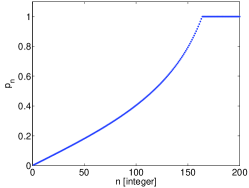
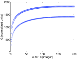
Figure 2: The left panel displays $p_{n}$ for a system with $\alpha=0.7$ and $\mathcal{M}=200$ open modes. The crosses in the right panel are for the cumulative sum over $(1-p_{n})/p_{n}$. The circles are calculated from the exact formula. Namely, the matrix $h$ is diagonalized, and the cumulative trace over the square of its elements is displayed.

We now turn to the calculation of the conductance. First of all, let us calculate the Landauer conductance. Thanks to the simple structure of the $g^{T}_{nm}$ matrix, the calculation is quite easy

$$G_{\mbox{\tiny Landauer}}=\frac{e^{2}}{2\pi\hbar}\sum_{n,m}g^{T}_{nm}=\frac{e^{2}}{2\pi\hbar}\sum_{n}g_{n}$$ (67)

Each channel has total transmission in the range $(1/2)<g_{n}<1$ and therefore the conductance (in normalized units) roughly equals to the number of open modes. Substitution of (64) leads to:

$$G_{\mbox{\tiny Landauer}}=\frac{e^{2}}{2\pi\hbar}\sum_{n}(1-(p_{n}/2))=\frac{e^{2}}{2\pi\hbar}[1-\frac{1}{4}\alpha+\mathcal{O}(\alpha^{4})]\mathcal{M}$$ (68)

For the multimode conductance of Eq.(3) the calculation is more complicated. At first sight it seems that the calculation should be done numerically as in Fig. 2. The numerical calculation in Fig. 2 (circles) is done in a way which is inspired by a similar type of calculation within the Landauer formalism. We define $h_{nm}=([2g^{T}/(1-g^{T}+g^{R})]_{nm})^{1/2}$ and write the sum in Eq.(3) as $\mbox{trace}\left[h^{{\dagger}}h\right]$. Then we make singular value decomposition of $h$ and sum over the squares of its eigenvalues.

The other way to calculate the multimode conductance starts with an attempt to make a zero order evaluation of the sum. This means setting $c=0$ in Eq.(63). The resulting estimate gives a rough approximation as seen from Fig.2 (crosses). The main source of error are evidently the low modes. Surprisingly it turns out that the calculation can be carried out to infinite order in $c$, thanks to miraculous cancellations. Using the expansion

$$\frac{1}{A-cB}=\frac{1}{A}+c\frac{1}{A}B\frac{1}{A}+c^{2}\frac{1}{A}B\frac{1}{A}B\frac{1}{A}+...$$ (69)

with $A_{nm}=p_{n}\delta_{nm}$ and $B_{nm}=(1/2)p_{n}p_{m}$, we get the result

$$\left[\frac{1}{1-g^{T}}\right]_{nm} = \frac{1}{p_{n}}\delta_{nm}+(c/2)\frac{1}{p_{n}}p_{n}p_{m}\frac{1}{p_{m}}+$$ (70)

$$+ (c/2)^{2}\sum_{k}\frac{1}{p_{n}}p_{n}p_{k}\frac{1}{p_{k}}p_{k}p_{m}\frac{1}{p_{m}}+...=\frac{1}{p_{n}}\delta_{nm}+c$$

where in the last step we have made a geometric summation over all orders. Now we can calculate the conductance

$$G=\frac{e^{2}}{2\pi\hbar}\sum_{n,m}\left[\frac{g^{T}}{1-g_{T}}\right]_{nm}=\frac{e^{2}}{2\pi\hbar}\left[\left(\sum_{n}\frac{1}{p_{n}}\right)+c\mathcal{M}^{2}-\mathcal{M}\right]$$ (71)

Recall that $c=1/\sum_{n}p_{n}$. Hence this expression requires merely the evaluation of the sums $\sum_{n}p_{n}$ and $\sum_{n}(1/p_{n})$. If we have $p_{n}\approx 1$ for all modes, then we get simply $G=(e^{2}/(2\pi\hbar))\mathcal{M}$ which reflects that number of open modes. But the interesting case is when $\alpha$ is small:

$$G\approx\frac{e^{2}}{2\pi\hbar}\left[\frac{1}{\alpha}(1+\ln(2\mathcal{M}))-1+\mathcal{O}(\alpha)\right]\mathcal{M}$$ (72)

Unlike the case of the Landauer conductance, the result does not reflect the number of open modes. The contribution of the low modes is singular in the limit of small $\alpha$. Furthermore, the conductivity (conductance per channel) diverges logarithmically in the classical limit.

15 Concluding remarks

Much of the derivations in this paper can be generalized to analyze “quantum pumping”. In Ref.[21] we have considered a single mode device where the current is induced by translating a scatterer. Namely, $\mathcal{I}=-G\dot{X}$ and hence the transported charge is $dQ=-GdX$ where $dX$ is the displacement of the scatterer. From the BPT formula one obtains

$$G\ =-(1-g_{0})\times\frac{e}{\pi}k_{\mbox{\tiny F}}$$ (73)

where $g_{0}$ is the transmission of the scatterer and $k_{\mbox{\tiny F}}$ is the Fermi momentum. If we close the system into a ring, and use the same assumptions as in this paper we get

$$G=-\left[\frac{1-g_{0}}{g_{0}}\right]\left[\frac{g_{T}}{1-g_{T}}\right]\times\frac{e}{\pi}k_{\mbox{\tiny F}}$$ (74)

where $g_{T}$ is the overall transmission of the device. Multi-mode generalizations of these results can be obtained by employing either the Kubo or the Master equation approach as in the present paper (not published).

We regard the “Ohmic” problem that has been discussed in the present paper, and the above mentioned “pumping” problem of Ref.[21], as the prototype models for the application of linear response theory: The “Ohmic” problem has to do with the dissipative part of the response, while the “pumping” problem has to do with the geometric (non-dissipative) part of the conductance matrix. In both cases we can use the Kubo formalism as a starting point, and in both cases we can regard the scattering approach (Landauer-BPT) as a special limiting case. However, one should be aware of the subtle differences between the two problems. The main point to remember is that the adiabatic limit of “quantum pumping” is the non-vanishing “adiabatic transport” formalism, while the adiabatic limit of the “Ohmic” problem gives zero conductance. For further details see [5].

We have assumed that the coherence time is short compared with the time that it takes to encircle the ring. This makes the calculation insensitive to the energy $E$. Once we consider a strictly isolated system, we get an $E$ dependence that has to do with semiclassical energy scales such as $(\hbar/L)v_{F}$. Such energy scales are larger compared with the mean level spacing ($\propto\hbar^{d}$), and may invalidate the Kubo formalism. An extreme example for the implication of having a non-universal energy scale is analyzed in in Ref.[14]. The study of the general multi-mode case introduces further conceptual as well as technical complications [15].

References

References

- [1] S. Datta, Electronic Transport in Mesoscopic Systems (Cambridge University Press 1995).
- [2] Y. Imry, Introduction to Mesoscopic Physics (Oxford Univ. Press 1997), and references therein.
- [3] M. Büttiker et al, Z. Phys. B-Condens. Mat., 94, 133 (1994). P. W. Brouwer, Phys. Rev. B58, R10135 (1998).
- [4] D. Cohen, Phys. Rev. B 68, 201303(R) (2003).
- [5] For mini-review and further references see: D. Cohen, “Quantum pumping and dissipation in closed systems”, Proceedings of the conference “Frontiers of Quantum and Mesoscopic Thermodynamics” (Prague, July 2004), to be published in Physica E. http://www.bgu.ac.il/dcohen/ARCHIVE/pme.pdf.
- [6] M. Buttiker, Y. Imry and R. Landauer, Phys. Lett. 96A, 365 (1983).
- [7] R. Landauer and M. Buttiker, Phys. Rev. Lett. 54, 2049 (1985). M. Buttiker, Phys. Rev. B 32, 1846 (1985).
- [8] Y. Imry and N.S. Shiren, Phys. Rev. B 33, 7992 (1986).
- [9] Y. Gefen and D. J. Thouless, Phys. Rev. Lett. 59, 1752 (1987).
- [10] A. Kamenev and Y. Gefen, Int. J. Mod. Phys. B9, 751 (1995).
- [11] B. Reulet M. Ramin, H. Bouchiat and D. Mailly, Phys. Rev. Lett. 75, 124 (1995).
- [12] M. Wilkinson, J. Phys. A 21 (1988) 4021.
- [13] M. Wilkinson and E.J. Austin, J. Phys. A 23, L957 (1990).
- [14] D. Cohen, H. Schanz, T. Kottos, cond-mat/0505295.
- [15] In collaboration with M. Wilkinson, B. Mehlig and S. Bandopadhyay
- [16] C. Jarzynski, Phys. Rev. E 48, 4340 (1993).
- [17] D. Cohen, Annals of Physics 283, 175 (2000).
- [18] D. Cohen, Phys. Rev. B 68, 155303 (2003).
- [19] T. Kottos and U. Smilansky. Phys. Rev. Lett. 79, 4794 (1997).
- [20] D. Cohen, unpublished
- [21] D. Cohen, T. Kottos and H. Schanz, Phys. Rev. E 71, 035202(R) (2005).
- [22] I thank Y. Oreg (Weizmann Inst.) and B. Shapiro (Technion Inst.) for discussions that have motivated the clarification of questions that are related to the long time scenario.