Canalizing Kauffman networks: Non-ergodicity and its effect on their critical behavior

Abstract

Boolean Networks have been used to study numerous phenomena, including gene regulation, neural networks, social interactions, and biological evolution. Here, we propose a general method for determining the critical behavior of Boolean systems built from arbitrary ensembles of Boolean functions. In particular, we solve the critical condition for systems of units operating according to canalizing functions and present strong numerical evidence that our approach correctly predicts the phase transition from order to chaos in such systems.

Biological and social systems typically comprise a large number of interacting units coupled through a nontrivial network of interactions. Examples of such systems include the metabolic processes in living cells lee02 and social interactions in human groups wassermann94 ; moreira04 . Remarkably, these systems exhibit a high degree of self-organization that ensures their continued functioning and allows them to respond to environmental changes. A challenging aspect in the study of complex systems is how to model both the diversity of the evolving units and the intricate structure of their interactions amaral04a .

Discrete (agent-based) models are among the most common methods used to tackle this challenge. In particular, Boolean networks kauffman (BNs) have been used to model systems as varied as gene regulation networks kauffman , evolution stern99 , and neuronal networks kurten88 —see aldana03 for a review of BN and their applications. It has been shown that BNs share many common properties with real systems kauffman ; amaral04b , the most remarkable probably being a transition from an ordered to a chaotic phase.

A BN consists of $N$ interacting units whose states $\sigma_{i}$ are binary variables. Each unit $i$ is connected to $k_{i}$ other units and its state is updated according to a specific rule

$$\sigma_{i}(t+1)=F_{i}[\sigma_{i_{1}}(t),\sigma_{i_{2}}(t),...,\sigma_{i_{k_{i}}}(t)],$$ (1)

where $F_{i}$ is a Boolean function, and the $\{\sigma_{i_{j}}\}$ are the states of the units connected to $i$, which may or may not include $i$ itself. Boolean functions are represented by a truth table that lists the output of the function for each of the possible set of input values.For a function with $k$ variables there are $2^{k}$ possible input set, yielding $2^{2^{k}}$ different possible functions.

The ensemble of functions ${\cal E}$ defines the probability with which each function appears in the system. In the original formulation, BNs have the coupling connections chosen at random and the Boolean functions $F_{i}$ drawn from an ensemble ${\cal{E}}_{rand}(\rho)$, where $\rho$ is the fraction of active states in the output of the functions. In the following we will refer to $\rho$ as the “bias”, although the case $\rho=0.5$ is actually unbiased. This instance of the model is usually denoted Kauffman networks or random Boolean networks (RBNs).

Typically, BNs display a transition from order to chaos. In the ordered phase, the network evolves toward limiting cycles and, upon a perturbation, the system usually converges back to the initial limiting cycle. In the chaotic phase, the lengths of the attractor cycles grow exponentially with $N$ and almost any perturbation will drive the system toward a different attractor. The critical behavior of RBNs has been determined by means of several different techniques derrida86 ; luque00 . Not much, however, is known about the critical behavior of BN with other ensembles of functions.

In a recent paper, Shmulevich and Kauffman shmulevich04 suggested that the dynamical behavior of a BN can be related to the “average influence” of the variables of its Boolean functions. Here, we use the concept of damage spreading to demonstrate the role of the influence in the dynamical behavior of BNs. We show that, since BNs are nonlinear models not likely to have ergodic dynamics, a naive average of the influence over the whole phase-space of BNs does not necessarily yield a correct estimate of the effective influence of the Boolean variables. We thus revise the definition of average influence in order to account for the non-ergodicity of the dynamics of BNs. Our definition enables us to derive the critical condition of networks of canalizing Boolean functions, a case of particular biological relevance harris01 ; kauffman03 . Finally, we show numerical evidence that our method correctly predicts the critical condition for networks of canalizing Boolean functions.

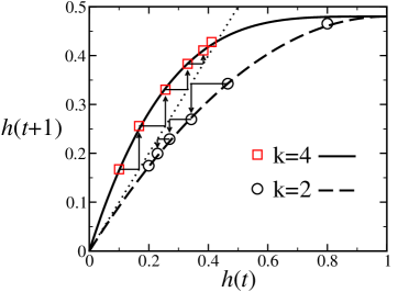
Figure 1: The critical condition for Boolean networks (BN). The Hamming distance $h(t)$ is defined as the normalized difference between two replicas of a BN at time $t$. We show in this figure the iterative mapping for the Hamming distance for the case of random BNs with bias $\rho=0.6$ derrida86 . The solid line corresponds to a network with connectivity $k=4$ and the dashed line to $k=2$. The symbols indicate the Hamming distances obtained numerically for a few time steps in the evolution of two biased networks with $k=4$ and $k=2$. The identity mapping, indicated by the dotted line, and the arrows are included to illustrate the time evolution of $h(t)$. For the case $k=4$, the Hamming distance remains at finite value, while for $k=2$ it tends to zero. The system is in the ordered phase when the Hamming distance converges to zero. Note that, $h=0$ is a fixed point of the mapping, but is unstable whenever the iterative mapping at the origin grows with a steeper slope than the identity line; cf. Eq. (2).

The dynamics of BNs can be quantified by measuring the spread of “damage” through the network. This is done by comparing the parallel evolution of two “replicas” of the system. The replicas have identical Boolean functions and coupling connections, but the initial state of the units in the replicas differs in only a small fraction of the units. The damage, which is also known as the Hamming distance $h(t)$, is defined as the fraction of units that are in different states in the two replicas. If, after some transient time, the evolving replicas are likely to converge to the same state, i.e., $h(t)\to{0}$, then the dynamics of the system is robust with regard to small perturbations, a signature of the ordered phase. If, however, the replicas are likely to never converge, then the dynamics is sensitive to small perturbations to the initial state, a signature of the chaotic phase. As discussed in the caption of Fig. 1, a system is in the ordered phase whenever

$$\left.\frac{dh(t+1)}{dh(t)}\right|_{h(t)\to 0}<1,$$ (2)

Significantly, the susceptibility of unit $i$ to “damage” in its neighbors can be related to the influence of their variables on $F_{i}$. One defines the influence $I_{j}(F_{i})$ of the $j$th variable of a function $F_{i}$ as the probability that the function $F_{i}$ changes its value when the value of $\sigma_{j}$ is changed kahn88 ; lyap . The average influence of a function $I(F_{i})\equiv\frac{1}{k_{i}}\sum_{j}{I_{j}(F_{i})}$, and the average influence $I({\cal E})$ of an ensemble ${\cal E}$ of Boolean functions is $I({\cal E})\equiv\langle{I(F_{i})}\rangle_{\cal{E}}$, where $\langle{...}\rangle_{\cal E}$ indicates an average over the ensemble ${\cal{E}}$.

One can generalize this definition to multiple variables kahn88 : $I^{(1)}\equiv I$ is the average influence of one variable, $I^{(2)}$ is the average influence of two variables, and so on. The probability that an arbitrary unit is damaged in the next step depends on the number $k_{d}$ of damaged inputs it gets and on the influence $I^{(k_{d})}$ of $k_{d}$ variables. Since the inputs are an arbitrary sample of the entire network we can assume that $k_{d}$ follows a binomial distribution and write the evolution of the Hamming distance as

$$h(t+1)=\sum_{k_{d}=1}^{k}{I^{(k_{d})}\left(k\atop k_{d}\right)[h(t)]^{k_{d}}[1-h(t)]^{k-k_{d}}}$$ (3)

where $\left(k\atop i\right)$ is the binomial coefficient. Thus, the influences $I^{(k_{d})}$ determine the shape of the iterative mapping of $h(t)$. Inserting Eq. (3) into Eq. (2), we have that the critical condition depends only on the average influence of one variable,

$$I({\cal{E}},k_{c})k_{c}=1.$$ (4)

Equation (4) enables us to determine the critical condition for BNs with arbitrary ensembles of functions sdk .

This is not trivial, however. The difficulty in using Eq. (4) lies in computing the influence of the variables of the Boolean functions present in the network. In principle, the influence of the variables can be determined by counting in the truth table the number of times that by changing the value of only one variable results in a change in the value of $F$. This approach, which was explored in shmulevich04 , implicitly assumes ergodicity, that is, all inputs can arise with the same probability during evolution, and time average over the states visited by the network yields the same result as average over the whole phase-space. This is an implausible assumption which is unlikely to hold for the dynamics of arbitrary BNs.

In some instances, however, an equaly weighted average does yield to correct results. An example is the ensamble of RBNs luque00 . Note that this does not imply that RBNs are ergodic. In fact, the dynamics of BNs in general converge to limiting cycles that occupy only a fraction of the entire phase-space. To correctly average the influence of the Boolean variables, one must measure the influence only on those states composing the limiting cycles.

We can verify in which cases an equally weighted average can work. If one assumes that the states of the neighbors of a unit are not correlated with the state of the unit it self (random-graph approximation), it follows that the input acting on the unit is a statistical sample of the whole network. Thus, the probability of a certain input depends on the fraction $q$ of units that are in the active state. That is, if the network has a bias toward activity, $q>0.5$, the inputs with more 1s will be more frequent than the inputs with more 0s. Therefore, the activity $q$ of the network should be taken into account when computing the average influence of the BN. The reason why a simple average over the whole phase-space works in RBNs and a few other ensambles is that, on these networks, the influence does not depend on $q$, thus, averaging over the states of the limiting cycles yields the same result as averaging over the whole phase-space. As we will demonstrate later, this property does not generally hold for arbitrary ensembles of Boolean functions.

In the following, we focus on the ensemble of canalizing Boolean functions ${\cal E}_{can}$. Studies of gene regulation in eukaryots have showed that the Boolean idealization is a good approximation for the non-linear dynamics of this system and that the gene regulating mechanisms have a strong bias toward canalizing functions harris01 . A Boolean function is canalizing if whenever one variable, the canalizing variable, takes a given value, the canalizing value, the function always yields the same output. The ensemble of canalizing functions can be separated into four mutually exclusive classes of functions:

$$F(\sigma_{1},\sigma_{2},...)= \sigma_{1} G(\sigma_{2},...),$$ OR (5a)

$$F(\sigma_{1},\sigma_{2},...)= ( \sigma_{1}) G(\sigma_{2},...),$$ NOTAND (5b)

$$F(\sigma_{1},\sigma_{2},...)= ( \sigma_{1}) G(\sigma_{2},...),$$ NOTOR (5c)

$$F(\sigma_{1},\sigma_{2},...)= \sigma_{1} G(\sigma_{2},...),$$ AND (5d)

where $\sigma_{1}$ is the canalizing variable, “AND,” “OR,” and “NOT” are the logical Boolean operators, and $G$ is the non-canalizing part of the function that carries the dependence on the remaining variables. Each of this classes represents a different type of regulation. The class described by (5a) represents “sufficient activators,” that is, $\sigma_{1}=1$ is sufficient to assure an active state for the unit. The class described by (5b) represents “sufficient repressors,” that is, $\sigma_{1}=1$ always results in an inactive state for the unit. The classes described by (5c) and (5d) represent “necessary repressors” and “necessary activators,” respectively. In these cases, $\sigma_{1}=0$ is also enough to determine the output of the function.

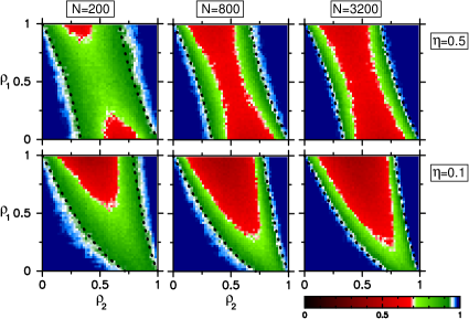
Figure 2: Order-chaos phase-transition for networks of canalizing Boolean functions. The color coding represents the probability that, after changing the state of a random unit of a network in a limiting cycle, the system returns to the same cycle. The resilience of the network to small perturbations is a signature of the ordered phase. The parameter $\eta$ gives the probability with which a Boolean function in the network is canalized by an active input. In the trivial case $\eta=0.5$, the average influence does not depends on the activity of the network and the influence can be computed with an average over the truth table of the Boolean functions in the network, and one finds the critical condition when $kI=1$ in Eq. (9). In the non-trivial case $\eta=0.1$ one finds no difference in the value of the influence when computed from the truth table of the functions. However, it is clear that the critical curve is sensible to the value of $\eta$. The difference is due to the fact that in the latter case the average influence depends on the activity of the network and one has to make a weighted average over the states occupied by the limiting cycles and the critical condition is $kI=1$ in Eq. (8). In both cases, as the network grows, the transition becomes sharper and approaches the critical curves (dotted lines).

The average influence for the ensamble ${\cal{E}}_{can}$ depends on the probability $P_{can}$ with which $\sigma_{1}$ takes the canalizing value. For classes described by (5a) and (5b), $\sigma_{1}$ gives a sufficient condition for activation or repression respectively. This means that for these classes the canalizing value is an active state. On other hand, for classes (5c) and (5d) the canalizing value is an inactive state. If both cases are equally present on the network, one has always $P_{can}=0.5$. However, if one of the canalizing values is more frequent than the other, $P_{can}$ will depend on the fraction $q$ of units in the active state. To account for this effect we define $\eta$ as the fraction of the functions in the ensemble that fall into classes (5a) and (5b). Thus, the probability that the canalizing variable takes the canalizing value is

$$P_{can}=q\eta+(1-q)(1-\eta).$$ (6)

The next step is determining the average activity $q$ of the network when the limiting cycles are reached. To do this, we need to define some relevant parameters characterizing the ensemble of canalizing functions. Note that, for the classes described by Eqs. (5a) and (5c), the use of the “OR” operator means that the values of $\sigma_{1}$ and $G$ give two alternative conditions yielding an active output, while for the classes described by Eqs. (5b) and (5d), the “AND” operator means that the values of $\sigma_{1}$ and $G$ give two necessary conditions for obtaining an active output. The use of the “OR” operator thus results in a bias toward activity. To quantify this bias, we define $\rho_{1}$ as the fraction of the functions in the ensemble that fall into classes (5a) and (5c). Note that, the bias of the canalizing functions toward the active state will also depend on $G$, the non-canalizing part of $F$. We assume that $G$ is chosen as a random Boolean function with bias $\rho_{2}$.

It is possible to measure the probability that a random input results in an active output. This probability is the average bias $\rho_{can}=(\rho_{1}+\rho_{2})/2$ of the ensemble of canalizing functions ${\cal{E}}_{can}$. However, one can not assume that in the limiting cycles any input happen with the same chance. For the ensemble ${\cal{E}}_{can}$, the average activity for the limiting cycles is given by

$$q=\rho_{1}P_{can}+\rho_{2}(1-P_{can}),$$ (7)

where the first term on the right accounts for the probability that the function is being canalized to activity and the second for the probability that the function $G$ is driving the function to activity.

We can now proceed and calculate the average influence for the ensemble of canalizing functions. We will consider first only the average influence of the canalizing variable $I_{1}$, which is given by the probability that $G=0$ when the OR operator is chosen, plus the probability that $G=1$ when the AND operator is chosen; $I_{1}=\rho_{1}(1-\rho_{2})+(1-\rho_{1})\rho_{2}$. The influence of the remaining variables $I_{i}$ depends on the probability that the functions are not locked by the canalizing variable, $1-P_{can}$, and on the bias $\rho_{2}$ of $G$. Finally, we have $I_{i}=2\rho_{2}(1-\rho_{2})(1-P_{can})$, and:

$$kI=\rho_{1}+\rho_{2}-2\rho_{1}\rho_{2}+2\rho_{2}(1-\rho_{2})[\eta+q(1-2\eta)](k-1).$$ (8)

If one assumes that all inputs in the truth table contribute with the same weight to the average, then $P_{can}=0.5$, and

$$kI=\rho_{1}+\rho_{2}-2\rho_{1}\rho_{2}+(k-1)\rho_{2}(1-\rho_{2}).$$ (9)

One of the cases where Eq. 9 works is when $\eta=0.5$.

We next test our theoretical results against numerical simulations of BNs of canalizing functions. This is done by building random networks with Boolean functions obeying the ensemble of canalizing functions described by Eq. (5). We assign random initial states to the networks and let them evolve until they reach a limiting cycle weight . We then make a perturbation by changing the state of one of the units in the network. The resilience of the system to this “damage” is the probability that, after the perturbation, the system converges back to the initial limiting cycle estim . We show in Fig. 2 that, as the system size grows, the transition from order to chaos becomes sharper and approaches a critical condition where $kI=1$; cf. Eq. (8).

Note that, when the network has a bias in the canalizing value, $\eta=0.1$, there is a considerable reduction in the region occupied by the chaotic phase, mainly in the region where the network is biased to the inactive state: low $\rho_{1}$ and $\rho_{2}$. This bias for an inactive canalizing value was observed in the mechanisms of gene regulation kauffman03 where the transcription of a given gene may depend on the presence of several activator proteins, that is, a single inactive input—the absence of the one of the activators—can result in an inactive state—no transcription.

The major finding of this study is that, by using the concepts of influence of Boolean variables and damage spreading, we are able to obtain the critical behavior of Boolean networks built from arbitrary ensembles of functions. We show that for most networks the effective influence of the variables cannot be obtained by a simple average over the truth table of the functions. We further obtain an expression for the influence of the variables for networks of canalizing Boolean functions and present strong numerical evidence that our method can accurately predict the critical transition for these networks. Our work suggests that the approach described here can solve the critical transition of other ensembles of Boolean functions such as nested canalizing functions kauffman03 —which are thought to be a valuable model for the description of gene regulation networks—or random threshold functions kurten88 —a common model for neural networks.

We thank A. Díaz-Guilera, L. Guzmán-Vargas, D. B. Stouffer, M. Sales, and R. Guimerà for fruitful discussions. LANA thanks the support of a Searle Leadership Fund Award and a NIH/NIGMS K-25 award.

References

- (1) T. I. Lee et. al., Science 298, 799 (2002).
- (2) S. Wassermann and K. Faust, Social Network Analysis (Cambridge University Press, Cambridge, 1994).
- (3) A. A. Moreira, A. Mathur, D. Diermeier, and L. A. N. Amaral, Proc. Nat. Acad. Sci. USA 101, 12085 (2004).
- (4) L. A. N. Amaral and J. M. Otino, Europ. Phys. J. B 38, 147(2004)
- (5) S. A. Kauffman, J. Theor Biology 22, 437 (1969); The Origins of Order (Oxford University Press, Oxford, 1993).
- (6) M. D. Stern, Proc. Nat. Acad. Sci. USA 96, 10746 (1999).
- (7) K. E. Kürten, J. Phys. A 21, L615 (1988).
- (8) M. Aldana, S. Coppersmith, and L. P. Kadanoff, in Perspectives and Problems in Nonlinear Science, E. Kaplan, J. E. Marsden, and K. R. Sreenivansan, Eds. (Springer Verlag, New York, 2003), http://arxiv.org/abs/nlin/0204062.
- (9) L. A. N. Amaral, A. Díaz-Guilera, A. A. Moreira, A. L. Goldberger, and L. A. Lipsitz, Proc Nat. Acad. Sci. USA 101, 15551 (2004).
- (10) B. Derrida and Y. Pomeau, Europhysics Letters 1, 45 (1986); H. Flyvbjerg, J. Phys. A 21, L955 (1988).
- (11) B. Luque and R. V. Solé, Physica A 284, 33 (2000),
- (12) I. Shmulevich and S. A. Kauffman, Physical Review Letters 93, 048701 (2004).
- (13) S. E. Harris, B. K. Sawhill, A. Wuensche, and S. Kauffman, Complexity 7, 23 (2001).
- (14) S. Kauffman, C. Petersen, B. Samuelsson, and C. Troein, Proc Nat. Acad. Sci. USA 100, 14796 (2003).
- (15) J. Kahn, G. Kalai, and N. Linial, in Proceedings of the 29th Annual Symposium on Foundations of Computer Science (IEEE Computer Society Press, Washington, DC, 1988).
- (16) The concept of influence is related to Boolean derivatives and Lyapunov exponents of BNs luque00 and to the activity defined in shmulevich04 .
- (17) This critical condition can be generalized to the case where the number of variables of the units is drawn from a distribution , becoming .
- (18) In this way, the mean values we obtain represent a weighted average where each attractor is weighted by the size of its basin of attraction.
- (19) Our estimate is obtained by averaging over different instances of the network for each set of parameter values.