Dynamics and Kinetic Roughening of Interfaces in Two-Dimensional Forced Wetting

Abstract

We consider the dynamics and kinetic roughening of wetting fronts in the case of forced wetting driven by a constant mass flux into a 2D disordered medium. We employ a coarse-grained phase field model with local conservation of density, which has been developed earlier for spontaneous imbibition driven by a capillary forces. The forced flow creates interfaces that propagate at a constant average velocity. We first derive a linearized equation of motion for the interface fluctuations using projection methods. From this we extract a time-independent crossover length $\xi_{\times}$, which separates two regimes of dissipative behavior and governs the kinetic roughening of the interfaces by giving an upper cutoff for the extent of the fluctuations. By numerically integrating the phase field model, we find that the interfaces are superrough with a roughness exponent of $\chi=1.35\pm 0.05$, a growth exponent of $\beta=0.50\pm 0.02$, and $\xi_{\times}\sim v^{-1/2}$ as a function of the velocity. These results are in good agreement with recent experiments on Hele-Shaw cells. We also make a direct numerical comparison between the solutions of the full phase field model and the corresponding linearized interface equation. Good agreement is found in spatial correlations, while the temporal correlations in the two models are somewhat different.

1 Introduction

The dynamics and roughening of moving interfaces in a disordered medium is a subject of intense interest in non-equilibrium statistical physics [1]. Examples where such processes are relevant include thin film deposition [2], slow combustion fronts in paper [3], fluid invasion in fractals [4] and porous media [5, 6, 7], and wetting and propagation of contact lines [8, 9, 10]. The understanding of the underlying physics involved in interface roughening is crucial to the control and optimization of these processes, with immediately apparent technological importance. Progress in the theoretical study of interface dynamics has been made over the last two decades and a number of theories have been developed [1, 7] which agree with the experimental findings in some cases. Much of the theoretical work has been based on analyzing (spatially) local interface equations, such as the celebrated Kardar-Paris-Zhang (KPZ) equation [11], where the physics is governed by a (nonlinear) partial differential equation which couples the interface locally with itself and the quenched randomness. However, in many cases such a description is not possible [4, 12].

A particularly important class of problems in the field of kinetic roughening where local theories cannot provide a complete description are those involving fluid invasion in porous media, which are often experimentally studied using Hele-Shaw cells [13, 14, 15, 16] or even paper as the wetting medium [17, 18, 19, 20]. The reason for this is that if the transport of liquid to the advancing wetting front from the reservoir is neglected as in local theories, slowing down of the front in spontaneous imbibition of water in paper cannot be explained by local theories unless the liquid conservation law is included in some artificial way. To properly describe the dynamics of wetting fronts in random medium is a challenging task, and there are several recent theoretical attempts to this end [15, 21, 22]. In particular, in Refs. [12, 24, 23, 25] Dube et al. developed a phase-field model explicitly addressing the issue of liquid conservation in the wetting of a random medium. This is achieved by a generalized Cahn-Hilliard equation with suitable boundary condition which couples the system to the reservoir. A variant of the sharp interface projection method [26, 27] was used to analytically obtain a non-local interface equation for the case of spontaneous imbibition, and from it a new time dependent length scale governing the kinetic roughening $\xi_{\times}\sim t^{1/4}$, was extracted. In Refs. [12, 23] the kinetic roughening of 2D wetting fronts was also analyzed, and estimates for the corresponding scaling exponents were obtained. Furthermore, in a recent comprehensive review paper [28] the case of forced wetting in 2D was briefly discussed, and in Ref. [29] forced wetting in a 3D model of paper was also considered.

In the present work our aim is to carry out a comprehensive analysis of wetting fronts in 2D in the case of forced wetting. To this end, we use the phase-field model of Ref. [12] with boundary conditions corresponding to a constant mass flux at the reservoir boundary. This makes the wetting fronts move at a constant average velocity, in contrast to the Washburn law for spontaneous wetting. We first expand on the standard projection method to make it usable under constant flow boundary conditions, and derive the linearized interface equations corresponding to the forced case. Analysis of these equations reveals a crossover length scale $\xi_{\times}$, which is time-independent in contrast to the spontaneous wetting case [12], and depends on the interface velocity as $\xi_{\times}\propto v^{-1/2}$. It separates two regimes of dissipative behavior and governs the kinetic roughening of the interfaces by giving an upper cutoff for the correlation length of the interface fluctuations. By numerically integrating the phase field model, we find that the interfaces are superrough with a roughness exponent of $\chi=1.35\pm 0.05$, and a growth exponent of $\beta=0.50\pm 0.02$. These results are in good agreement with recent experiments on Hele-Shaw cells [14]. We also make a direct numerical comparison between the solutions of the full phase field model and the corresponding linearized interface equation. Good agreement is found in spatial correlations, while the temporal correlations in the two models are somewhat different.

This paper proceeds as follows: In Section 2 we define the phase field model, and present results from the projection and linearization procedure. We present the resulting interface equations, as well as discuss how the crossover length scale $\xi_{\times}$ emerges. In Section 3 we present our numerical results for the driven interfaces in disordered medium. We consider both spatial and temporal correlation functions, as well as compare the numerical results from the linearized interface equation to the phase field model. Finally, we present our discussion and conclusions in Section 4. The Appendices A and B contain some technical details on the projection and linearization procedures leading to the interface equations.

2 Model for Wetting

2.1 Definition of the Phase Field Model

The model describes the dynamics of a liquid invading a disordered medium at a coarse-grained level. A phase field is used to describe the “wet” and “dry” phases, with a free energy functional such that the dimensionless phase field obtains the values $\phi=+1$ and $\phi=-1$ at the wet and dry phases, respectively. Since the phase field is an effective density field it is locally conserved. Energy cost for an interface is added by the standard coarse-grained gradient squared term. The interaction energy between the random medium and the invading liquid is represented by a quenched random field linearly coupled to the phase field. This leads to the free energy density [12]

$$\mathcal{F}[\phi(\mathbf{x},t)]=\frac{1}{2}(\nabla\phi(\mathbf{x,t}))^{2}+V(\phi(\mathbf{x,t}))-\alpha(\mathbf{x})\phi(\mathbf{x},t),$$ (1)

where $V$ has two minima at $\phi=-1$ and $\phi=+1$, and $\alpha$ is the quenched random field. The standard Ginzburg-Landau form is chosen for $V$, i.e. $V(\phi)=-\phi^{2}/2+\phi^{4}/4$ [12], and the quenched field obeys the relations

$$\langle\alpha(\mathbf{x})\rangle = 0$$ (2)

$$\langle\alpha(\mathbf{x})\alpha(\mathbf{x}^{\prime})\rangle = (\Delta\alpha)^{2}\delta(\mathbf{x}-\mathbf{x}^{\prime}).$$ (3)

The case of positive (negative) $\langle\alpha(\mathbf{x})\rangle$ corresponds to the liquid spontaneously wetting (dewetting) the medium for the case of no external driving [12].

The equation of motion for the conserved phase field is given by the continuity equation $\partial_{t}\phi=-\nabla\cdot\mathbf{j}$ and Fick’s law $\mathbf{j}=-\nabla\mu$, where $\mu=\delta\cal{F}/\delta\phi$. The result is

$$\partial_{t}\phi({\bf x},t)=\nabla^{2}\mu({\bf x},t)=\nabla^{2}\left[-\phi({\bf x},t)+\phi^{3}({\bf x},t)-\nabla^{2}\phi({\bf x},t)-\alpha({\bf x})\right],$$ (4)

which is essentially the Cahn-Hilliard equation [30]. Note that dimensionless units have been set such that the constant relating the phase field gradient to the free energy and the mobility in Fick’s law are both unity. This fixes the choice of units in Eq. (4).

In Refs. [12, 24] the case of spontanous, capillary driven wetting was modeled with Eq. (4) using boundary conditions where the chemical potential was set to a constant at the liquid reservoir $y=0$. In order to model the experimental setup of driving the liquid from the reservoir, we define our phase-field in the half-plane $\{\mathbf{x}|y\geq 0\}$, and at the line $y=0$ impose the boundary condition $\nabla\mu=-F\hat{y}$, where $\hat{y}$ is the unit vector, and $F$ is a constant (flux) parameter (see Fig. 1(a)). On the top end of the system we set $\phi(y\rightarrow\infty)=-1$, and use periodic boundaries in the $x$ direction. Physically this corresponds to driving the liquid via a constant mass flow, leading to an interface propagating at a constant average velocity [28].

The initial condition for the phase field is given by a step function at some height $H(0)=H(t=0)$, $\phi(\mathbf{x},t=0)=1-2\Theta(y-H(0))$. $H(0)$ is also a parameter in our model, but with the gradient boundary condition here its value is irrelevant, in contrast to the case of spontaneous imbibition, where $H(0)$ defines the initial average velocity of the interface [12].

2.2 Linearized interface equation

The quenched disorder field $\alpha(\mathbf{x})$ will cause an initially flat interface to kinetically roughen when it propagates as the liquid invades the medium. A key step in understanding the physics of this process is writing an equation of motion for the 1D single-valued height variable $H(x,t)$, defined conveniently by the condition $\phi(x,H(x,t))=0$ as shown in Fig. 1(a). It is not obvious a priori that this can be done, since the problem is inherently non-local due to the conservation law [12], but it has been shown in Refs. [12] that this can be done using methods discussed in Refs. [26, 31, 32]. In Appendix A we will discuss some technical details of the derivation. The main idea is to use the relevant Green’s function of the problem defined by

$$\nabla^{2}G(x,y|x^{\prime},y^{\prime})=\delta(x-x^{\prime})\;\delta(y-y^{\prime}),$$ (5)

with appropriate boundary conditions. This leads to the integro-differential equation of motion

$$2\int_{-\infty}^{\infty}dx^{\prime}\;G(x,H(x,t)|x^{\prime},H(x^{\prime},t))\;\frac{\partial H(x^{\prime},t)}{\partial t}=\alpha(x,H(x,t))+\sigma\kappa+\Lambda|_{y=H(x,t)},$$ (6)

where $\kappa$ is the interface curvature, and $\Lambda$ is the boundary term, which is non-vanishing for inhomogenous boundary conditions. Note that Eq. (6) holds for any geometry given the appropriate Green’s function. For the half plane with von Neumann boundary condition at $y=0$, the 2D Green’s function is obtained by image charge method as

$$G(x,y|x^{\prime},y^{\prime})=\frac{1}{4\pi}\ln\left[((x-x^{\prime})^{2}+(y-y^{\prime})^{2})((x-x^{\prime})^{2}+(y+y^{\prime})^{2})\right].$$ (7)

The next step towards an explicit interface equation is to linearize in fluctuations around the disorder-free system solution, $H(x,t)=H_{0}(t)+h(x,t)$, and transform to Fourier space, where the equations of different modes of fluctuation are decoupled. The half plane Green’s function defined in Eq. (7) is not square integratable, however, and thus it does not have a Fourier representation. However, we have found that we can avoid this problem by considering a finite strip of width $L$ where $0\leq x\leq L$, and derive a linearized equation of motion for the discrete Fourier modes of the fluctuations. Then we can take the limit $L\rightarrow\infty$ to obtain the equation of motion in Fourier space for an interface in half-plane geometry, and the end result is well-defined. This procedure is exposed in some detail in Appendix B.

The linearization procedure, by construction, gives a separate equation of motion for the mean interface position $H_{0}(t)$, which turns out to be coupled to all the fluctuation Fourier modes $h_{k}$, while the evolutions of the fluctuation modes are independent of each other. The resulting equations are given by

$$\dot{H_{0}} = \frac{F}{2};$$ (8)

$$\dot{h}_{k}\left(1+e^{-2|k|H_{0}}\right) = |k|\left(-\dot{H}_{0}\;h_{k}\left(1-e^{-2|k|H_{0}}\right)-\sigma k^{2}h_{k}+\eta_{k}(t)\right),$$ (9)

from which we immediately obtain the expected result that

$$H_{0}(t)=\frac{Ft}{2}.$$ (10)

This should be contrasted with the Washburn law $H_{0}(t)\propto t^{1/2}$ in the case of spontaneous wetting [12]. It is interesting to note that the functional form of Eq. (9) for the fluctuations of the interface is similar to the case of spontaneous wetting in Ref. [12], except for some sign changes in the terms. It can be shown that these changes are a direct consequence of the differences between the Green’s functions in the two cases, and they lead to significant differences in the behavior of the fluctuations as will be discussed below.

The most immediate aspect of these equations is that the fluctuation equation is non-local in real space. This is to be expected due to the conservation law [12]. The locality of the interface equation in Fourier space owes to the fact that it has been linearized. The interface configuration couples to the disorder in a fundamentally non-linear manner, a fact that is somewhat obscured by the superficially simple form of the disorder term $\eta_{k}$, which is defined as

$$\eta_{k}(t)\equiv\int dx\leavevmode\nobreak\ e^{-ikx}\alpha(x,H(x,t))$$ (11)

The moments of $\eta_{k}$ averaged over disorder realizations thus couple to the interface configuration realizations, which in turn are defined by the disorder. This makes the analysis of $\eta_{k}$ a formidable task that must be solved self-consistently involving the interface equation. In more explicit terms, in expressions such as $\langle\alpha(x,H(x,t))\alpha(x^{\prime},H(x^{\prime},t^{\prime}))\rangle$, the angular brackets denote averages over different realizations of $H$, and results can only be obtained numerically.

In Eq. (9) there are two terms that dissipate fluctuations corresponding to different physical effects: the surface tension term $\sigma k^{3}h_{k}$ and the liquid transport (conservation law) $|k|\dot{H}_{0}\left(1-e^{-2|k|H_{0}}\right)h_{k}$. The surface tension dominates when $k\dot{H_{0}}\ll\sigma k^{3}$, leading to a time independent crossover length scale between the two terms given by

$$\xi_{\times}=2\pi\sqrt{\frac{\sigma}{\dot{H}_{0}}}=2\pi\sqrt{\frac{2\sigma}{F}}.$$ (12)

This is in striking contrast to the spontaneous case, where the corresponding crossover length is time dependent with $\xi_{\times}\propto t^{1/4}$ [12]. Moreover, in the dispersion relation of the fluctuations there is an additional crossover in the transport term obtained by comparing the length scales $H_{0}(t)$ and $k$. Namely, for $kH_{0}(t)\gg 1$ the transport term is $k\dot{H}_{0}$, while for $kH_{0}(t)\ll 1$ it is $2k^{2}H_{0}\dot{H}_{0}$, leading to a crossover between $\omega\propto k$ and $\omega\propto k^{2}$ in the dispersion relation of the interface fluctuations. Regardless of the magnitude of $kH_{0}(t)$, we will show through numerical studies that the crossover length scale $\xi_{\times}$ controls the kinetic roughening of the interface in analogy to the spontaneous imbibition case, in that it defines an upper cut-off for fluctuations that are increasing in time and correlated by the surface tension.

3 Numerical analysis

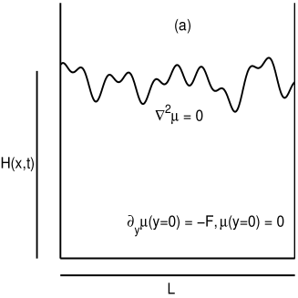
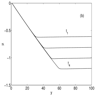
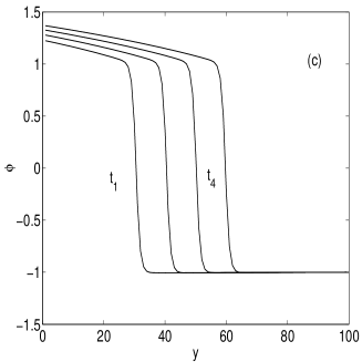
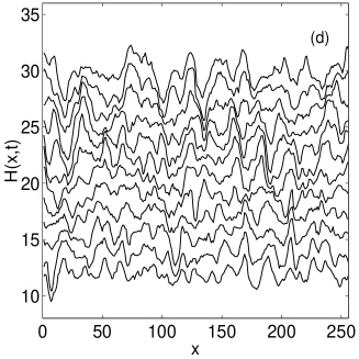
Figure 1: (a) A schematic geometry and setup of the model. The height of the front is described by a single-valued function $H(x,t)$, and the driven boundary condition at the reservoir at $y=0$ is described by a constant gradient of the chemical potential. (b) The profile of the chemical potential $\mu(x,y)$ along the $y$ axis at successive time steps $t_{1}<t_{2}...<t_{4}$. (c) The profile of the density field $\phi(x,y)$ along the $y$ axis at successive time steps corresponding to (b). Note that due to the conservation law these profiles have a finite slope in the wet region of the medium. (d) A set of typical rough front configurations of a rising interface $H(x,t)$ taken at equal time intervals $\Delta t=80$.

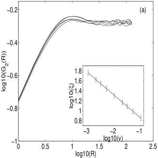
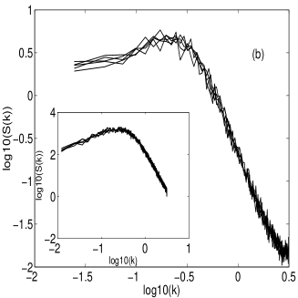
Figure 2: (a) Spatial correlation functions $G_{2}(r,t)$ for a system of size $L=256$, with $\Delta\alpha=0.3$, $v=0.05$ at different times. The data are from $t=10^{3}$ to $t=10^{4}$ at equal time intervals of $t=2\times 10^{3}$. In the inset, the crossover lengths $\xi_{\times}(V)$ obtained from $G_{2}$ for different velocities are plotted. (b) The structure factor $S(k,t)$ plotted against the wave vector $k$ for the same set of parameters as in (a). In the inset, the structure factor obtained from the linearized interface equations is plotted against $k$ for the corresponding set of parameters, except that $L=512$.

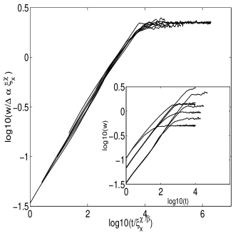
Figure 3: Data collapse of the interface width according to the scaling form of Eq. (16) for different sets of parameters with $L=256$: (i) $\Delta\alpha=0.3$, $v=0.05$ and $0.01$; (ii) $\Delta\alpha=0.2$, $v=0.01,0.005$, and $0.002$; (iii) $\Delta\alpha=0.1$, $v=0.005,0.002$, and $0.001$. The inset shows the original interface width data.

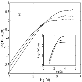
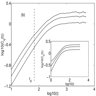
Figure 4: (a) The temporal correlation function $C_{2}(t)$ for $L=256$, with $\Delta\alpha=0.2$ and $v=0.015,0.01$, and $0.005$. In the inset, the corresponding data are shown for the linearized interface equations. (b) Temporal correlation functions $C_{q}(t)$ with $q=2,4$, and $6$ for $L=256$, with $\Delta\alpha=0.2$ and $v=0.015$. In the inset, the the corresponding functions are shown for the linearized interface equations. See text for details.

The interface fluctuations in the presence of quenched disorder were analyzed by numerical integrations of Eq. (4) with the appropriate boundary conditions shown in the schematic representation of Fig. 1. In order to implement the von Neumann boundary condition at $y=0$, Eq. (4) is modified as follows:

$$\partial_{t}\phi({\bf x},t) = \nabla^{2}\left[-\phi({\bf x},t)+\phi^{3}({\bf x},t)-\nabla^{2}\phi({\bf x},t)-FH_{0}(t)-\alpha({\bf x})\right],$$ (13)

where the addition of the term $FH_{0}(t)$ ensures that the interface will propagate at constant velocity $v\equiv\dot{H}_{0}=F/2$ due to the boundary condition $\partial_{y}\mu|_{y=0}=-F$. The above equation is then solved with the Dirichlet boundary condition $\mu|_{y=0}=0$. This is a numerical trick invoked to obtain a chemical potential profile consistent with the von Neumann boundary condition in the domain from the reservoir at $y=0$ to the interface at $y=H$. The position of the interface $H(x,t)$ at each $x$ was defined as $H(x,t)=0$ by linear interpolation between the points of the numerical grid. Without any loss of generality, the chemical potential at the boundary is chosen such that $\mu(x,y=0)=0$, leading to $\phi(x,y=0)=\phi_{0}$, where $\phi_{0}$ is the solution of $-\phi_{0}+\phi_{0}^{3}=FH_{0}(t)$ .

Typical plots for the chemical potential and the density field along the $y$ axis obtained from numerical integration of Eq. (13) without quenched disorder ($\Delta\alpha=0$) are shown in Figs. 1 (b) and (c), respectively. A set of successive interface configurations with $v=0.02$, and $\Delta\alpha=0.2$ are also shown in Fig. 1 (d). It is interesting to note from Fig. 1(c) that behind the moving interface the density field has a finite slope, which remains constant in time. This is due to the underlying local conservation law for $\phi(x,y)$. We note that the slighly growing value of $\phi$ which is greater than $+1$ is just a numerical artifact and can be removed by using a method of moving box to hold the interface at a constant height, i.e. pulling down the disorder field at constant time intervals.

3.1 Spatial roughness

With $\Delta\alpha>0$, the driven wetting front kinetically roughens as can be seen in Fig. 1(d). To characterize the spatial extent of the roughness, we first consider the spatial two-point correlation function

$$G_{2}(r,t)=\langle\overline{[h(x+r,t)-h(x,t)]^{2}}\rangle^{1/2},$$ (14)

which is directly related to the structure factor $S(k,t)\equiv\langle\overline{h_{k}(t)h_{-k}(t)}\rangle$. In the above equations the brackets denote an average over different configurations of random noise, and the overbar a spatial average over the system.

In Fig. 2(a) we show numerical data for the spatial correlation function. We find that the correlation length of the roughness of the interface saturates after an initial growth. According to Eq. (12), the crossover length $\xi_{\times}$ is related to the interface velocity by $\xi_{\times}\sim v^{-1/2}$. In the inset of Fig. 2(a) we plot the velocity dependence of the corresponding crossover length $\xi_{2}$ found from $G_{2}(r)$. We indeed find that this length $\xi_{2}\sim v^{-0.45}$, which means that $\xi_{2}\propto\xi_{\times}$ as in the case of spontaneous wetting, too [12].

An estimate for the global roughness exponent $\chi$ can be obtained from the structure factor $S(k,t)$, as shown in Fig. 2(b). As expected, we find that $S(k)\sim 1/k^{1+2\chi}$ is well satisfied, with a global roughness exponent of $\chi\approx 1.25$, and a crossover to a plateau corresponding to distances larger than the intrinsic correlation length $\xi_{\times}$, consistent with the analysis from the linearized interface equation. We actually found that the global roughness exponent slightly depends upon the velocity and increases with decreasing velocity until asymptotically approaching a value of about $1.35$. For velocities $v=0.005,0.002$, and $0.001$, with $\Delta\alpha=0.1$, it was found that $\chi\approx 1.27,1.35$, and $1.37$, respectively. Moreover, that global roughness exponent slightly depends on the strength of the noise. For example, for $v=0.005$, $\chi\approx 1.27$ and $1.36$ for $\Delta\alpha=0.1$ and $0.2$, respectively. We also compared the crossover lengths obtained from $G_{2}(r,t)$ to those from $S(k,t)$, and found that the value of $\xi_{\times}$ from $S(k,t)$ is about one-half of that from $G_{2}(r,t)$, independent of disorder strength.

We also estimated the the local roughness exponent $\chi_{\textrm{loc}}$ according to the scaling relationship $G_{2}(r=1,t)\sim\xi_{\times}^{\chi-\chi_{\textrm{loc}}}\sim v^{(\chi_{\textrm{loc}}-\chi)/2}$ for different velocities [12], and found that $\chi_{\textrm{loc}}\approx 1.0$, as expected for superrough interfaces. The spatial correlation funnction $G_{2}(r,t)$ should also follow the same scaling form $G_{2}(r,t)\sim\Delta\alpha v^{-\chi/2}g(rv^{1/2})$ as $G_{2}(r,H)$ for spontaneous imbibition with fixed interface front height [12].

3.2 Temporal roughness

To quantify the temporal development of the roughness, we consider the width of the interface defined by

$$w^{2}(t)=\langle\overline{(h(x,t)-\overline{h(x,t)})^{2}}\rangle.$$ (15)

In the presence of quenched disorder the roughness initially increases as a power law of time, as shown in Fig. 3. After a crossover, the roughness reaches a saturated regime. For small $\Delta\alpha=0.1$, only relatively low velocities were studied, because for velocity as high as $v=0.05$, the roughness profile shows pronounced oscillations. The cause of such numerical oscillations was identified to be the numerical interpolation of the interface position between the grid points with time scale equal to lattice size over the velocity. It can be clearly seen from the inset of Fig. 3 that for the same noise strength, all the roughness curves follow the same initial growth profile, suggesting an universal growth exponent $\beta$. It was found that for $\Delta\alpha=0.1,0.2$, and $0.3$, the corresponding values of $\beta$ are about $0.48,0.50$, and $0.52$, respectively.

The saturated width of the interface was found to be independent of the lateral system size as long as the lateral system size is larger than the intrinsic crossover length $\xi_{\times}$, which has been derived from the linearized interface equation in the preceding section. It should be pointed out that in Ref. [28], where the case of driven wetting was briefly discussed, it is claimed that after an initial growth, the interface roughness follows a weak logarithmic growth. From Fig. 3 one can see that we do not find any evidence of such a logarithmic growth regime, although it could be too slow to be detected numerically.

Assuming that the crossover length $\xi_{\times}$ controls the roughening process, we can use the results in Ref. [12] and write a Family-Vicsek type of scaling relation

$$w(t)=\Delta\alpha\xi_{\times}^{\chi}g\left(\frac{t^{\beta}}{\xi_{\times}^{\chi}}\right).$$ (16)

Data collapse using this scaling from is presented in Fig. 3. Using the data collapse, we give our best estimates for the roughness and growth exponents as $\chi=1.35\pm 0.05$ and $\beta=0.50\pm 0.02$. We note that Ref. [28] estimates that $\chi\approx 1.25$ and $\beta\approx 0.4$, with $\beta=\chi/3$. However, our results do not support this relation.

In the case of spontaneous imbibition, it was found that the rough interfaces obey temporal multiscaling, with different scaling exponents for different moments of the time-dependent correlation functions [12]. These functions and the corresponding exponents are defined by

$$C_{q}(t)=\langle\overline{[H(x,t+s)-H_{0}(t+s)-H(x,s)+H_{0}(s)]^{q}}\rangle^{1/q},$$ (17)

for $q=1,2,3,...$. The correlation functions $C_{2}(t)$ are shown in Fig. 4(a) for different velocities. The crossover time $t_{\times}$ between the power law regime of $C_{2}(t)$ and saturation increases with decreasing velocities. The different functions $C_{q}(t)$ for $q=2,4$ and $6$ are shown in Fig. 4(b). At early times all the functions follow power law behavior $C_{q}(t)\sim t^{\beta_{q}}$, with exponents $\beta_{q}\approx 0.94$ which are independent of $q$. This behavior is, however, observed only in time scales smaller than the disorder persistence time $t_{d}=\Delta y/v$, where $\Delta y=1$ is the dimensionless spatial discretization step. If we consider $C_{q}(t)$ for $t>t_{d}$, we find evidence multiscaling with $\beta_{2}\approx 0.79$, $\beta_{4}\approx 0.69$ and $\beta_{6}\approx 0.54$ in a small time regime, similar to the spontaneous case [12]. However, it is difficult to verify true multiscaling here because of the rapid crossover to the saturated regime, although we do expect avalanche type of motion to be present here, which often leads to multiscaling behavior [33].

3.3 Numerical Results from the Linearized Interface Equations

An interesting question concerns the range of validity of the linearized interface equation (LIE), Eq. (9), for the fluctuations of the height, in particular in the driven, nonlinear regime with noise included. This issue is also related to the possible existence of universality classes of roughening for conserved systems with quenched noise; a problem for which there are virtually no analytical results. To this end, we have integrated Eq. (9) numerically in time. To incorporate the nonlinear nature of the disorder $\eta(x,H(x,t))$, a back-and-forth Fourier transformation scheme is required at every time step. A square lattice landscape of independently Gaussian distributed noise was used for $\eta(x,y)$. We note that solving Eq. (9) instead of the full 2D phase field model is numerically much easier.

To compare the results with the phase-field model, we numerically computed the same set of correlation functions. From the analytic derivation of the interface equation, we can obtain a quantitative map between the parameters of the phase field model and the interface model, which is as follows. The interface velocities should obviously be the same. The disorder fields between the models are related by $\eta=M\alpha$, where $M$ is the mobility in Fick’s law. In our dimensionless units $M=1$. The effective surface tension in the phase field model is given by the standard form of the potential $V(\phi)$ as $\sigma_{pf}=\int du\leavevmode\nobreak\ (\partial_{u}\phi_{0}(u))^{2}$, where $\phi_{0}$ is the 1D kink solution of the disorder-free system. The surface tension in the interface equation comes out as $\sigma=M\sigma_{pf}$.

The results from the LIE are collected in the insets of the corresponding phase field results in Figs. 2-4. Obviously, the length scale $\xi_{\times}$ is present in an identical manner in both cases. Remarkably enough, the corresponding results from the two cases are in most cases quantitatively close to each other. There are some important differences, however. First, the saturated interface widths differ by about $20\%$, the interfaces from the LIE being rougher. Since the interface model only takes into account linear dissipation effects, we would expect it to underestimate the stiffness of the interface, leading to larger roughness amplitudes than in the full phase field model.

Next, we examine the data collapse for the interface roughness (Fig. 3) using the scaling function of Eq. (16). The best collapse is obtained for slightly different values of the exponents as compared to the phase-field model. The roughness exponent is close to the previous value, namely $\chi=1.27\pm 0.05$. However, the growth exponent is now given by $\beta=0.37\pm 0.04$ for the LIE, where the difference to the phase field result is outside of the numerical uncertainties. In the LIE we also noted a slight deviation from the behavior of the crossover time $t_{\times}\propto\xi_{\times}^{\chi/\beta}$ as a function of the disorder strength $\Delta\alpha$. Another difference between the two models was found in temporal multiscaling. In the LIE each of the moments increases with a different exponent $\beta_{q}$ even at times smaller than the disorder persistence length $t_{d}$. The exponents are $\beta_{2}=0.75\pm 0.03$, $\beta_{4}=0.55\pm 0.05$, and $\beta_{6}=0.47\pm 0.03$. The values of these exponents are lower than in the phase-field model, which is not surprising since the LIE has a lower value of $\beta$, too.

4 Summary and Conclusions

In the present work, we have studied wetting of a disordered medium driven by a constant mass flux in a 2D system. Our model is a prototype phase field model incorporating mass conservation into the flow of two immiscible fluids, Eq. (4). From this model we have derived non-local interface equations to lowest order in Fourier space fluctuations, Eqs. (8) and (9). Because of the linearization, these equations are local in Fourier space. The constant flux boundary condition gives rise to a interface that moves with a constant velocity proportional to the flux. We have obtained a time-independent crossover length scale $\xi_{\times}\propto\sqrt{\sigma/v}$ from the interface equations. Numerically, we find that the kinetic roughening of an interface is governed by a scaling relation of the Family-Vicsek type, where $\xi_{\times}$ controls the extent of the fluctuations (for $\xi_{\times}<L$) as given by Eq. (16). For the kinetic roughening of the interfaces, we find that they are superrough, with $\chi=1.35\pm 0.05$ and $\chi_{\rm loc}\approx 1$. For temporal roughness, $\beta=0.50\pm 0.02$, and there is numerical evidence of temporal multiscaling for $t>t_{d}$. We note that all these results are in qualitative but not in quantitative agreement with the case of spontaneous imbibition studied earlier in Refs. [12] for interfaces, which are kept at constant height in the steady-state regime described by Washburn’s law.

In addition to obtaining the LIE by analytic methods, we have also made a direct comparison between it and the full phase field model with quenched noise properly included. We find very good agreement between the spatial correlations of the interfaces, even including approximately the same roughness exponent of $\chi\approx 1.3$. However, the temporal correlations in the two cases are different: while the amplitude of the saturated roughness is larger in the LIE, but the growth exponent $\beta=0.37\pm 0.04$ is smaller than the phase-field result $\beta=0.50\pm 0.02$ in the phase field model. Also, spatial multiscaling is more clearly present in the LIE within our numerics.

Our analytical and numerical results of forced wetting can be compared with experimental results of kinetic roughening of an oil-air interface in a forced wetting where the experiments were done in a horizontal Hele-Shaw cell with quenched disorder [13]. It was found in the experiments that the growth exponent $\beta\approx 0.5$ which is nearly independent of the experimental parameters, and the roughness exponent $\chi\approx 1.3$, which, however, depends on experimental parameters. While a fully quantitative comparison may be difficult, both exponents obtained experimentally are in very good agreement with our numerical results. Furthermore, the experiments confirm that the crossover length scales as the inverse of the square root of velocity, as found in our theory. Further experiments on the dependence of the results on other systems parameters would be most interesting.

Appendix

Appendix A Projection to an Interface Equation

In this Appendix we discuss the details of the sharp interface projection to obtain the interface equation, Eq. (6) from the phase field equation of motion, Eq. (4). First we invert the phase field equation in a volume $V$ with boundary $S$, by multiplying with the Green’s function, integrating over $V$ and applying Gauss’s divergence theorem. The result is

$$\int_{V}d^{3}r^{\prime}\sqrt{\det(g^{\prime})}G(r,r^{\prime})\partial_{t}\phi(r^{\prime})=\mu(r)+\Lambda,$$ (18)

where the surface term $\Lambda$ is explicitly given by

$$\Lambda=\int d\vec{S^{\prime}}\cdot[G(r,r^{\prime})\nabla^{\prime}\mu(r^{\prime})-\mu(r^{\prime})\nabla^{\prime}G(r,r^{\prime})].$$ (19)

The standard procedure is then to consider a single-valued sharp interface $H(x,t)$, and transform to coordinates of distance along and perpendicular to this interface given by $(s,u)$. In these coordinates the metric tensor is given by

$$g=\begin{bmatrix}1&0\\ 0&(1+u\kappa)^{2}\end{bmatrix},$$ (20)

where $\kappa$ is the curvature of the interface, defined via the unit tangent $\mathbf{t}$ and unit normal $\mathbf{n}$ of the interface as $\kappa\mathbf{t}=\partial_{s}\mathbf{n}$. The volume integration measure is the Jacobian $J=\sqrt{\det(g)}=1+u\kappa$, and it must be positive definite. This limits the validity of the coordinates to the area not further from the interface than the radius of the interface curvature.

Next, a number of standard approximations are made, including the small curvature approximation, which gives the Laplacian to first order in $\kappa$ as

$$\nabla^{2}\simeq\frac{\partial^{2}}{\partial u^{2}}+\frac{\partial^{2}}{\partial s^{2}}+\kappa\frac{\partial}{\partial u}.$$ (21)

For a sharp interface with small curvature, the phase field near the interface has the form given by the $\alpha=0$, 1D kink solution $\phi_{0}$ in the normal direction, defined by $\partial_{u}^{2}\phi_{0}=V^{\prime}(\phi_{0})$. The chemical potential is then $\mu\simeq-\kappa\partial_{u}\phi_{0}-\alpha$. Since the kink solution has a small gradient except at the interface, we can project Eq. (18) to the interface with the operator $\int du\partial_{u}\phi_{0}(u)[\cdot]$, and take the explicit sharp interface limit $\phi_{0}\simeq-1+2\Theta(u)$. The projected equation involves contributions only from an area not further from the interface than the interface width, which is less than the interface radius of curvature by the virtue of the small curvature and sharp interface approximations. Therefore, the use of coordinates $(s,u)$ is valid. Eq. (18) is then projected to

$$2\int ds^{\prime}G(s,0|s^{\prime},0)\partial_{t}u(s^{\prime})=-\sigma\kappa-\alpha(s,0)+\Lambda|_{u=0},$$ (22)

where $\sigma=\frac{1}{2}\int du\leavevmode\nobreak\ (\partial_{u}\phi_{0}(u))^{2}$ is the effective surface tension. This can be transformed to Cartesian coordinates using $ds\partial_{t}u=dx\partial_{t}H(x,t)$, yielding Eq. (6).

Appendix B Linearization of the Interface Equation

In this Appendix we describe in detail the method of using strip geometry to obtain the linearized interface equations (Eqns. (8) and (9)) from the full non-local sharp interface equation, Eq. (6). For the half-strip $\{(x,y)|x\in[0,L],y\in[0,\infty]\}$, the Green’s function for the Laplacian, with homogenous von Neumann boundary conditions at the strip edges, is given by

$$\begin{split}G(x,y|x^{\prime},y^{\prime})=\frac{1}{2L}\left[|y-y^{\prime}|+y+y^{\prime}\right]\\ -\frac{1}{\pi}\sum_{n}\frac{1}{n}\cos\left(\frac{n\pi x}{L}\right)\cos\left(\frac{n\pi x^{\prime}}{L}\right)\left[e^{-\frac{n\pi}{L}|y-y^{\prime}|}+e^{-\frac{n\pi}{L}(y+y^{\prime})}\right].\end{split}$$ (23)

The boundary term is readily evaluated as $\Lambda=F\int dx^{\prime}G(x,y;x^{\prime},0)=Fy$. The linearization can only be done around the interface of the disorder-free system. This is the same as the average interface height of the disordered system only when $F$ is much larger than the critical driving force of the underlying pinning-depinning transition. For a disorder-free system Eq. (6) becomes

$$2\int dx^{\prime}G(x,H_{0}(t);x^{\prime},H_{0}(t))\partial_{t}H_{0}(t) = FH_{0}(t)$$ (24)

$$\Leftrightarrow\qquad\partial_{t}H_{0}(t) = \frac{MF}{2}.$$ (25)

Linearizing Eq. (6) using $H(x,t)=H_{0}(t)+h(x,t)$ leads to

$$I_{B}+I_{C}+I_{D} = -\frac{\sigma}{2}\partial_{x}^{2}h(x,t)-\frac{1}{2}\eta(x,H(x,t))+\frac{1}{2}MFh(x,t);$$ (26)

$$I_{B} = \int dx^{\prime}\partial_{y}G(x,y;x^{\prime},H_{0})|_{y=H_{0}}h(x,t)\partial_{t}H_{0};$$ (27)

$$I_{C} = \int dx^{\prime}\partial_{y^{\prime}}G(x,H_{0};x^{\prime},y^{\prime})|_{y^{\prime}=H_{0}}h(x^{\prime},t)\partial_{t}H_{0};$$ (28)

$$I_{D} = \int dx^{\prime}G(x,H_{0};x^{\prime},H_{0})\partial_{t}h(x^{\prime},t).$$ (29)

The derivatives of $G$, as obtained from the definition of Eq. (23), are discontinuous at $y=y^{\prime}=H_{0}(t)$, where the linearization was done. To go around this problem we simply set $\Theta(y-y^{\prime})|_{y=y^{\prime}=H_{0}(t)}=1/2$. We have also performed the same half-strip linearization in the case of the spontaneous imbibition, where the half-plane Green’s function can also be linearized directly [12, 24]. These two methods yield identical results, i.e. linearization and Fourier transformation commute with the half-plane limit.

The rest of the procedure is then straightforward, and by defining the Fourier series representations

$$h(p,t) = \frac{1}{L}\int dx\cos\left(\frac{p\pi x}{L}\right)h(x,t);$$ (30)

$$\eta(p,t) = \frac{1}{L}\int dx\cos\left(\frac{p\pi x}{L}\right)\eta(x,H(x,t)),$$ (31)

and projecting Eq. (26) to Fourier component $p$ with $P_{p}[\cdot]=\int dx\cos\left({p\pi x}/{L}\right)[\cdot]$, we obtain

$$\begin{split}\partial_{t}H_{0}h(p,t)\left[1+e^{-2\frac{p\pi}{L}H_{0}}\right]-\frac{L}{p\pi}\partial_{t}h(p,t)\left[1+e^{-2\frac{p\pi}{L}H_{0}}\right]=\\ \sigma\left(\frac{p\pi}{L}\right)^{2}h(p,t)-\eta(p,t)+Fh(p,t).\end{split}$$ (32)

In the Fourier projection of the curvature term, one obtains boundary terms that are non-zero at non-zero contact angles, but they are negligible in the limit $L\rightarrow\infty$. Changing variables to $k={p\pi}/{L}$ and substituting $F=2\partial_{t}H_{0}$ we obtain Eq. (9), with a discrete wave vector $k$. Taking the limit $L\rightarrow\infty$ while keeping $k$ constant finally gives the proper continuum limit.

References

- [1] A.-L. Barabasi, H. E. Stanley, Fractal Concepts in Surface Growth (Cambridge University Press, Cambridge, 1995).
- [2] D. Moldovan, L. Golubovic, Phys. Rev. E 61, 6190 (2000).
- [3] M. Myllys, J. Maunuksela, M. Alava, T. Ala-Nissila, J. Timonen, Phys. Rev. Lett. 84, 1946 (2000); M. Myllys, J. Maunuksela, M. Alava, T. Ala-Nissila, J. Merikoski, J. Timonen, Phys. Rev. E 64, 036101 (2001).
- [4] J. Asikainen, S. Majaniemi, M. Dubé, T. Ala-Nissila, Phys. Rev. E 65, 052104 (2002).
- [5] J.P. Bouchaud, A. Georges, Phys. Rep. 195, 127 (1990).
- [6] A.E. Sheidegger, The Physics of Flow through Porous Media (MacMillan Co, New-York, 1957).
- [7] For a recent overview see: J. Krug, Adv. Phys. 46, 139 (1997).
- [8] S. Moulinet, A. Rosso, W. Krauth, E. Rolley, Phys. Rev. E 69, 035103 (2004).
- [9] J. F. Joanny, M. O. Robbins, J. Chem. Phys. 92, 3206 (1990).
- [10] D. Ertas, M. Kardar, Phys. Rev. E 49, R2532 (1994).
- [11] M. Kardar, G. Parisi, Y. C. Zhang, Phys. Rev. Lett. 56, 889 (1986).
- [12] M. Dubé, M. Rost, K. R. Elder, M. Alava, S. Majaniemi, T. Ala-Nissila, Phys. Rev. Lett. 83, 1628 (1999); M. Dubé, M. Rost, K. R. Elder, M. Alava, S. Majaniemi, T. Ala-Nissila, Eur. Phys. J. B 15, 701 (2000).
- [13] J. Soriano, J. Ortín, A. Hernández-Machado, Phys. Rev. E 66, 031603 (2002).
- [14] J. Soriano, J. Ortin, A. Hernandez-Machado, Phys. Rev. E 67, 056308 (2003).
- [15] A. Hernández-machado, J. Soriano, A. M. Lacasta, M. A. Rodríguez, L. Ramírez-Piscina,J. Ortín, Europhys. Lett. 55, 194 (2001).
- [16] D. Geromichalos, F. Mugele, S. Herminghaus, Phys. Rev. Lett. 89, 104503 (2002).
- [17] S. V. Buldyrev, A.-L. Barabasi, F. Caserta, S. Havlin, H. E. Stanley, T. Vicsek, Phys. Rev. A 45, R8313 (1992).
- [18] V. Horvath, H. E. Stanley, Phys. Rev. E 52, 5166 (1995).
- [19] L. A. N. Amaral, A.-L. Barab\a’asi, S. V. Buldyrev, S. Havlin, and H. E. Stanley, Phys. Rev. Lett. 72, 641 (1994).
- [20] T. H. Kwon, A. E. Hopkins, S. E. O’Donnell, Phys. Rev. E 54, 685 (1996).
- [21] E. Paune, J. Casademunt, Phys. Rev. Lett. 90, 144504 (2003).
- [22] V. Ganasan and H. Brenner, Phys. Rev. Lett. 81, 578 (1998).
- [23] M. Dubé, S. Majaniemi, M. Rost, M. Alava, K. R. Elder, T. Ala-Nissila, Phys. Rev. E 64, 051605 (2001).
- [24] M. Dubé, M. Rost, M. Alava, Eur. Phys. J. B 15 691, (2000).
- [25] T. Ala-Nissila, S. Majaniemi, K. R. Elder, Lect. Notes Phys. 640, 357 (2004).
- [26] K. Kawasaki, T. Ohta, Prog. Theo. Phys. 68, 129 (1982).
- [27] K. R. Elder, M. Grant, N. Provatas, J.M. Kosterlitz, Phys. Rev. E 64, 021604 (2001).
- [28] M. Alava, M. Dubé, M. Rost, Adv. Phys. 53, 83 (2004).
- [29] M. Dubé, B. Chabot, C. Daneault, M. Alava, unpublished.
- [30] J. W. Cahn and J. E. Hilliard, J. Chem. Phys. 28, 258 (1958).
- [31] A. J. Bray, Adv. in Phys. 43, 357 (1994).
- [32] J. S. Langer, and L. A. Turski, Acta Metall. 25, 1113 (1977).
- [33] H. Leschhorn, L. H. Tang, Phys. Rev. E 49, 1238 (1994).