The Kernel Polynomial Method

Abstract

Efficient and stable algorithms for the calculation of spectral quantities and correlation functions are some of the key tools in computational condensed matter physics. In this article we review basic properties and recent developments of Chebyshev expansion based algorithms and the Kernel Polynomial Method. Characterized by a resource consumption that scales linearly with the problem dimension these methods enjoyed growing popularity over the last decade and found broad application not only in physics. Representative examples from the fields of disordered systems, strongly correlated electrons, electron-phonon interaction, and quantum spin systems we discuss in detail. In addition, we illustrate how the Kernel Polynomial Method is successfully embedded into other numerical techniques, such as Cluster Perturbation Theory or Monte Carlo simulation.

I Introduction

In most areas of physics the fundamental interactions and the equations of motion that govern the behavior of real systems on a microscopic scale are very well known, but when it comes to solving these equations they turn out to be exceedingly complicated. This holds, in particular, if a large and realistic number of particles is involved. Inventing and developing suitable approximations and analytical tools has therefore always been a cornerstone of theoretical physics. Recently, however, research continued to focus on systems and materials, whose properties depend on the interplay of many different degrees of freedom or on interactions that compete on similar energy scales. Analytical and approximate methods quite often fail to describe the properties of such systems, so that the use of numerical methods remains the only way to proceed. On the other hand, the available computer power increased tremendously over the last decades, making direct simulations of the microscopic equations for reasonable system sizes or particle numbers more and more feasible. The success of such simulations, though, depends on the development and improvement of efficient algorithms. Corresponding research therefore plays an increasingly important role.

On a microscopic level the behavior of most physical systems, like their thermodynamics or response to external probes, depends on the distribution of the eigenvalues and the properties of the eigenfunctions of a Hamilton operator or dynamical matrix. In numerical approaches the latter correspond to Hermitian matrices of finite dimension $D$, which can become huge already for a moderate number of particles, lattice sites or grid points. The calculation of all eigenvalues and eigenvectors then easily turns into an intractable task, since for a $D$-dimensional matrix in general it requires memory of the order of $D^{2}$, and the number of operations and the computation time scale as $D^{3}$. Of course, this large resource consumption severely restricts the size of the systems that can be studied by such a “naive” approach. For dense matrices the limit is currently of the order of $D\approx 10^{5}$, and for sparse matrices the situation is only slightly better.

Fortunately, alternatives are at hand: In the present article we review basic properties and recent developments of numerical Chebyshev expansion and of the Kernel Polynomial Method (KPM). As the most time consuming step these iterative approaches require only multiplications of the considered matrix with a small set of vectors, and therefore allow for the calculation of spectral properties and dynamical correlation functions with a resource consumption that scales linearly with $D$ for sparse matrices, or like $D^{2}$ otherwise. If the matrix is not stored but constructed on-the-fly dimensions of the order of $D\approx 10^{9}$ or more are accessible.

The first step to achieve this favorable behavior is setting aside the requirement for a complete and exact knowledge of the spectrum. A natural approach, which has been considered from the early days of quantum mechanics, is the characterization of the spectral density $\rho(E)$ in terms of its moments $\mu_{l}=\int\rho(E)E^{l}dE$. By iteration these moments can usually be calculated very efficiently, but practical implementations in the context of Gaussian quadrature showed that the reconstruction of $\rho(E)$ from ordinary power moments is plagued by substantial numerical instabilities Gautschi (1968). These occur mainly because the powers $E^{l}$ put too much weight to the boundaries of the spectrum at the expense of poor precision for intermediate energies. The observation of this deficiency advanced the development of modified moment approaches Gautschi (1970); Sack and Donovan (1972), where $E^{l}$ is replaced by (preferably orthogonal) polynomials of $E$. With studies of the spectral density of harmonic solids Wheeler and Blumstein (1972); Blumstein and Wheeler (1973); Wheeler et al. (1974) and of autocorrelation functions Wheeler (1974), which made use of Chebyshev polynomials of second kind, these ideas soon found their way into physics application. Later, similar Chebyshev expansion methods became popular also in quantum chemistry, where the focus was on the time evolution of quantum states Tal-Ezer and Kosloff (1984); Kosloff (1988); Mandelshtam and Taylor (1997); Chen and Guo (1999) and on Filter Diagonalization Neuhauser (1990). The modified moment approach noticeably improved when kernel polynomials were introduced to damp the Gibbs oscillations, which for truncated polynomial series occur near discontinuities of the expanded function Silver and Röder (1994); Wang and Zunger (1994); Wang (1994); Silver et al. (1996). At this time also the name Kernel Polynomial Method was coined, and applications then included high-resolution spectral densities, static thermodynamic quantities as well as zero-temperature dynamical correlations Silver and Röder (1994); Wang and Zunger (1994); Wang (1994). Only recently this range was extended to cover also dynamical correlation functions at finite-temperature Weiße (2004), and below we present some new applications to complex-valued quantities, e.g. Green functions. Being such a general tool for studying large matrix problems, KPM can also be used as a core component of more involved numerical techniques. As recent examples we discuss Monte Carlo (MC) simulations and Cluster Perturbation Theory (CPT).

In parallel to Chebyshev expansion techniques and to KPM also the Lanczos Recursion Method was developed Haydock et al. (1972, 1975); Lambin and Gaspard (1982); Benoit et al. (1992); Jaklič and Prelovšek (1994); Aichhorn et al. (2003), which is based on a recursive Lanczos tridiagonalization Lanczos (1950) of the considered matrix and the expression of the spectral density or of correlation functions in terms of continued fractions. The approach, in general, is applicable to the same problems as KPM and found wide application in solid state physics Pantelides (1978); Dagotto (1994); Ordejón (1998); Jaklič and Prelovšek (2000). It suffers, however, from the shortcomings of the Lanczos algorithm, namely loss of orthogonality and spurious degeneracies if extremal eigenstates start to converge. We will compare the two methods in Sec. V and explain, why we prefer to use Lanczos for the calculation of extremal eigenstates and KPM for the calculation of spectral properties and correlation functions. In addition, we will comment on more specialized iterative schemes, such as projection methods Goedecker and Colombo (1994); Goedecker (1999); Iitaka and Ebisuzaki (2003) and Maximum Entropy approaches Skilling (1988); Silver and Röder (1997); Bandyopadhyay et al. (2005). Drawing more attention to KPM as a potent alternative to all these techniques is one of the purposes of the present work.

The outline of the article is as follows: In Sec. II we give a detailed introduction to Chebyshev expansion and the Kernel Polynomial Method, its mathematical background, convergence properties and practical aspects of its implementation. In Sec. III we apply KPM to a variety of problems from solid state physics. Thereby, we focus mainly on illustrating the types of quantities that can be calculated with KPM, rather than on the physics of the considered models. In Sec. IV we show how KPM can be embedded into other numerical approaches that require knowledge of spectral properties or correlation functions, namely Monte Carlo simulation and Cluster Perturbation Theory. In Sec. V we shortly discuss alternatives to KPM and compare their performance and precision, before summarizing in Sec. VI.

II Chebyshev expansion and the Kernel Polynomial Method (KPM)

II.1 Basic features of Chebyshev expansion

II.1.1 Chebyshev polynomials

Let us first recall the basic properties of expansions in orthogonal polynomials and of Chebyshev expansion in particular. Given a positive weight function $w(x)$ defined on the interval $[a,b]$ we can introduce a scalar product

$$\langle f|g\rangle=\int\limits_{a}^{b}w(x)f(x)g(x)\,dx$$ (1)

between two integrable functions $f,g:[a,b]\rightarrow\mathbb{R}$. With respect to each such scalar product there exists a complete set of polynomials $p_{n}(x)$, which fulfil the orthogonality relations

$$\langle p_{n}|p_{m}\rangle=\delta_{n,m}/h_{n}\,,$$ (2)

where $h_{n}=1/\langle p_{n}|p_{n}\rangle$ denotes the inverse of the squared norm of $p_{n}(x)$. These orthogonality relations allow for an easy expansion of a given function $f(x)$ in terms of the $p_{n}(x)$, since the expansion coefficients are proportional to the scalar products of $f$ and $p_{n}$,

$$f(x)=\sum_{n=0}^{\infty}\alpha_{n}\,p_{n}(x)\quad\text{with}\quad\alpha_{n}=\langle p_{n}|f\rangle\,h_{n}\,.$$ (3)

In general, all types of orthogonal polynomials can be used for such an expansion and for the Kernel Polynomial approach we discuss in this article (see e.g. Silver and Röder (1994)). However, as we frequently observe whenever we work with polynomial expansions Boyd (1989), Chebyshev polynomials Abramowitz and Stegun (1970); Rivlin (1990) of first and second kind turn out to be the best choice for most applications, mainly due to the good convergence properties of the corresponding series and to the close relation to Fourier transform Cheney (1966); Lorentz (1966). The latter is also an important prerequisite for the derivation of optimal kernels (see Sec. II.3), which are required for the regularization of finite-order expansions, and which so far have not been derived for other sets of orthogonal polynomials.

Both sets of Chebyshev polynomials are defined on the interval $[a,b]=[-1,1]$, where the weight function $w(x)=(\pi\sqrt{1-x^{2}})^{-1}$ yields the polynomials of first kind, $T_{n}$, and the weight function $w(x)=\pi\sqrt{1-x^{2}}$ those of second kind, $U_{n}$. Based on the scalar products

$$\langle f|g\rangle_{1} =\int\limits_{-1}^{1}\frac{f(x)\,g(x)}{\pi\sqrt{1-x^{2}}}\,dx\,,$$ (4)

$$\langle f|g\rangle_{2} =\int\limits_{-1}^{1}\pi\sqrt{1-x^{2}}\,f(x)\,g(x)\,dx\,,$$ (5)

the orthogonality relations thus read

$$\langle T_{n}|T_{m}\rangle_{1} =\tfrac{1+\delta_{n,0}}{2}\ \delta_{n,m}\,,$$ (6)

$$\langle U_{n}|U_{m}\rangle_{2} =\tfrac{\pi^{2}}{2}\ \delta_{n,m}\,.$$ (7)

By substituting $x=\cos(\varphi)$ one can easily verify that they correspond to the orthogonality relations of trigonometric functions, and that in terms of those the Chebyshev polynomials can be expressed in explicit form,

$$T_{n}(x) =\cos(n\arccos(x))\,,$$ (8)

$$U_{n}(x) =\frac{\sin((n+1)\arccos(x))}{\sin(\arccos(x))}\,.$$ (9)

These expressions can then be used to prove the recursion relations,

$$\begin{gathered}T_{0}(x)=1\,,\quad T_{-1}(x)=T_{1}(x)=x\,,\\ T_{m+1}(x)=2\,x\,T_{m}(x)-T_{m-1}(x)\,,\end{gathered}$$ (10)

and

$$\begin{gathered}U_{0}(x)=1\,,\quad U_{-1}(x)=0\,,\\ U_{m+1}(x)=2\,x\,U_{m}(x)-U_{m-1}(x)\,,\end{gathered}$$ (11)

which illustrate that Eqs. (8) and (9) indeed describe polynomials, and which, moreover, are an integral part of the iterative numerical scheme we develop later on. Two other useful relations are

$$2\,T_{m}(x)T_{n}(x)=T_{m+n}(x)+T_{m-n}(x)\,,$$ (12)

$$2\,(x^{2}-1)\,U_{m-1}(x)U_{n-1}(x)=T_{m+n}(x)-T_{m-n}(x)\,.$$ (13)

When calculating Green functions we also need Hilbert transforms of the polynomials Abramowitz and Stegun (1970),

$$\operatorname{\mathcal{P}}\int\limits_{-1}^{1}\frac{T_{n}(y)\,dy}{(y-x)\sqrt{1-y^{2}}} =\pi\,U_{n-1}(x)\,,$$ (14)

$$\operatorname{\mathcal{P}}\int\limits_{-1}^{1}\frac{\sqrt{1-y^{2}}\,U_{n-1}(y)\,dy}{(y-x)} =-\pi\,T_{n}(x)\,,$$ (15)

where $\operatorname{\mathcal{P}}$ denotes the principal value. Chebyshev polynomials have many more interesting properties, for a detailed discussion we refer the reader to text books such as Rivlin (1990).

II.1.2 Modified moments

As sketched above, the standard way of expanding a function $f:[-1,1]\rightarrow\mathbb{R}$ in terms of Chebyshev polynomials of first kind is given by

$$f(x)=\sum_{n=0}^{\infty}\frac{\langle f|T_{n}\rangle_{1}}{\langle T_{n}|T_{n}\rangle_{1}}\ T_{n}(x)=\alpha_{0}+2\sum_{n=1}^{\infty}\alpha_{n}\ T_{n}(x)$$ (16)

with coefficients

$$\alpha_{n}=\langle f|T_{n}\rangle_{1}=\int\limits_{-1}^{1}\frac{f(x)T_{n}(x)}{\pi\sqrt{1-x^{2}}}\,dx\,.$$ (17)

However, the calculation of these coefficients requires integrations over the weight function $w(x)$, which in practical applications to matrix problems prohibits a simple iterative scheme. The solution to this problem follows from a slight rearrangement of the expansion, namely

$$f(x)=\frac{1}{\pi\sqrt{1-x^{2}}}\left[\mu_{0}+2\sum_{n=1}^{\infty}\mu_{n}\ T_{n}(x)\right]$$ (18)

with coefficients

$$\mu_{n}=\int\limits_{-1}^{1}f(x)T_{n}(x)\,dx\,.$$ (19)

More formally this rearrangement of the Chebyshev series corresponds to using the second scalar product $\langle.|.\rangle_{2}$ and expanding in terms of the orthogonal functions

$$\phi_{n}(x)=\frac{T_{n}(x)}{\pi\sqrt{1-x^{2}}}\,,$$ (20)

which fulfil the orthogonality relations

$$\langle\phi_{n}|\phi_{m}\rangle_{2}=\tfrac{1+\delta_{n,0}}{2}\ \delta_{n,m}\,.$$ (21)

The expansion in Eq. (18) is thus equivalent to

$$f(x) =\sum_{n=0}^{\infty}\frac{\langle f|\phi_{n}\rangle_{2}}{\langle\phi_{n}|\phi_{n}\rangle_{2}}\ \phi_{n}(x){}$$

$$=\frac{1}{\pi\sqrt{1-x^{2}}}\left[\mu_{0}+2\sum_{n=1}^{\infty}\mu_{n}\ T_{n}(x)\right]\,$$ (22)

with moments

$$\mu_{n} =\langle f|\phi_{n}\rangle_{2}=\int\limits_{-1}^{1}f(x)T_{n}(x)\,dx\,.$$ (23)

The $\mu_{n}$ now have the form of modified moments that we announced in the introduction, and Eqs. (18) and (19) represent the elementary basis for the numerical method which we review in this article. In the remaining sections we will explain how to translate physical quantities into polynomial expansions of the form of Eq. (18), how to calculate the moments $\mu_{n}$ in practice, and, most importantly, how to regularize expansions of finite order.

Naturally, the moments $\mu_{n}$ depend on the considered quantity $f(x)$ and on the underlying model. We will specify these details when discussing particular applications in Sec. III. Nevertheless, there are features which are similar to all types of applications, and we start with presenting these general aspects in what follows.

II.2 Calculation of moments

II.2.1 General considerations

A common feature of basically all Chebyshev expansions is the requirement for a rescaling of the underlying matrix or Hamiltonian $H$. As we described above, the Chebyshev polynomials of both first and second kind are defined on the real interval $[-1,1]$, whereas the quantities we are interested in usually depend on the eigenvalues $\{E_{k}\}$ of the considered (finite-dimensional) matrix. To fit this spectrum into the interval $[-1,1]$ we apply a simple linear transformation to the Hamiltonian and all energy scales,

$$\tilde{H} =(H-b)/a\,,$$ (24)

$$\tilde{E} =(E-b)/a\,,$$ (25)

and denote all rescaled quantities with a tilde hereafter. Given the extremal eigenvalues of the Hamiltonian, $E_{\text{min}}$ and $E_{\text{max}}$, which can be calculated, e.g. with the Lanczos algorithm Lanczos (1950), or for which bounds may be known analytically, the scaling factors $a$ and $b$ read

$$a =(E_{\text{max}}-E_{\text{min}})/(2-\epsilon)\,,$$ (26)

$$b =(E_{\text{max}}+E_{\text{min}})/2\,.$$ (27)

The parameter $\epsilon$ is a small cut-off introduced to avoid stability problems that arise if the spectrum includes or exceeds the boundaries of the interval $[-1,1]$. It can be fixed, e.g. to $\epsilon=0.01$, or adapted to the resolution of the calculation, which for an expansion of finite order $N$ is proportional $1/N$ (see below).

The next similarity of most Chebyshev expansions is the form of the moments, namely their dependence on the matrix or Hamiltonian $\tilde{H}$. In general, we find two types of moments: Simple expectation values of Chebyshev polynomials in $\tilde{H}$,

$$\mu_{n}=\langle\beta|T_{n}(\tilde{H})|\alpha\rangle\,,$$ (28)

where $|\alpha\rangle$ and $|\beta\rangle$ are certain states of the system, or traces over such polynomials and a given operator $A$,

$$\mu_{n}=\operatorname{Tr}[A\,T_{n}(\tilde{H})]\,.$$ (29)

Handling the first case is rather straightforward. Starting from the state $|\alpha\rangle$ we can iteratively construct the states $|\alpha_{n}\rangle=T_{n}(\tilde{H})|\alpha\rangle$ by using the recursion relations for the $T_{n}$, Eq. (10),

$$|\alpha_{0}\rangle =|\alpha\rangle\,,$$ (30)

$$|\alpha_{1}\rangle =\tilde{H}|\alpha_{0}\rangle\,,$$ (31)

$$|\alpha_{n+1}\rangle =2\tilde{H}|\alpha_{n}\rangle-|\alpha_{n-1}\rangle\,.$$ (32)

Scalar products with $|\beta\rangle$ then directly yield

$$\mu_{n}=\langle\beta|\alpha_{n}\rangle\,.$$ (33)

This iterative calculation of the moments, in particular the application of $\tilde{H}$ to the state $|\alpha_{n}\rangle$, represents the most time consuming part of the whole expansion approach and determines its performance. If $\tilde{H}$ is a sparse matrix of dimension $D$ the matrix vector multiplication is an order $O(D)$ process and the calculation of $N$ moments therefore requires $O(ND)$ operations and time. The memory consumption depends on the implementation. For moderate problem dimension we can store the matrix and, in addition, need memory for two vectors of dimension $D$. For very large $D$ the matrix certainly does not fit into the memory and has to be reconstructed on-the-fly in each iteration or retrieved from disc. The two vectors then determine the memory consumption of the calculation. Overall, the resource consumption of the moment iteration is similar or even slightly better than that of the Lanczos algorithm, which requires a few more vector operations (see our comparison in Sec. V). In contrast to Lanczos, Chebyshev iteration is completely stable and can be carried out to arbitrary high order.

The moment iteration can be simplified even further, if $|\beta\rangle=|\alpha\rangle$. In this case the product relation (12) allows for the calculation of two moments from each new $|\alpha_{n}\rangle$,

$$\mu_{2n} =2\langle\alpha_{n}|\alpha_{n}\rangle-\mu_{0}\,,$$ (34)

$$\mu_{2n+1} =2\langle\alpha_{n+1}|\alpha_{n}\rangle-\mu_{1}\,,$$ (35)

which is equivalent to two moments per matrix vector multiplication. The numerical effort for $N$ moments is thus reduced by a factor of two. In addition, like many other numerical approaches KPM benefits considerably from the use of symmetries that reduce the Hilbert space dimension.

II.2.2 Stochastic evaluation of traces

The second case where the moments depend on a trace over the whole Hilbert space, at first glance, looks far more complicated. Based on the previous considerations we would estimate the numerical effort to be proportional to $D^{2}$, because the iteration needs to be repeated for all $D$ states of a given basis. It turns out, however, that extremely good approximations of the moments can be obtained with a much simpler approach: the stochastic evaluation of the trace Skilling (1988); Drabold and Sankey (1993); Silver and Röder (1994), i.e., an estimate of $\mu_{n}$ based on the average over only a small number $R\ll D$ of randomly chosen states $|r\rangle$,

$$\mu_{n}=\operatorname{Tr}[A\,T_{n}(\tilde{H})]\approx\frac{1}{R}\sum_{r=0}^{R-1}\langle r|A\,T_{n}(\tilde{H})|r\rangle\,.$$ (36)

The number of random states, $R$, does not scale with $D$. It can be kept constant or even reduced with increasing $D$. To understand this, let us consider the convergence properties of the above estimate. Given an arbitrary basis $\{|i\rangle\}$ and a set of independent identically distributed random variables $\xi_{ri}\in\mathbb{C}$, which in terms of the statistical average $\big{\langle}\!\!\big{\langle}\ldots\big{\rangle}\!\!\big{\rangle}$ fulfil

$$\big{\langle}\!\!\big{\langle}\xi_{ri}\big{\rangle}\!\!\big{\rangle} =0\,,$$ (37)

$$\big{\langle}\!\!\big{\langle}\xi_{ri}\xi_{r^{\prime}j}\big{\rangle}\!\!\big{\rangle} =0\,,$$ (38)

$$\big{\langle}\!\!\big{\langle}\xi_{ri}^{*}\xi_{r^{\prime}j}\big{\rangle}\!\!\big{\rangle} =\delta_{rr^{\prime}}\delta_{ij}\,,$$ (39)

a random vector is defined through

$$|r\rangle=\sum_{i=0}^{D-1}\xi_{ri}|i\rangle\,.$$ (40)

We can now calculate the statistical expectation value of the trace estimate $\Theta=\frac{1}{R}\sum_{r=0}^{R-1}\langle r|B|r\rangle$ for some Hermitian operator $B$ with matrix elements $B_{ij}=\langle i|B|j\rangle$, and indeed find,

$$\big{\langle}\!\!\big{\langle}\Theta\big{\rangle}\!\!\big{\rangle} =\big{\langle}\!\!\big{\langle}\frac{1}{R}\sum_{r=0}^{R-1}\langle r|B|r\rangle\big{\rangle}\!\!\big{\rangle}=\frac{1}{R}\sum_{r=0}^{R-1}\sum_{i,j=0}^{D-1}\big{\langle}\!\!\big{\langle}\xi_{ri}^{*}\xi_{rj}\big{\rangle}\!\!\big{\rangle}B_{ij}{}$$

$$=\sum_{i=0}^{D-1}B_{ii}=\operatorname{Tr}(B)\,.$$ (41)

Of course, this only shows that we obtain the correct result on average. To assess the associated error we also need to study the fluctuation of $\Theta$, which is characterized by $(\delta\Theta)^{2}=\big{\langle}\!\!\big{\langle}\Theta^{2}\big{\rangle}\!\!\big{\rangle}-\big{\langle}\!\!\big{\langle}\Theta\big{\rangle}\!\!\big{\rangle}^{2}$. Evaluating

$$\big{\langle}\!\!\big{\langle}\Theta^{2}\big{\rangle}\!\!\big{\rangle} =\big{\langle}\!\!\big{\langle}\frac{1}{R^{2}}\sum_{r,r^{\prime}=0}^{R-1}\langle r|B|r\rangle\langle r^{\prime}|B|r^{\prime}\rangle\big{\rangle}\!\!\big{\rangle}$$ (42)

$$=\frac{1}{R^{2}}\sum_{r,r^{\prime}=0}^{R-1}\sum_{i,j,i^{\prime},j^{\prime}=0}^{D-1}\big{\langle}\!\!\big{\langle}\xi_{ri}^{*}\xi_{rj}\xi_{r^{\prime}i^{\prime}}^{*}\xi_{r^{\prime}j^{\prime}}\big{\rangle}\!\!\big{\rangle}B_{ij}B_{i^{\prime}j^{\prime}}$$

$$=\frac{1}{R^{2}}\Big{(}\sum_{\begin{subarray}{c}r,r^{\prime}=0\\ r\neq r^{\prime}\end{subarray}}^{R-1}\sum_{i,j,i^{\prime},j^{\prime}=0}^{D-1}\delta_{ij}\delta_{i^{\prime}j^{\prime}}B_{ij}B_{i^{\prime}j^{\prime}}$$

$$\quad+\sum_{r}^{R-1}\sum_{i,j,i^{\prime},j^{\prime}=0}^{D-1}\big{\langle}\!\!\big{\langle}\xi_{ri}^{*}\xi_{rj}\xi_{ri^{\prime}}^{*}\xi_{rj^{\prime}}\big{\rangle}\!\!\big{\rangle}B_{ij}B_{i^{\prime}j^{\prime}}\Big{)}$$

$$=\frac{R-1}{R}(\operatorname{Tr}B)^{2}+\frac{1}{R}\Big{(}\sum_{j=0}^{D-1}\big{\langle}\!\!\big{\langle}|\xi_{rj}|^{4}\big{\rangle}\!\!\big{\rangle}B_{jj}^{2}$$

$$\quad+\sum_{\begin{subarray}{c}i,j=0\\ i\neq j\end{subarray}}^{D-1}B_{ii}B_{jj}+\sum_{\begin{subarray}{c}i,j=0\\ i\neq j\end{subarray}}^{D-1}B_{ij}B_{ji}\Big{)}$$

$$=(\operatorname{Tr}B)^{2}+\frac{1}{R}\Big{(}\operatorname{Tr}(B^{2})+(\big{\langle}\!\!\big{\langle}|\xi_{ri}|^{4}\big{\rangle}\!\!\big{\rangle}-2)\sum_{j=0}^{D-1}B_{jj}^{2}\Big{)}$$

we get for the fluctuation

$$(\delta\Theta)^{2}=\frac{1}{R}\Big{(}\operatorname{Tr}(B^{2})+(\big{\langle}\!\!\big{\langle}|\xi_{ri}|^{4}\big{\rangle}\!\!\big{\rangle}-2)\sum_{j=0}^{D-1}B_{jj}^{2}\Big{)}\,.$$ (43)

The trace of $B^{2}$ will usually be of order $O(D)$, and the relative error of the trace estimate, $\delta\Theta/\Theta$, is thus of order $O(1/\sqrt{RD})$. It is this favorable behavior, which ensures the convergence of the stochastic approach, and which was the basis for our initial statement that the number of random states $R\ll D$ can be kept small or even be reduced with the problem dimension $D$.

Note also that the distribution of the elements of $|r\rangle$, $p(\xi_{ri})$, has a slight influence on the precision of the estimate, since it determines the expectation value $\big{\langle}\!\!\big{\langle}|\xi_{ri}|^{4}\big{\rangle}\!\!\big{\rangle}$ that enters Eq. (43). For an optimal distribution $\big{\langle}\!\!\big{\langle}|\xi_{ri}|^{4}\big{\rangle}\!\!\big{\rangle}$ should be as close as possible to its lower bound $\big{\langle}\!\!\big{\langle}|\xi_{ri}|^{2}\big{\rangle}\!\!\big{\rangle}^{2}=1$, and indeed, we find this result if we fix the amplitude of the $\xi_{ri}$ and allow only for a random phase $\phi\in[0,2\pi]$, $\xi_{ri}=\operatorname{e}^{i\phi}$. Moreover, if we were working in the eigenbasis of $B$ this would cause $\delta\Theta$ to vanish entirely, which led Iitaka and Ebisuzaki (2004) to conclude that random phase vectors are the optimal choice for stochastic trace estimates. However, all these considerations depend on the basis that we are working in, which in practice will never be the eigenbasis of $B$ (in particular, if $B$ corresponds to something like $A\,T_{n}(\tilde{H})$, as in Eq. (36)). A random phase vector in one basis does not necessarily correspond to a random phase vector in another basis, but the other basis may well lead to smaller value of $\sum_{j=0}^{D-1}B_{jj}^{2}$, thus compensating for the larger value of $\big{\langle}\!\!\big{\langle}|\xi_{ri}|^{4}\big{\rangle}\!\!\big{\rangle}$. Presumably, the most natural choice are Gaussian distributed $\xi_{ri}$, which lead to $\big{\langle}\!\!\big{\langle}|\xi_{ri}|^{4}\big{\rangle}\!\!\big{\rangle}=2$ and thus a basis-independent fluctuation $(\delta\Theta)^{2}$. To summarize this section, we think that the actual choice of the distribution of $\xi_{ri}$ is not of high practical significance, as long as Eqs. (37)–(39) are fulfilled for $\xi_{ri}\in\mathbb{C}$, or

$$\big{\langle}\!\!\big{\langle}\xi_{ri}\big{\rangle}\!\!\big{\rangle} =0\,,$$ (44)

$$\big{\langle}\!\!\big{\langle}\xi_{ri}\xi_{r^{\prime}j}\big{\rangle}\!\!\big{\rangle} =\delta_{rr^{\prime}}\delta_{ij}\,,$$ (45)

hold for $\xi_{ri}\in\mathbb{R}$. Typically, within this article we will consider Gaussian Skilling (1988); Silver and Röder (1994) or uniformly distributed variables $\xi_{ri}\in\mathbb{R}$.

II.3 Kernel polynomials and Gibbs oscillations

II.3.1 Expansions of finite order & simple kernels

In the preceding sections we introduced the basic ideas underlying the expansion of a function $f(x)$ in an infinite series of Chebyshev polynomials, and gave a few hints for the numerical calculation of the expansion coefficients $\mu_{n}$. As expected for a numerical approach, however, the total number of these moments will remain finite, and we thus arrive at a classical problem of approximation theory. Namely, we are looking for the best (uniform) approximation to $f(x)$ by a polynomial of given maximal degree, which in our case is equivalent to finding the best approximation to $f(x)$ given a finite number $N$ of moments $\mu_{n}$. To our advantage, such problems have been studied for at least 150 years and we can make use of results by many renowned mathematicians, such as Chebyshev, Weierstrass, Dirichlet, Fejér, Jackson, to name only a few. We will also introduce the concept of kernels, which facilitates the study of the convergence properties of the mapping $f(x)\to f_{\text{KPM}}(x)$ from the considered function $f(x)$ to our approximation $f_{\text{KPM}}(x)$.

Experience shows that a simple truncation of an infinite series,

$$f(x)\approx\frac{1}{\pi\sqrt{1-x^{2}}}\Big{[}\mu_{0}+2\sum_{n=1}^{N-1}\mu_{n}\,T_{n}(x)\Big{]}\,,$$ (46)

leads to poor precision and fluctuations — also known as Gibbs oscillations — near points where the function $f(x)$ is not continuously differentiable. The situation is even worse for discontinuities or singularities of $f(x)$, as we illustrate below in Figure 1. A common procedure to damp these oscillations relies on an appropriate modification of the expansion coefficients, $\mu_{n}\to g_{n}\mu_{n}$, which depends on the order of the approximation $N$,

$$f_{\text{KPM}}(x) =\sum_{n=0}^{N-1}g_{n}\frac{\langle f|\phi_{n}\rangle_{2}}{\langle\phi_{n}|\phi_{n}\rangle_{2}}\ \phi_{n}(x)$$ (47)

$$=\frac{1}{\pi\sqrt{1-x^{2}}}\Big{[}g_{0}\mu_{0}+2\sum_{n=1}^{N-1}g_{n}\mu_{n}\,T_{n}(x)\Big{]}.$$

In more abstract terms this truncation of the infinite series to order $N$ together with the corresponding modification of the coefficients is equivalent to the convolution of $f(x)$ with a kernel of the form

$$K_{N}(x,y)=g_{0}\phi_{0}(x)\phi_{0}(y)+2\sum_{n=1}^{N-1}g_{n}\phi_{n}(x)\phi_{n}(y)\,,$$ (48)

namely

$$f_{\text{KPM}}(x) =\int\limits_{-1}^{1}\pi\sqrt{1-y^{2}}\,K_{N}(x,y)\,f(y)\,dy$$ (49)

$$=\langle K_{N}(x,y)|f(y)\rangle_{2}\,.$$

The problem now translates into finding an optimal kernel $K_{N}(x,y)$, i.e., coefficients $g_{n}$, where the notion of “optimal” partially depends on the considered application.

The simplest kernel, which is usually attributed to Dirichlet, is obtained by setting $g_{n}^{D}=1$ and evaluating the sum with the help of the Christoffel-Darboux identity Abramowitz and Stegun (1970),

$$K_{N}^{D}(x,y) =\phi_{0}(x)\phi_{0}(y)+2\sum_{n=1}^{N-1}\phi_{n}(x)\phi_{n}(y)$$ (50)

$$=\frac{\phi_{N}(x)\phi_{N-1}(y)-\phi_{N-1}(x)\phi_{N}(y)}{x-y}\,.$$

Obviously, convolution of $K_{N}^{D}$ with an integrable function $f$ yields the above truncated series, Eq. (46), which for $N\to\infty$ converges to $f$ within the integral norm defined by the scalar product Eq. (5), $||f||_{2}=\sqrt{\langle f|f\rangle_{2}}$, i.e. we have

$$||f-f_{\text{KPM}}||_{2}\xrightarrow{N\to\infty}0\,.$$ (51)

This is, of course, not particularly restrictive and leads to the disadvantages we mentioned earlier.

II.3.2 Fejér kernel

A first improvement is due to Fejér (1904) who showed that for continuous functions an approximation based on the kernel

$$K_{N}^{F}(x,y)=\frac{1}{N}\sum_{\nu=1}^{N}K_{\nu}^{D}(x,y)\,,\quad\text{i.e.,}\quad g_{n}^{F}=1-\frac{n}{N}\,,$$ (52)

converges uniformly in any restricted interval $[-1+\epsilon,1-\epsilon]$. This means that now the absolute difference between the function $f$ and the approximation $f_{\text{KPM}}$ goes to zero,

$$||f-f_{\text{KPM}}||^{\epsilon}_{\infty}=\max_{-1+\epsilon<x<1-\epsilon}|f(x)-f_{\text{KPM}}(x)|\xrightarrow{N\to\infty}0\,.$$ (53)

Owing to the denominator in the expansion (46) convergence is not uniform in the vicinity of the endpoints $x=\pm 1$, which we accounted for by the choice of a small $\epsilon$ in the rescaling of the Hamiltonian $H\to\tilde{H}$.

The more favorable uniform convergence is obtained under very general conditions. Specifically, it suffices to demand that:

1. The kernel is positive: $K_{N}(x,y)>0\ \forall x,y\in[-1,1]$.

2. The kernel is normalized, $\int_{-1}^{1}K(x,y)\,dx=\phi_{0}(y)$, which is equivalent to $g_{0}=1$.

3. The second coefficient $g_{1}$ approaches $1$ as $N\to\infty$.

Then, as a corollary to Korovkin’s theorem Korovkin (1959), an approximation based on $K_{N}(x,y)$ converges uniformly in the sense explicated for the Fejér kernel. The coefficients $g_{n}$, $n\geq 2$ are restricted only through the positivity of the kernel, the latter one being equivalent to monotonicity of the mapping $f\to f_{\text{KPM}}$, i.e. $f\geq f^{\prime}\Rightarrow\ f_{\text{KPM}}\geq f^{\prime}_{\text{KPM}}$. Note also that the conditions 1 and 2 are very useful for practical applications: The first ensures that approximations of positive quantities become positive, the second conserves the integral of the expanded function,

$$\int\limits_{-1}^{1}f_{\text{KPM}}(x)\,dx=\int\limits_{-1}^{1}f(x)\,dx\,.$$ (54)

Applying the kernel, for example, to a density of states thus yields an approximation which is strictly positive and normalized.

For a proof of the above theorem we refer the reader to the literature Cheney (1966); Lorentz (1966). Let us here only check that the Fejér kernel indeed fulfils the conditions 1 to 3: The last two are obvious by inspection of Eq. (52). To prove the positivity we start from the positive $2\pi$-periodic function

$$p(\varphi)=\left|\sum_{\nu=0}^{N-1}a_{\nu}\operatorname{e}^{\operatorname{i}\nu\varphi}\right|^{2}$$ (55)

with arbitrary $a_{\nu}\in\mathbb{R}$. Straight-forward calculation then shows

$$\begin{split}p(\varphi)&=\sum_{\nu,\mu=0}^{N-1}a_{\nu}a_{\mu}\operatorname{e}^{\operatorname{i}(\nu-\mu)\varphi}=\sum_{\nu,\mu=0}^{N-1}a_{\nu}a_{\mu}\cos(\nu-\mu)\varphi\\ &=\sum_{\nu=0}^{N-1}a_{\nu}^{2}+2\sum_{n=1}^{N-1}\sum_{\nu=0}^{N-1-n}a_{\nu}a_{\nu+n}\cos n\varphi\,.\end{split}$$ (56)

Hence, with

$$g_{n}=\sum_{\nu=0}^{N-1-n}a_{\nu}a_{\nu+n}$$ (57)

the function

$$p(\varphi)=g_{0}+2\sum_{n=1}^{N-1}g_{n}\cos n\varphi$$ (58)

is positive and periodic in $\varphi$. However, if $p(\varphi)$ is positive, then the expression $\frac{1}{2}[p(\arccos x+\arccos y)+p(\arccos x-\arccos y)]$ is positive $\forall\ x,y\in[-1,1]$. Using Eq. (8) and $\cos\alpha\cos\beta=\frac{1}{2}[\cos(\alpha+\beta)+\cos(\alpha-\beta)]$, we immediately observe that the general kernel $K_{N}(x,y)$ from Eq. (48) is positive $\forall\,x,y\in[-1,1]$, if the coefficients $g_{n}$ depend on arbitrary coefficients $a_{\nu}\in\mathbb{R}$ via Eq. (57). Setting $a_{\nu}=1/\sqrt{N}$ yields the Fejér kernel $K_{N}^{F}(x,y)$, thus immediately proving its positivity.

In terms of its analytical properties and of the convergence in the limit $N\to\infty$ the Fejér kernel is a major improvement over the Dirichlet kernel. However, as yet we did not quantify the actual error of an order-$N$ approximation: For continuous functions an appropriate scale is given by the modulus of continuity,

$$w_{f}(\Delta)=\max_{|x-y|\leq\Delta}|f(x)-f(y)|\,,$$ (59)

in terms of which the Fejér approximation fulfils

$$||f-f_{\text{KPM}}||_{\infty}\sim w_{f}(1/\sqrt{N})\,.$$ (60)

For sufficiently smooth functions this is equivalent to an error of order $O(1/\sqrt{N})$. The latter is also an estimate for the resolution or broadening that we will observe when expanding less regular functions containing discontinuities or singularities, like the examples in Figure 1.

II.3.3 Jackson kernel

With the coefficients $g_{n}^{F}$ of the Fejér kernel we have not fully exhausted the freedom offered by the coefficients $a_{\nu}$ and Eq. (57). We can hope to further improve the kernel by optimizing the $a_{\nu}$ in some sense, which will lead us to recover old results by Jackson (1911, 1912).

In particular, let us tighten the third of the previously defined conditions for uniform convergence by demanding that the kernel has optimal resolution in the sense that

$$Q:=\int\limits_{-1}^{1}\int\limits_{-1}^{1}(x-y)^{2}K_{N}(x,y)\,dx\,dy$$ (61)

is minimal. Since $K_{N}(x,y)$ will be peaked at $x=y$, $Q$ is basically the squared width of this peak. For sufficiently smooth functions this more stringent condition will minimize the error $||f-f_{\text{KPM}}||_{\infty}$, and in all other cases lead to optimal resolution and smallest broadening of “sharp” features.

To express the variance $Q$ of the kernel in terms of $g_{n}$ and $a_{\nu}$, respectively, note that

$$(x-y)^{2}=(T_{1}(x)-T_{1}(y))^{2}\\ =\tfrac{1}{2}(T_{2}(x)+T_{0}(x))T_{0}(y)-2T_{1}(x)T_{1}(y)\\ +\tfrac{1}{2}T_{0}(x)(T_{2}(y)+T_{0}(y))\,.$$ (62)

Using the orthogonality of the Chebyshev polynomials and inserting Eqs. (48) and (62) into (61), we can thus rephrase the condition of optimal resolution as

$$Q=g_{0}-g_{1}\stackrel{{\scriptstyle!}}{{=}}\text{minimal w.r.t. }a_{\nu}\,.$$ (63)

Hence, compared to the previous section, where we merely required $g_{0}=1$ and $g_{1}\to 1$ for $N\to\infty$, our new condition tries to optimize the rate at which $g_{1}$ approaches unity.

Minimizing $Q=g_{0}-g_{1}$ under the constraint $C=g_{0}-1=0$ yields the condition

$$\frac{\partial Q}{\partial a_{\nu}}=\lambda\frac{\partial C}{\partial a_{\nu}}\,,$$ (64)

where $\lambda$ is a Lagrange multiplier. Using Eq. (57) and setting $a_{-1}=a_{N}=0$ we arrive at

$$2a_{\nu}-a_{\nu-1}-a_{\nu+1}=\lambda a_{\nu}$$ (65)

which the alert reader recognizes as the eigenvalue problem of a harmonic chain with fixed boundary conditions. Its solution is given by

$$a_{\nu} =\bar{a}\sin\frac{\pi k(\nu+1)}{N+1}\,,$$ (66)

$$\lambda =1-\cos\frac{\pi k}{N+1}\,,$$

where $\nu=0,\ldots,(N-1)$ and $k=1,2,\ldots,N$. Given $a_{\nu}$ and the abbreviation $q=\pi k/(N+1)$ we can easily calculate the $g_{n}$:

$$\begin{split}g_{n}&=\sum_{\nu=0}^{N-1-n}a_{\nu}a_{\nu+n}=\bar{a}^{2}\sum_{\nu=1}^{N-n}\sin q\nu\sin q(\nu+n)\\ &=\frac{\bar{a}^{2}}{2}\sum_{\nu=1}^{N-n}[\cos qn-\cos q(2\nu+n)]\\ &=\frac{\bar{a}^{2}}{2}\left[(N-n)\cos qn-\operatorname{Re}\sum_{\nu=1}^{N-n}\operatorname{e}^{\operatorname{i}q(2\nu+n)}\right]\\ &=\frac{\bar{a}^{2}}{2}\left[(N-n+1)\cos qn+\sin qn\cot q\right]\,.\end{split}$$ (67)

The normalization $g_{0}=1$ is ensured through $\bar{a}^{2}=2/(N+1)$, and with $g_{1}=\cos q$ we can directly read off the optimal value for

$$Q=g_{0}-g_{1}=1-\cos\frac{\pi k}{N+1}\,,$$ (68)

which is obtained for $k=1$,

$$Q_{\text{min}}=1-\cos\frac{\pi}{N+1}\simeq\frac{1}{2}\left(\frac{\pi}{N}\right)^{2}\,.$$ (69)

The latter result shows that for large $N$ the resolution $\sqrt{Q}$ of the new kernel is proportional to $1/N$. Clearly, this is an improvement over the Fejér kernel $K_{N}^{F}(x,y)$ which gives only $\sqrt{Q}=1/\sqrt{N}$.

With the above calculation we reproduced results by Jackson (1911, 1912), who showed that with a similar kernel a continuous function $f$ can be approximated by a polynomial of degree $N-1$ such that

$$||f-f_{\text{KPM}}||_{\infty}\sim w_{f}(1/N)\,,$$ (70)

which we may interpret as an error of the order of $O(1/N)$. Hereafter we are thus referring to the new optimal kernel as the Jackson kernel $K_{N}^{J}(x,y)$, with

$$g_{n}^{J}=\frac{(N-n+1)\cos\frac{\pi n}{N+1}+\sin\frac{\pi n}{N+1}\cot\frac{\pi}{N+1}}{N+1}\,.$$ (71)

Before proceeding with other kernels let us add a few more details on the resolution of the Jackson kernel: The quantity $\sqrt{Q_{\text{min}}}$ obtained in Eq. (69) is mainly a measure for the spread of the kernel $K_{N}^{J}(x,y)$ in the $x$-$y$-plane. However, for practical calculations, which may also involve singular functions, it is often reasonable to ask for the broadening of a $\delta$-function under convolution with the kernel,

$$\delta_{\text{KPM}}(x-a)=\langle K_{N}(x,y)|\delta(y-a)\rangle_{2}\\ =g_{0}\phi_{0}(x)T_{0}(a)+2\sum_{n=1}^{N-1}g_{n}\phi_{n}(x)T_{n}(a)\,.$$ (72)

It can be characterized by the variance $\sigma^{2}=\big{\langle}\!\!\big{\langle}x^{2}\big{\rangle}\!\!\big{\rangle}-\big{\langle}\!\!\big{\langle}x\big{\rangle}\!\!\big{\rangle}^{2}$, where we use $x=T_{1}(x)$ and $x^{2}=[T_{2}(x)+T_{0}(x)]/2$ to find

$$\big{\langle}\!\!\big{\langle}x\big{\rangle}\!\!\big{\rangle} =\int\limits_{-1}^{1}x\,\delta_{\text{KPM}}(x-a)\,dx=g_{1}T_{1}(a)\,,$$ (73)

$$\big{\langle}\!\!\big{\langle}x^{2}\big{\rangle}\!\!\big{\rangle} =\int\limits_{-1}^{1}x^{2}\,\delta_{\text{KPM}}(x-a)\,dx=\frac{g_{0}T_{0}(a)+g_{2}T_{2}(a)}{2}\,.$$ (74)

Hence, for $K_{N}^{J}(x,y)$ the squared width of $\delta_{\text{KPM}}(x-a)$ is given by

$$\begin{split}\sigma^{2}&=\big{\langle}\!\!\big{\langle}x^{2}\big{\rangle}\!\!\big{\rangle}-\big{\langle}\!\!\big{\langle}x\big{\rangle}\!\!\big{\rangle}^{2}=a^{2}(g_{2}^{J}-(g_{1}^{J})^{2})+(g_{0}^{J}-g_{2}^{J})/2\\ &=\frac{N-a^{2}(N-1)}{2(N+1)}\left(1-\cos\frac{2\pi}{N+1}\right)\\ &\simeq\left(\frac{\pi}{N}\right)^{2}\left[1-a^{2}+\frac{3a^{2}-2}{N}\right]\,.\end{split}$$ (75)

Using the Jackson kernel, an order $N$ expansion of a $\delta$-function at $x=0$ thus results in a broadened peak of width $\sigma=\frac{\pi}{N}$, whereas close to the boundaries, $a=\pm 1$, we find $\sigma=\frac{\pi}{N^{3/2}}$. It turns out that this peak is a good approximation to a Gaussian,

$$\delta_{\text{KPM}}^{J}(x)\approx\frac{1}{\sqrt{2\pi\sigma^{2}}}\exp\big{(}-\frac{x^{2}}{2\sigma^{2}}\big{)}\,,$$ (76)

which we illustrate in Figure 1.

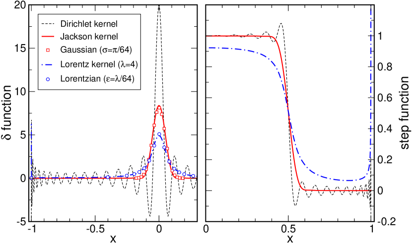
Figure 1: (Color in online edition) Order $N=64$ expansions of $\delta(x)$ (left) and a step function (right) based on different kernels. Whereas the truncated series (Dirichlet kernel) strongly oscillate, the Jackson results smoothly converge to the expanded functions. The Lorentz kernel leads to relatively poor convergence at the boundaries $x=\pm 1$, but otherwise yields perfect Lorentz-broadened approximations.

II.3.4 Lorentz kernel

The Jackson kernel derived in the preceding sections is the best choice for most of the applications we discuss below. In some situations, however, special analytical properties of the expanded functions become important, which only other kernels can account for. The Green functions that appear in the Cluster Perturbation Theory, Sec. IV.2, are an example. Considering the imaginary part of the Plemelj-Dirac formula which frequently occurs in connexion with Green functions,

$$\lim_{\epsilon\to 0}\frac{1}{x+\operatorname{i}\epsilon}=\operatorname{\mathcal{P}}\Big{(}\frac{1}{x}\Big{)}-\operatorname{i}\pi\delta(x)\,,$$ (77)

the $\delta$-function on the right hand side is approached in terms of a Lorentz curve,

$$\delta(x)=-\frac{1}{\pi}\lim_{\epsilon\to 0}\operatorname{Im}\frac{1}{x+\operatorname{i}\epsilon}=\lim_{\epsilon\to 0}\frac{\epsilon}{\pi(x^{2}+\epsilon^{2})}\,,$$ (78)

which has a different and broader shape compared to the approximations of $\delta(x)$ we get with the Jackson kernel. There are attempts to approximate Lorentzian like behavior in the framework of filter diagonalization Vijay et al. (2004), but these solutions do not lead to a positive kernel. Note that positivity of the kernel is essential to guarantee basic properties of Green functions, e.g. that poles are located in the lower (upper) half complex plane for a retarded (advanced) Green function. Since we know that the Fourier transform of a Lorentz peak is given by $\exp(-\epsilon|k|)$, we can try to construct an appropriate positive kernel assuming $a_{\nu}=\operatorname{e}^{-\lambda\nu/N}$ in Eq. (57), and indeed, after normalization, $g_{0}=1$, this yields what we call the Lorentz kernel $K_{N}^{L}(x,y)$ hereafter,

$$g_{n}^{L}=\frac{\sinh[\lambda(1-n/N)]}{\sinh(\lambda)}\,.$$ (79)

The variable $\lambda$ is a free parameter of the kernel which as a compromise between good resolution and sufficient damping of the Gibbs oscillations we empirically choose to be of the order of $3\ldots 5$. It is related to the $\epsilon$-parameter of the Lorentz curve, i.e. to its resolution, via $\epsilon=\lambda/N$. Note also, that in the limit $\lambda\to 0$ we recover the Fejér kernel $K_{N}^{F}(x,y)$ with $g_{n}^{F}=1-n/N$, suggesting that both kernels share many of their properties.

Name	$g_{n}$	Parameters	positive?	Remarks
Jackson	$\frac{1}{N+1}[(N-n+1)\cos\frac{\pi n}{N+1}+\sin\frac{\pi n}{N+1}\cot\frac{\pi}{N+1}]$	none	yes	best for most applications
Lorentz	$\sinh[\lambda(1-n/N)]/\sinh(\lambda)$	$\lambda\in\mathbb{R}$	yes	best for Green functions
Fejér	$1-n/N$	none	yes	mainly of academic interest
Lanczos	$\left(\frac{\sin(\pi n/N)}{\pi n/N}\right)^{M}$	$M\in\mathbb{N}$	no	$M=3$ closely matches the Jackson kernel, but not strictly positive Lanczos (1966)
Wang and Zunger	$\exp[-(\alpha\tfrac{n}{N})^{\beta}]$	$\alpha,\beta\in\mathbb{R}$	no	found empirically, not optimal Wang and Zunger (1994); Wang (1994)
Dirichlet	$1$	none	no	least favorable choice

Table 1: Summary of different integral kernels that can be used to improve the quality of an order $N$ Chebyshev series. The coefficients $g_{n}$ refer to Eq. (47) or (48), respectively.

In Figure 1 we compare truncated Chebyshev expansions — equivalent to using the Dirichlet kernel — to the approximations obtained with the Jackson and Lorentz kernels, which we will later use almost exclusively. Clearly, both kernels yield much better approximations to the expanded functions and, in particular, the oscillations have disappeared almost completely. The comparison with a Gaussian or Lorentzian, respectively, illustrates the nature of the broadening of a $\delta$-function under convolution with the kernels, which later on will facilitate the interpretation of our numerical results. With Table 1 we conclude this section on kernels, and, for the sake of completeness, also list two other kernels that are occasionally used in the literature. Both have certain disadvantages, in particular, they are not strictly positive.

II.4 Implementational details and remarks

II.4.1 Discrete cosine & Fourier transforms

Having discussed the theory behind Chebyshev expansion, the calculation of moments, and the various kernel approximations, let us now come to the practical issues of the implementation of KPM, namely to the reconstruction of the expanded function $f(x)$ from its moments $\mu_{n}$. Knowing a finite number $N$ of coefficients $\mu_{n}$ (see Sec. III for examples and details), we usually want to reconstruct $f(x)$ on a finite set of abscissas $x_{k}$. Naively we could sum up Eq. (47) separately for each point, thereby making use of the recursion relations for $T_{n}$, i.e.,

$$f(x_{k})=\frac{1}{\pi\sqrt{1-x_{k}^{2}}}\left[g_{0}\mu_{0}+2\sum_{n=1}^{N-1}g_{n}\mu_{n}\,T_{n}(x_{k})\right].$$ (80)

For a set $\{x_{k}\}$ containing $\tilde{N}$ points these summations would require of the order of $N\tilde{N}$ operations. We can do much better, however, remembering the definition of the Chebyshev polynomials $T_{n}$, Eq. (8), and the close relation between KPM and Fourier expansion: First, we may introduce the short-hand notation

$$\tilde{\mu}_{n}=\mu_{n}g_{n}$$ (81)

for the kernel improved moments. Second and more important, we make a special choice for our data points,

$$x_{k}=\cos\frac{\pi(k+1/2)}{\tilde{N}}\quad\text{with}\quad k=0,\ldots,(\tilde{N}-1)\,,$$ (82)

which coincides with the abscissas of Chebyshev numerical integration Abramowitz and Stegun (1970). The number $\tilde{N}$ of points in the set $\{x_{k}\}$ is not necessarily the same as the number of moments $N$. Usually we will consider $\tilde{N}\geq N$ and a reasonable choice is, e.g. $\tilde{N}=2N$. All values $f(x_{k})$ can now be obtained through a discrete cosine transform,

$$\begin{split}\gamma_{k}&=\pi\sqrt{1-x_{k}^{2}}\ f(x_{k})\\ &=\tilde{\mu}_{0}+2\sum_{n=1}^{N-1}\tilde{\mu}_{n}\cos\Big{(}\frac{\pi n(k+1/2)}{\tilde{N}}\Big{)}\end{split}$$ (83)

which allows for the use of divide-and-conquer type algorithms that require only $\tilde{N}\log\tilde{N}$ operations — a clear advantage over the above estimate $N\tilde{N}$.

Routines for fast discrete cosine transform are implemented in many mathematical libraries or Fast Fourier Transform (FFT) packages, for instance, in FFTW Frigo and Johnson (2005a, b) that ships with most Linux distributions. If no direct implementation is at hand we may also use fast discrete Fourier transform. With

$$\lambda_{n}=\begin{cases}(2-\delta_{n,0})\,\tilde{\mu}_{n}\,\exp\left(\frac{\operatorname{i}\pi n}{2\tilde{N}}\right)&0<n<N\\ 0&\text{otherwise}\end{cases}$$ (84)

and the standard definition of discrete Fourier transform,

$$\tilde{\lambda}_{k}=\sum_{n=0}^{\tilde{N}-1}\lambda_{n}\exp\left(\frac{2\pi\operatorname{i}nk}{\tilde{N}}\right)\,,$$ (85)

after some reordering we find for an even number of data points

$$\gamma_{2j} =\operatorname{Re}(\tilde{\lambda}_{j})\,,$$ (86)

$$\gamma_{2j+1} =\operatorname{Re}(\tilde{\lambda}_{\tilde{N}-1-j})\,,$$ (87)

with $j=0,\ldots,\tilde{N}/2-1$. If we need only a discrete cosine transform this setup is not optimal, as it makes no use of the imaginary part which the complex FFT calculates. It turns out, however, that the “wasted” imaginary part is exactly what we need when we later calculate Green functions and other complex quantities, i.e., we can use the setup

$$\gamma_{2j} =\tilde{\lambda}_{j}\,,$$ (88)

$$\gamma_{2j+1} =\tilde{\lambda}_{\tilde{N}-1-j}^{*}\,,$$ (89)

to evaluate Eq. (140).

II.4.2 Integrals involving expanded functions

We have already mentioned that our particular choice of $x_{k}$ corresponds to the abscissas of numerical Chebyshev integration. Hence, Gauss-type numerical approximations Press et al. (1986) to integrals of the form $\int_{-1}^{1}f(x)g(x)dx$ become simple sums,

$$\int\limits_{-1}^{1}f(x)g(x)\,dx=\int\limits_{-1}^{1}\frac{\sqrt{1-x^{2}}f(x)g(x)}{\sqrt{1-x^{2}}}\,dx\\ \simeq\frac{\pi}{\tilde{N}}\sum_{k=0}^{\tilde{N}-1}\sqrt{1-x_{k}^{2}}\ f(x_{k})g(x_{k})=\frac{1}{\tilde{N}}\sum_{k=0}^{\tilde{N}-1}\gamma_{k}g(x_{k})\,,$$ (90)

where $\gamma_{k}$ denotes the raw output of the cosine or Fourier transforms defined in Eq. (83). We can use this feature, for instance, to calculate partition functions, where $f(x)$ corresponds to the expansion of the spectral density $\rho(E)$ and $g(x)$ to the Boltzmann or Fermi weight.

II.5 Generalization to higher dimension

II.5.1 Expansion of multivariate functions

For the calculation of finite-temperature dynamical correlation functions we will later need expansions of functions of two variables. Let us therefore comment on the generalization of the previous considerations to $d$-dimensional space, which is easily obtained by extending the scalar product $\langle.|.\rangle_{2}$ to functions $f,g:[-1,1]^{d}\rightarrow\mathbb{R}$,

$$\langle f|g\rangle_{2}=\int\limits_{-1}^{1}\cdots\int\limits_{-1}^{1}f(\vec{x})g(\vec{x})\Big{(}\prod_{j=1}^{d}\pi\sqrt{1-x_{j}^{2}}\Big{)}\,dx_{1}\ldots dx_{d}\,.$$ (91)

Here $x_{j}$ denote the $d$ components of the vector $\vec{x}$. Naturally, this scalar product leads to the expansion

$$f(\vec{x}) =\sum_{\vec{n}=\vec{0}}^{\infty}\frac{\langle f|\phi_{\vec{n}}\rangle_{2}}{\langle\phi_{\vec{n}}|\phi_{\vec{n}}\rangle_{2}}\ \phi_{\vec{n}}(\vec{x})$$ (92)

$$=\frac{\sum_{\vec{n}=\vec{0}}^{\infty}\mu_{\vec{n}}h_{\vec{n}}\ \prod_{j=1}^{d}T_{n_{j}}(x_{j})}{\prod_{j=1}^{d}\pi\sqrt{1-x_{j}^{2}}}\,,$$

where we introduced a vector notation for indices, $\vec{n}=\{n_{1},\ldots,n_{d}\}$, and the following functions and coefficients

$$\phi_{\vec{n}}(\vec{x}) =\prod_{j=1}^{d}\phi_{n_{j}}(x_{j})\,,$$ (93)

$$\mu_{\vec{n}} =\langle f|\phi_{\vec{n}}\rangle_{2}{}$$

$$=\int\limits_{-1}^{1}\cdots\int\limits_{-1}^{1}f(\vec{x})\Big{(}\prod_{j=1}^{d}T_{n_{j}}(x_{j})\Big{)}\,dx_{1}\ldots dx_{d}\,,$$ (94)

$$h_{\vec{n}} =\frac{1}{\langle\phi_{\vec{n}}|\phi_{\vec{n}}\rangle_{2}}=\prod_{j=1}^{d}\frac{2}{1+\delta_{n_{j},0}}\,.$$ (95)

II.5.2 Kernels for multidimensional expansions

As in the one-dimensional case, a simple truncation of the infinite series will lead to Gibbs oscillations and poor convergence. Fortunately, we can easily generalize our previous results for kernel approximations. In particular, we find that the extended kernel

$$K_{N}(\vec{x},\vec{y})=\prod_{j=1}^{d}K_{N}(x_{j},y_{j})$$ (96)

maps an infinite series onto an truncated series,

$$f_{\text{KPM}}(\vec{x}) =\langle K_{N}(\vec{x},\vec{y})|f(\vec{y})\rangle_{2}$$ (97)

$$=\frac{\sum_{\vec{n}=\vec{0}}^{N-1}\mu_{\vec{n}}h_{\vec{n}}\ \prod_{j=1}^{d}g_{n_{j}}T_{n_{j}}(x_{j})}{\prod_{j=1}^{d}\pi\sqrt{1-x_{j}^{2}}}\,,$$

where we can take the $g_{n}$ of any of the previously discussed kernels. If we use the $g_{n}^{J}$ of the Jackson kernel, $K_{N}^{J}(\vec{x},\vec{y})$ fulfils generalizations of our conditions for an optimal kernel, namely

1. $K_{N}^{J}(\vec{x},\vec{y})$ is positive $\forall\ \vec{x},\vec{y}\in[-1,1]^{d}$.

2. $K_{N}^{J}(\vec{x},\vec{y})$ is normalized with

   $$\int\limits_{-1}^{1}\cdots\int\limits_{-1}^{1}f_{\text{KPM}}(\vec{x})\,dx_{1}\ldots dx_{d}=\int\limits_{-1}^{1}\cdots\int\limits_{-1}^{1}f(\vec{x})\,dx_{1}\ldots dx_{d}\,.$$ (98)

3. $K_{N}^{J}(\vec{x},\vec{y})$ has optimal resolution in the sense that

   $$Q =\int\limits_{-1}^{1}\cdots\int\limits_{-1}^{1}(\vec{x}-\vec{y})^{2}K_{N}(\vec{x},\vec{y})\,dx_{1}\ldots dx_{d}\,dy_{1}\ldots dy_{d}$$ (99)

   $$=d(g_{0}-g_{1})$$

   is minimal.

Note that for simplicity the order of the expansion, $N$, was chosen to be the same for all spatial directions. Of course, we could also define more general kernels,

$$K_{\vec{N}}(\vec{x},\vec{y})=\prod_{j=1}^{d}K_{N_{j}}(x_{j},y_{j})\,,$$ (100)

where the vector $\vec{N}$ denotes the orders of expansion for the different spatial directions.

II.5.3 Reconstruction with cosine transforms

Similar to the 1D case we may consider the function $f:[-1,1]^{d}\rightarrow\mathbb{R}$ on a discrete grid $\vec{x}_{\vec{k}}$ with

$$x_{\vec{k},j} =\cos(\varphi_{k_{j}})\,,$$ (101)

$$\varphi_{k_{j}} =\frac{\pi(k_{j}+1/2)}{\tilde{N}}\,,$$ (102)

$$k_{j} =0,\ldots,(\tilde{N}-1)\,.$$ (103)

Note again that we could define individual numbers of points for each spatial direction, i.e., a vector $\vec{\tilde{N}}$ with elements $\tilde{N}_{j}$ instead of a single $\tilde{N}$. For all grid points $\vec{x}_{\vec{k}}$ the function $f(\vec{x}_{\vec{k}})$ is obtained through multidimensional discrete cosine transform, i.e., with coefficients $\kappa_{\vec{n}}=\tilde{\mu}_{\vec{n}}h_{\vec{n}}=\mu_{\vec{n}}g_{\vec{n}}h_{\vec{n}}$ we find

$$\gamma_{\vec{k}} =f({\cos(\varphi_{k_{1}}),\ldots,\cos(\varphi_{k_{d}})})\prod_{j=1}^{d}\pi\sin(\varphi_{k_{j}})$$ (104)

$$=\sum_{\vec{n}=\vec{0}}^{N-1}\kappa_{\vec{n}}\prod_{j=1}^{d}\cos(n_{j}\varphi_{k_{j}})$$

$$=\sum_{n_{1}=0}^{N-1}\cos(n_{1}\varphi_{k_{1}})\ldots\sum_{n_{d}=0}^{N-1}\cos(n_{d}\varphi_{k_{d}})\kappa_{\vec{n}}\,.$$

The last line shows that the multidimensional discrete cosine transform is equivalent to a nesting of one-dimensional transforms in every coordinate. With fast implementations the computational effort is thus proportional to $d\tilde{N}^{d-1}\tilde{N}\log\tilde{N}$, which equals the expected value for $\tilde{N}^{d}$ data points, $\tilde{N}^{d}\log\tilde{N}^{d}$. If we are not using libraries like FFTW, which provide ready-to-use multidimensional routines, we may also resort to one-dimensional cosine transform or the above translation into FFT to obtain high-performance implementations of general $d$-dimensional transforms.

III Applications of KPM

Having described the mathematical background and many details of the implementation of the Kernel Polynomial Method, we are now in the position to present practical applications of the approach. Already in the introduction we have mentioned that KPM can be used whenever we are interested in the spectral properties of large matrices or in correlation functions that can be expressed through the eigenstates of such matrices. Apparently, this leads to a vast range of applications. In what follows, we try to cover all types of accessible quantities and for each give at least one example. We thereby focus on lattice models from solid state physics.

III.1 Densities of states

III.1.1 General considerations

The first and basic application of Chebyshev expansion and KPM is the calculation of the spectral density of Hermitian matrices, which could correspond to the densities of states of both interacting or non-interacting quantum models Wheeler (1974); Skilling (1988); Silver and Röder (1994); Silver et al. (1996). To be specific, let us consider a $D$-dimensional matrix $M$ with eigenvalues $E_{k}$, whose spectral density is defined as

$$\rho(E)=\frac{1}{D}\sum_{k=0}^{D-1}\delta(E-E_{k})\,.$$ (105)

As described earlier, the expansion of $\rho(E)$ in terms of Chebyshev polynomials requires a rescaling of $M\rightarrow\tilde{M}$, such that the spectrum of $\tilde{M}=(M-b)/a$ lies within the interval $[-1,1]$. Given the eigenvalues $\tilde{E}_{k}$ of $\tilde{M}$ the rescaled density $\tilde{\rho}(\tilde{E})$ reads

$$\tilde{\rho}(\tilde{E})=\frac{1}{D}\sum_{k=0}^{D-1}\delta(\tilde{E}-\tilde{E}_{k})\,,$$ (106)

and according to Eq. (19) the expansion coefficients become

$$\mu_{n} =\int\limits_{-1}^{1}\tilde{\rho}(\tilde{E})\,T_{n}(\tilde{E})\,d\tilde{E}=\frac{1}{D}\sum_{k=0}^{D-1}T_{n}(\tilde{E}_{k})$$ (107)

$$=\frac{1}{D}\sum_{k=0}^{D-1}\langle k|T_{n}(\tilde{M})|k\rangle=\frac{1}{D}\,\operatorname{Tr}(T_{n}(\tilde{M}))\,.$$

This is exactly the trace form that we introduced in Sec. II.2, and we can immediately calculate the $\mu_{n}$ using the stochastic techniques described in Sec. II.2.2. Knowing the moments we can use the techniques of Sec. II.4 to reconstruct $\tilde{\rho}(\tilde{E})$ for the whole range $[-1,1]$, and a final rescaling yields $\rho(E)$.

III.1.2 Non-interacting systems: Anderson model of disorder

Applied to a generalized model of non-interacting fermions $c_{i}^{(\dagger)}$,

$$H=\sum_{i,j=0}^{D-1}c_{i}^{\dagger}M_{ij}c_{j}\,,$$ (108)

the matrix of interest $M$ is formed by the coupling constants $M_{ij}$. Knowing the spectrum of $M$, i.e. the single-particle density of states $\rho(E)$, all thermodynamic quantities of the model can be calculated. For example, the particle density is given by

$$n=\int\frac{\rho(E)}{1+\operatorname{e}^{\beta(E-\mu)}}\,dE$$ (109)

and the free energy per site reads

$$f=n\mu-\frac{1}{\beta}\int\rho(E)\,\log(1+\operatorname{e}^{-\beta(E-\mu)})\,dE\,,$$ (110)

where $\mu$ is the chemical potential and $\beta=1/T$ the inverse temperature.

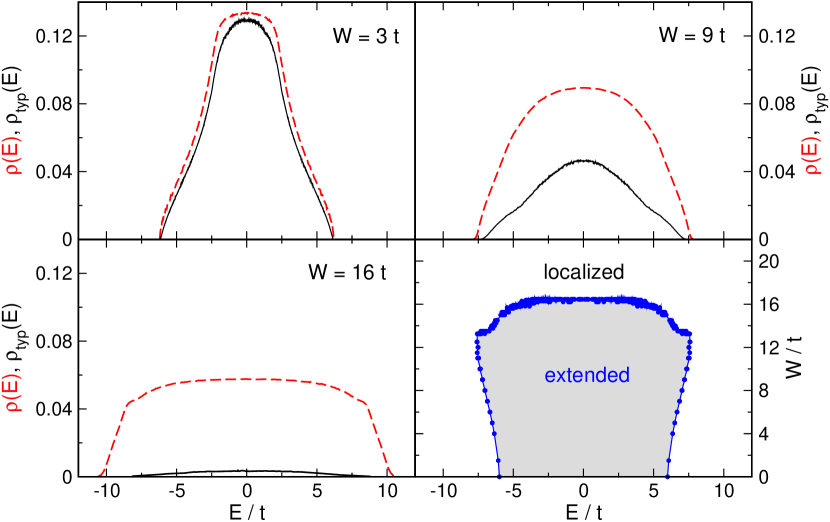
Figure 2: (Color in online edition) Standard (dashed) and typical density of states (solid line), $\rho(E)$ and $\rho_{\text{typ}}(E)$ respectively, of the 3D Anderson model on a $50^{3}$ site cluster with periodic boundary conditions. For $\rho(E)$ we calculated $N=2048$ moments with $R=10$ start vectors and $S=240$ realizations of disorder, for $\rho_{\text{typ}}(E)$ these numbers are $N=8192$, $R=32$ and $S=200$. The lower right panel shows the phase diagram of the model we obtained from $\rho_{\text{typ}}(E)/\rho(E)\to 0$ (mobility edge).

As the first physical example let us consider the Anderson model of non-interacting fermions moving in a random potential Anderson (1958),

$$H=-t\sum_{\langle ij\rangle}c_{i}^{\dagger}c_{j}+\sum_{i}\epsilon_{i}c_{i}^{\dagger}c_{i}\,.$$ (111)

Here hopping occurs along nearest neighbor bonds $\langle ij\rangle$ on a simple cubic lattice and the local potential $\epsilon_{i}$ is chosen randomly with uniform distribution in the interval $[-W/2,W/2]$. With increasing strength of disorder, $W$, the single-particle eigenstates of the model tend to become localized in the vicinity of a particular lattice site, which excludes these states from contributing to electronic transport. Disorder can therefore drive a transition from metallic behavior with delocalized fermions to insulating behavior with localized fermions Thouless (1974); Lee and Ramakrishnan (1985); Kramer and Mac Kinnon (1993). The disorder averaged density of states $\rho(E)$ of the model can be obtained as described, but it contains no information about localization. The KPM method, however, allows also for the calculation of the local density of states,

$$\rho_{i}(E)=\frac{1}{D}\sum_{k=0}^{D-1}|\langle i|k\rangle|^{2}\,\delta(E-E_{k})\,,$$ (112)

which is a measure for the contribution of a single lattice site (denoted by the basis state $|i\rangle$) to the complete spectrum. For delocalized states all sites contribute equally, whereas localized states reside on just a few sites, or, equivalently, a certain site contributes only to a few eigenstates. This property has a pronounced effect on the distribution of $\rho_{i}(E)$, which at a fixed energy $E$ characterizes the variation of $\rho_{i}$ over different realizations of disorder and sites $i$. For energies that correspond to localized eigenstates the distribution is highly asymmetric and becomes singular in the thermodynamic limit, whereas in the delocalized case the distribution is regular and centered near its expectation value $\rho(E)$. Therefore a comparison of the geometric and the arithmetic average of $\rho_{i}(E)$ over a set of realizations of disorder and over lattice sites reveals the position of the Anderson transition Dobrosavljević and Kotliar (1997, 1998); Schubert et al. (2005b, a). The expansion of $\rho_{i}(E)$ is even simpler than the expansion of $\rho(E)$, since the moments have the form of expectation values and do not involve a trace,

$$\mu_{n} =\int\limits_{-1}^{1}\tilde{\rho}_{i}(E)\,T_{n}(E)\,dE=\frac{1}{D}\sum_{k=0}^{D-1}|\langle i|k\rangle|^{2}T_{n}(\tilde{E}_{k})$$ (113)

$$=\frac{1}{D}\sum_{k=0}^{D-1}\langle i|T_{n}(\tilde{M})|k\rangle\langle k|i\rangle=\frac{1}{D}\ \langle i|T_{n}(\tilde{M})|i\rangle\,.$$

In Figure 2 we show the standard density of states $\rho(E)$, which coincides with the arithmetic mean of $\rho_{i}(E)$, in comparison to the typical density of states $\rho_{\text{typ}}(E)$, which is defined as the geometric mean of $\rho_{i}(E)$,

$$\rho_{\text{typ}}(E)=\exp[\big{\langle}\!\!\big{\langle}\log(\rho_{i}(E))\big{\rangle}\!\!\big{\rangle}]\,.$$ (114)

With increasing disorder, starting from the boundaries of the spectrum, $\rho_{\text{typ}}(E)$ is suppressed until it vanishes completely for $W/t\gtrsim 16.5$, which is known as the critical strength of disorder where the states in the band center become localized Slevin and Ohtsuki (1999). The calculation yields the phase diagram shown in the lower right corner of Figure 2, which compares well to other numerical results.

Since the method requires storage only for the sparse Hamiltonian matrix and for two vectors of the corresponding dimension, quite large systems can be studied on standard desktop computers (of the order of $100^{3}$ sites). The recursion is stable for arbitrarily high expansion order. In the present case we calculated as many as $8192$ moments to achieve maximum resolution in the local density of states. The standard density of states is usually far less demanding.

III.1.3 Interacting systems: Double exchange

Coming to interacting quantum systems, as a second example we study the evolution of the quantum double-exchange model Anderson and Hasegawa (1955) for large spin amplitude $S$, which in terms of spin-less fermions $c_{i}^{(\dagger)}$ and Schwinger bosons $a_{i\sigma}^{(\dagger)}$ ($\sigma=\uparrow,\downarrow$) is given by the Hamiltonian

$$H=-\frac{t}{2S+1}\sum_{\langle ij\rangle,\sigma}a_{i\sigma}^{\dagger}a_{j\sigma}c_{i}^{\dagger}c_{j}$$ (115)

with the local constraint $\sum_{\sigma}a_{i\sigma}^{\dagger}a_{i\sigma}=2S+c_{i}^{\dagger}c_{i}$. This model describes itinerant electrons on a lattice whose spin is strongly coupled to local spins of amplitude $S$, so that the motion of the electrons mediates an effective ferromagnetic interaction between these localized spins. In the case of colossal magneto-resistant manganites Coey et al. (1999), for instance, cubic site symmetry leads to a crystal field splitting of the manganese $d$-shell, and three electrons in the resulting $t_{2g}$-shell form the local spins. The remaining electrons occupy the $e_{g}$-shell and can become itinerant upon doping, causing these materials to show ferromagnetic order Zener (1951). If the ferromagnetic (Hund’s rule) coupling is large, at each site only the high-spin states are relevant and we can describe the total on-site spin in terms of Schwinger bosons $a_{i\sigma}^{(\dagger)}$ Auerbach (1994). From the electrons only the charge degree of freedom remains, which is denoted by the spin-less fermions $c_{i}^{(\dagger)}$ (see, e.g. Weiße et al. (2001) for more details). The full quantum model, Eq. (115), is rather complicated for analytical or numerical studies, and we expect major simplification by treating the spin background classically (remember that $S$ is quite large for the systems of interest). The limit of classical spins, $S\rightarrow\infty$, is obtained by averaging Eq. (115) over spin coherent states,

$$|\Omega(S,\theta,\phi)\rangle=\frac{\big{(}\cos(\frac{\theta}{2})\operatorname{e}^{\operatorname{i}\phi/2}a_{\uparrow}^{\dagger}+\sin(\frac{\theta}{2})\operatorname{e}^{-\operatorname{i}\phi/2}a_{\downarrow}^{\dagger}\big{)}^{2S}}{\sqrt{(2S)!}}\ |0\rangle\,,$$ (116)

where $\theta$ and $\phi$ are the classical polar angles and $|0\rangle$ the bosonic vacuum. The resulting non-interacting Hamiltonian reads,

$$H=-\sum_{\langle ij\rangle}t_{ij}c_{i}^{\dagger}c_{j}+\textrm{H.c.}\,,$$ (117)

with the matrix element Kogan and Auslender (1988)

$$t_{ij}=t\big{[}\cos\tfrac{\theta_{i}}{2}\cos\tfrac{\theta_{j}}{2}\ \operatorname{e}^{-\operatorname{i}(\phi_{i}-\phi_{j})/2}\\ +\sin\tfrac{\theta_{i}}{2}\sin\tfrac{\theta_{j}}{2}\ \operatorname{e}^{\operatorname{i}(\phi_{i}-\phi_{j})/2}\big{]}\,,$$ (118)

i.e., spin-less fermions move in a background of random or ordered classical spins which affect their hopping amplitude.

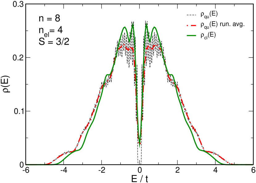
Figure 3: (Color in online edition) Density of nonzero eigenvalues of the quantum double-exchange model with $S=3/2$ (dashed line) and running average (red dot-dashed), calculated for 4 electrons on a 8-site ring, compared to the classical result $S\rightarrow\infty$ (green solid). Expansion parameters: $N=400$ moments and $R=100$ random vectors per $S^{z}$ sector.

To assess the quality of this classical approximation we considered four electrons moving on a ring of eight sites, and compared the densities of states obtained for a background of $S=3/2$ quantum spins and a background of classical spins. For the full quantum Hamiltonian, Eq. (115), the (canonical) density of states was calculated on the basis of $400$ Chebyshev moments. To reduce the Hilbert space dimension and to save resources we made use of the $SU(2)$ symmetry of the model: With the stochastic approach we calculated separate moments $\mu_{n}^{S^{z}}$ for each $S^{z}$-sector,

$$\mu_{n}^{S^{z}}=\operatorname{Tr}^{S^{z}}[T_{n}(\tilde{H})]\,,$$ (119)

and used the dimensions $D^{S^{z}}$ of the sectors to obtain the total normalized $\mu_{n}$ from the average

$$\mu_{n}=\frac{1}{D}\operatorname{Tr}[T_{n}(\tilde{H})]=\frac{\sum\limits_{S^{z}=-S^{\text{max}}}^{S^{\text{max}}}\mu_{n}^{S^{z}}}{\sum\limits_{S^{z}=-S^{\text{max}}}^{S^{\text{max}}}D^{S^{z}}}\,.$$ (120)

Note, that such a setup can be used whenever the model under consideration has certain symmetries.

On the other hand, we solved the effective non-interacting model (117) and calculated the distributions of non-zero energies for a background of fully disordered classical spins. As Figure 3 illustrates, the spectrum of the quantum model with $S=3/2$ closely matches that of the system with classical spins, providing good justification, e.g. for studies of colossal magneto-resistive manganites that make use of a classical approximation for the spin background. Since for the finite cluster considered the spectrum of the quantum model is discrete, at the present expansion order KPM starts to resolve distinct energy levels (dashed line). Therefore a running average (dot-dashed line) compares better to the classical spin-averaged data (bold line).

III.2 Static correlations at finite temperature

Densities of states provide only the most basic information about a given quantum system, and much more details can usually be learned from the study of correlations and the response of the system to an external probe or perturbation. Starting with static correlation functions, let us now extend the application range of the expansion techniques to such more involved quantities.

Given the eigenstates $|k\rangle$ of an interacting quantum system the thermodynamic expectation value of an operator $A$ reads

$$\langle A\rangle =\frac{1}{ZD}\operatorname{Tr}(A\operatorname{e}^{-\beta H})=\frac{1}{ZD}\sum_{k=0}^{D-1}\langle k|A|k\rangle\,\operatorname{e}^{-\beta E_{k}}\,,$$ (121)

$$Z =\frac{1}{D}\operatorname{Tr}(\operatorname{e}^{-\beta H})=\frac{1}{D}\sum_{k=0}^{D-1}\operatorname{e}^{-\beta E_{k}}\,,$$ (122)

where $H$ is the Hamiltonian of the system, $Z$ the partition function, and $E_{k}$ the energy of the eigenstate $|k\rangle$. Using the function

$$a(E)=\frac{1}{D}\sum_{k=0}^{D-1}\langle k|A|k\rangle\,\delta(E-E_{k})$$ (123)

and the (canonical) density of states $\rho(E)$, we can express the thermal expectation value in terms of integrals over the Boltzmann weight,

$$\langle A\rangle =\frac{1}{Z}\int\limits_{-\infty}^{\infty}a(E)\,\operatorname{e}^{-\beta E}\,dE\,,$$ (124)

$$Z =\int\limits_{-\infty}^{\infty}\rho(E)\,\operatorname{e}^{-\beta E}\,dE\,.$$ (125)

Of course, similar relations hold also for non-interacting fermion systems, where the Boltzmann weight $\operatorname{e}^{-\beta E}$ has to be replaced by the Fermi function $f(E)=(1+\operatorname{e}^{\beta(E-\mu)})^{-1}$ and the single-electron wave functions play the role of $|k\rangle$.

Again, the particular form of $a(E)$ suggests an expansion in Chebyshev polynomials, and after rescaling we find

$$\mu_{n}=\int\limits_{-1}^{1}\tilde{a}(E)\,T_{n}(E)\,dE =\frac{1}{D}\sum_{k=0}^{D-1}\langle k|A|k\rangle\,T_{n}(\tilde{E}_{k})$$ (126)

$$=\frac{1}{D}\operatorname{Tr}(AT_{n}(\tilde{H}))\,,$$

which can be evaluated with the stochastic approach, Sec. II.2.2.

Figure 4: (Color in online edition) Nearest-neighbor $S^{z}$-$S^{z}$ correlations of the XXZ model on a square lattice. Lines represent the KPM results with separation of low-lying eigenstates (bold solid and bold dashed) and without (thin dashed), open symbols denote exact results from a complete diagonalization of a $4\times 4$ system.

For interacting systems at low temperature the expression in Eq. (124) is a bit problematic, since the Boltzmann factor puts most of the weight on the lower end of the spectrum and heavily amplifies small numerical errors in $\rho(E)$ and $a(E)$. We can avoid these problems by calculating the ground state and some of the lowest excitations exactly, using standard iterative diagonalization methods like Lanczos or Jacobi-Davidson. Then we split the expectation value of $A$ and the partition function $Z$ into contributions from the exactly known states and contributions from the rest of the spectrum,

$$\langle A\rangle =\frac{1}{ZD}\sum_{k=0}^{C-1}\langle k|A|k\rangle\,\operatorname{e}^{-\beta E_{k}}+\frac{1}{Z}\int\limits_{-\infty}^{\infty}a_{s}(E)\operatorname{e}^{-\beta E}\,dE\,,$$ (127)

$$Z =\frac{1}{D}\sum_{k=0}^{C-1}\operatorname{e}^{-\beta E_{k}}+\int\limits_{-\infty}^{\infty}\rho_{s}(E)\operatorname{e}^{-\beta E}\,dE$$ (128)

The functions

$$a_{s}(E) =\frac{1}{D}\sum_{k=C}^{D-1}\langle k|A|k\rangle\,\delta(E-E_{k})\,,$$ (129)

$$\rho_{s}(E) =\frac{1}{D}\sum_{k=C}^{D-1}\delta(E-E_{k})$$ (130)

describe the rest of the spectrum and can be expanded in Chebyshev polynomials easily. Based on the known states we can introduce the projection operator

$$P=1-\sum_{k=0}^{C-1}|k\rangle\langle k|\,,$$ (131)

and find for the expansion coefficients of $\tilde{a}_{s}(E)$

$$\mu_{n}=\frac{1}{D}\operatorname{Tr}(PAT_{n}(\tilde{H}))\approx\frac{1}{RD}\sum_{r=0}^{R-1}\langle r|PAT_{n}(\tilde{H})P|r\rangle\,,$$ (132)

and similarly for those of $\tilde{\rho}_{s}(E)$

$$\mu_{n}=\frac{1}{D}\operatorname{Tr}(PT_{n}(\tilde{H}))\approx\frac{1}{RD}\sum_{r=0}^{R-1}\langle r|PT_{n}(\tilde{H})P|r\rangle\,.$$ (133)

Note, that in addition to the two vectors for the Chebyshev recursion we now need memory also for the eigenstates $|k\rangle$. Otherwise the resource consumption is the same as in the standard scheme.

We illustrate the accuracy of this approach in Figure 4 considering the nearest-neighbor $S^{z}$-$S^{z}$ correlations of the square-lattice spin-$1/2$ XXZ model as an example,

$$H=\sum_{i,\delta}(S_{i}^{x}S_{i+\delta}^{x}+S_{i}^{y}S_{i+\delta}^{y}+\Delta S_{i}^{z}S_{i+\delta}^{z})\,.$$ (134)

As a function of temperature and for an anisotropy $-1<\Delta<0$ this model shows a quantum to classical crossover in the sense that the correlations are anti-ferromagnetic at low temperature (quantum effect) and ferromagnetic at high temperature (as expected for the classical model). Fabricius and McCoy (1999); Schindelin et al. (2000); Fehske et al. (2000) Comparing the KPM results with the exact correlations of a $4\times 4$ system, which were obtained from a complete diagonalization of the Hamiltonian, the improvement due to the separation of only a few low-lying eigenstates is obvious. Whereas for $C=0$ the data is more or less random below $T\approx 1$, the agreement with the exact data is perfect, if the ground state and one or two excitations are considered separately. The numerical effort required for these calculations differs largely between complete diagonalization and the KPM method. For the former, $18$ or $20$ sites are practically the limit, whereas the latter can easily handle $30$ sites or more.

Note that for non-interacting systems the above separation of the spectrum is not required, since for $T\to 0$ the Fermi function converges to a simple step function without causing any numerical problems.

III.3 Dynamical correlations at zero temperature

III.3.1 General considerations

Having discussed simple expectation values and static correlations, the calculation of time dependent quantities is the natural next step in the study of complex quantum models. This is motivated also by many experimental setups, which probe the response of a physical system to time dependent external perturbations. Examples are inelastic scattering experiments or measurements of transport coefficients. In the framework of linear response theory and the Kubo formalism the system’s response is expressed in terms of dynamical correlation functions, which can also be calculated efficiently with Chebyshev expansion and KPM. Technically though, we need to distinguish between two different situations: For interacting many-particle systems at zero temperature only matrix elements between the ground state and excited states contribute to a dynamical correlation function, whereas for interacting systems at finite temperature or for non-interacting systems with a finite particle density transitions between all eigenstates — many-particle or single-particle, respectively — contribute. We therefore split the discussion of dynamical correlations into two sections, starting here with interacting many-particle systems at $T=0$.

Given two operators $A$ and $B$ a general dynamical correlation function can be defined through

$$\langle A;B\rangle_{\omega}^{\pm}=\lim_{\epsilon\to 0}\ \langle 0|A\frac{1}{\omega+\operatorname{i}\epsilon\mp H}B|0\rangle\\ =\lim_{\epsilon\to 0}\sum\limits_{k=0}^{D-1}\frac{\langle 0|A|k\rangle\langle k|B|0\rangle}{\omega+\operatorname{i}\epsilon\mp E_{k}}\,,$$ (135)

where $E_{k}$ is the energy of the many-particle eigenstate $|k\rangle$ of the Hamiltonian $H$, $|0\rangle$ its ground state, and $\epsilon>0$.

If we assume that the product $\langle 0|A|k\rangle\langle k|B|0\rangle$ is real the imaginary part

$$\operatorname{Im}\langle A;B\rangle_{\omega}^{\pm}=-\pi\sum\limits_{k=0}^{D-1}\langle 0|A|k\rangle\langle k|B|0\rangle\,\delta(\omega\mp E_{k})$$ (136)

has a similar structure as, e.g., the local density of states in Eq. (112), and in fact, with $\rho_{i}(E)$ we already calculated a dynamical correlation function. Hence, after rescaling the Hamiltonian $H\to\tilde{H}$ and all energies $\omega\to\tilde{\omega}$ we can proceed as usual and expand $\operatorname{Im}\langle A;B\rangle_{\omega}^{\pm}$ in Chebyshev polynomials,

$$\operatorname{Im}\langle A;B\rangle_{\tilde{\omega}}^{\pm}=-\frac{1}{\sqrt{1-\tilde{\omega}^{2}}}\Big{[}\mu_{0}+2\sum\limits_{n=1}^{\infty}\mu_{n}\,T_{n}(\tilde{\omega})\Big{]}\,.$$ (137)

Again, the moments are obtained from expectation values

$$\mu_{n}=\frac{1}{\pi}\int\limits_{-1}^{1}\operatorname{Im}\langle A;B\rangle_{\tilde{\omega}}^{\pm}\,T_{n}(\tilde{\omega})\,d\tilde{\omega}=\langle 0|AT_{n}(\mp\tilde{H})B|0\rangle\,,$$ (138)

and for $A\neq B^{\dagger}$ we can follow the scheme outlined in Eqs. (30) to (33). For $A=B^{\dagger}$ the calculation simplifies to the one in Eqs. (34) and (35), now with $B|0\rangle$ as the starting vector.

In many cases, especially for the spectral functions and optical conductivities studied below, only the imaginary part of $\langle A;B\rangle_{\omega}^{\pm}$ is of interest, and the above setup is all we need. Sometimes however — e.g., within the Cluster Perturbation Theory discussed in Sec. IV.2 — also the real part of a general correlation function $\langle A;B\rangle_{\omega}^{\pm}$ is required. Fortunately it can be calculated with almost no additional effort: The analytical properties of $\langle A;B\rangle_{\omega}^{\pm}$ arising from causality imply that its real part is fully determined by the imaginary part. Indeed a Hilbert transform gives

$$\operatorname{Re}\langle A;B\rangle_{\tilde{\omega}}^{\pm}=\sum\limits_{k=0}^{D-1}\langle 0|A|k\rangle\langle k|B|0\rangle\,\operatorname{\mathcal{P}}\left(\frac{1}{\tilde{\omega}\mp\tilde{E}_{k}}\right)\\ =-\frac{1}{\pi}\operatorname{\mathcal{P}}\int\limits_{-1}^{1}\frac{\operatorname{Im}\langle A;B\rangle_{\tilde{\omega}^{\prime}}^{\pm}}{\tilde{\omega}-\tilde{\omega}^{\prime}}\,d\omega^{\prime}=-2\sum\limits_{n=1}^{\infty}\mu_{n}\,U_{n-1}(\tilde{\omega})\,,$$ (139)

where we used Eq. (14). The full correlation function

$$\langle A;B\rangle_{\tilde{\omega}}^{\pm} =\frac{-\operatorname{i}\mu_{0}}{\sqrt{1-\tilde{\omega}^{2}}}-2\sum\limits_{n=1}^{\infty}\mu_{n}\Big{[}U_{n-1}(\tilde{\omega})+\frac{\operatorname{i}\,T_{n}(\tilde{\omega})}{\sqrt{1-\tilde{\omega}^{2}}}\Big{]}$$ (140)

$$=\frac{-\operatorname{i}}{\sqrt{1-\tilde{\omega}^{2}}}\Big{[}\mu_{0}+2\sum\limits_{n=1}^{\infty}\mu_{n}\exp(-\operatorname{i}n\arccos\tilde{\omega})\Big{]}$$

can thus be reconstructed from the same moments $\mu_{n}$ that we derived for its imaginary part, Eq. (138). In contrast to the real quantities we considered so far, the reconstruction merely requires complex Fourier transform, see Eqs. (88) and (89). If only the imaginary or real part of $\langle A;B\rangle_{\omega}^{\pm}$ is needed, a cosine or sine transform, respectively, is sufficient.

Note again, that the calculation of dynamical correlation functions for non-interacting electron systems is not possible with the scheme discussed in this section, not even at zero temperature. At finite band filling (finite chemical potential) the ground state consists of a sum over occupied single-electron states, and dynamical correlation functions thus involve a double summation over matrix elements between all single-particle eigenstates, weighted by the Fermi function. Clearly, this is more complicated than Eq. (135), and we postpone the discussion of this case to Sec. III.4, where we describe methods for dynamical correlation functions at finite temperature and — for the case of non-interacting electrons — finite density.

III.3.2 One-particle spectral function

An important example of a dynamical correlation function is the (retarded) Green function in momentum space,

$$G_{\sigma}(\vec{k},\omega)=\langle c^{\phantom{\dagger}}_{\vec{k},\sigma};c^{\dagger}_{\vec{k},\sigma}\rangle_{\omega}^{+}+\langle c^{\dagger}_{\vec{k},\sigma};c^{\phantom{\dagger}}_{\vec{k},\sigma}\rangle_{\omega}^{-}\,,$$ (141)

and the associated spectral function

$$\begin{split}A_{\sigma}(\vec{k},\omega)&=-\frac{1}{\pi}\operatorname{Im}\,G_{\sigma}(\vec{k},\omega)\\ &=A^{+}_{\sigma}(\vec{k},\omega)+A^{-}_{\sigma}(\vec{k},\omega)\,,\end{split}$$ (142)

which characterizes the electron absorption or emission of an interacting system. For instance, $A^{-}_{\sigma}$ can be measured experimentally in angle resolved photo-emission spectroscopy (ARPES).

As the first application, let us consider the one-dimensional Holstein model for spinless fermions Holstein (1959a, b),

$$H=-t\sum_{i}(c_{i}^{\dagger}c_{i+1}+\text{H.c.})\\ -g\omega_{0}\sum_{i,\sigma}(b_{i}^{\dagger}+b_{i})n_{i}+\omega_{0}\sum_{i}b_{i}^{\dagger}b_{i}\,,$$ (143)

which is one of the basic models for the study of electron-lattice interaction. A single band of electrons is approximated by spinless fermions $c_{i}^{(\dagger)}$, the density of which couples to the local lattice distortion described by dispersionless phonons $b_{i}^{(\dagger)}$. At low fermion density, with increasing electron phonon interaction the charges get dressed by a surrounding lattice distortion and form new, heavy quasi-particles known as polarons. Eventually, for strong coupling the width of the corresponding band is suppressed exponentially, leading to a process called self-trapping. For a half-filled band, i.e., $0.5$ fermions per site, the model allows for the study of quantum effects at the transition from a metal to a band (or Peierls) insulator, marked by the opening of a gap at the Fermi wave vector and the development of a matching lattice distortion.

Since the Hamiltonian (143) involves bosonic degrees of freedom, the Hilbert space of even a finite system has infinite dimension. In practice, nevertheless, the contribution of highly excited phonon states is found to be negligible at low temperature or for the ground-state, and the system is well approximated by a truncated phonon space with $\sum_{i}b_{i}^{\dagger}b_{i}\leq M$ Bäuml et al. (1998). In addition, the translational symmetry of the model can be used to reduce the Hilbert space dimension, and, moreover, the symmetric phonon mode with momentum $q=0$ can be excluded from the numerics: Since it couples to the total number of electrons, which is a conserved quantity, its contribution can be handled analytically Robin (1997); Sykora et al. (2005). Below we present results for a cluster size of $L=8$ or $10$, where a cut-off $M=24$ or $15$, respectively, leads to truncation errors $<10^{-6}$ for the ground-state energy. Alternatively, for one or two fermionic particles and low temperatures an optimized variational basis can be constructed for infinite systems Bonča et al. (1999), which would also be suitable for our numerical approach.

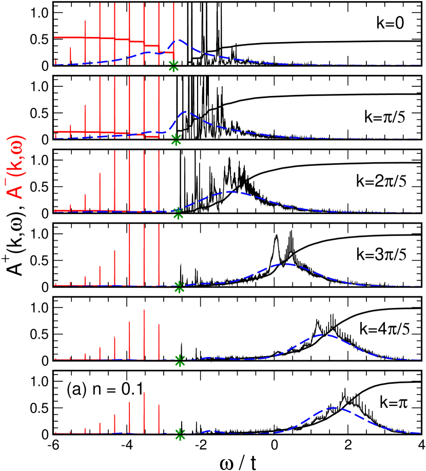
Figure 5: (Color in online edition) One-particle spectral function and its integral for the Holstein model (a) on a 10-site ring with one electron, $\varepsilon_{p}=g^{2}\omega_{0}=2.0t$, $\omega_{0}=0.4t$, and (b) on a 8-site ring, band filling $n=0.5$, $\varepsilon_{p}=g^{2}\omega_{0}=1.6t$, $\omega_{0}=0.1t$. For comparison, in (a) the blue dashed lines represent Quantum Monte Carlo data at $\beta t=8$ Hohenadler et al. (2005), and green stars indicate the position of the polaron band in the infinite system Bonča et al. (1999). In (b) the blue and green curves denote results of Dynamical DMRG for the same lattice size and $T=0$ Jeckelmann and Fehske (2006).

In Figure 5 we present KPM data for the spectral function of the spinless-fermion Holstein model and assess its quality by comparing with results from Quantum Monte Carlo (QMC) and Dynamical Density Matrix Renormalization Group (DDMRG) Jeckelmann (2002) calculations. Starting with the case of a single electron on a ten-site ring, Figure 5 (a) illustrates the presence of a narrow polaron band at the Fermi level and of a broad range of incoherent contributions to the spectral function, which in the spinless case reads

$$A^{-}(k,\omega)=\sum_{l}|\langle l,N_{\text{e}}-1|\,c_{k}\,|0,N_{\text{e}}\rangle|^{2}\\ \times\delta[\omega+(E_{l,N_{\text{e}}-1}-E_{0,N_{\text{e}}})]$$ (144)

and

$$A^{+}(k,\omega)=\sum_{l}|\langle l,N_{\text{e}}+1|\,c_{k}^{\dagger}\,|0,N_{\text{e}}\rangle|^{2}\\ \times\delta[\omega-(E_{l,N_{\text{e}}+1}-E_{0,N_{\text{e}}})]\,.$$ (145)

Here $|l,N_{\text{e}}\rangle$ denotes the $l$th eigenstate with $N_{\text{e}}$ electrons and energy $E_{l,N_{\text{e}}}$. The photo-emission part $A^{-}$ reflects the Poisson-like phonon distribution of the polaron ground state, whereas $A^{+}$ has most of its weight in the vicinity of the original free electron band. In terms of the overall shape and the integrated weight, both KPM and QMC agree very well. QMC, however, is not able to resolve all the narrow features of the spectral function, and the polaron band is hardly observable. Nevertheless, QMC has the advantage that larger systems can be studied, in particular at finite temperature. As a guide to the eye we also show the position of the polaron band in the infinite system, which was calculated with the approach of Bonča et al. (1999). In Figure 5 (b) we consider the case of a half-filled band and strong electron-phonon coupling, where the system is in an insulating phase with an excitation gap at the Fermi momentum $k=\pm\pi/2$. Below and above the gap the spectrum is characterized by broad multi-phonon absorption. Compared to DDMRG, again KPM offers the better resolution and unfolds all the discrete phonon sidebands. Concerning numerical performance DDMRG has the advantage of a small optimized Hilbert space, which can be handled with standard workstations. However, the basis optimization is rather time consuming and, in addition, each frequency value $\omega$ requires a new simulation. The KPM calculations, on the other hand, involved matrix dimensions between $10^{8}$ and $10^{10}$, and we therefore used high-performance computers such as Hitachi SR8000-F1 or IBM p690 for the moment calculation. For the reconstruction of the spectra, of course, a desktop computer is sufficient.

III.3.3 Optical conductivity

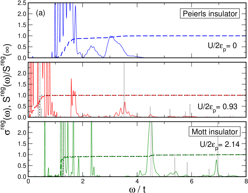
Figure 6: (Color in online edition) (a) The optical conductivity $\sigma^{\text{reg}}(\omega)$ and its integral $S^{\text{reg}}(\omega)$ for the Holstein Hubbard model at half-filling with different ratios of the Coulomb interaction $U$ to the electron-lattice coupling $\varepsilon_{p}=g^{2}\omega_{0}$, $\omega_{0}=0.1t$, and $g^{2}=7$. Black dotted lines denote excitations of the pure Hubbard model. (b) The one-particle spectral function at the transition point, i.e., for the same parameters as in the middle panel of (a). The system size is $L=8$.

The next example of a dynamical correlation function is the optical conductivity. Here the imaginary and real parts of our general correlation functions $\langle A;B\rangle_{\omega}$ change their roles due to an additional frequency integration. The so-called regular contribution to the real part of the optical conductivity is thus given by,

$$\sigma^{\text{reg}}(\omega)=\frac{1}{\omega}\sum_{E_{k}>E_{0}}|\langle k|J|0\rangle|^{2}\ \delta(\omega-(E_{k}-E_{0}))\,,$$ (146)

where the operator

$$J=-\operatorname{i}qt\sum_{i,\sigma}(c_{i,\sigma}^{\dagger}c_{i+1,\sigma}-\text{H.c.})$$ (147)

describes the current. After rescaling the energy and shifting the frequency, $\omega=\tilde{\omega}+\tilde{E}_{0}$, the sum can be expanded as described earlier, now with $J|0\rangle$ as the initial state for the Chebyshev recursion. Back-scaling and dividing by $\omega$ then yields the final result.

In Figure 6 we apply this setup to the Holstein Hubbard model, which is the generalization of the Holstein model to true, spin-carrying electrons that interact via a screened Coulomb interaction, modelled by a Hubbard $U$-term,

$$H=-t\sum_{i,\sigma}(c_{i,\sigma}^{\dagger}c_{i+1,\sigma}+\text{H.c.})+U\sum_{i}n_{i\uparrow}n_{i\downarrow}\\ -g\omega_{0}\sum_{i,\sigma}(b_{i}^{\dagger}+b_{i})n_{i\sigma}+\omega_{0}\sum_{i}b_{i}^{\dagger}b_{i}\,.$$ (148)

For a half-filled band, which now denotes a density of one electron per site, the electronic properties of the model are governed by a competition of two insulating phases: a Peierls (or band) insulator caused by the electron-lattice interaction and a Mott (or correlated) insulator caused by the electron-electron interaction. Within the optical conductivity both phases are signalled by an excitation gap, which closes at the transition between the two phases. We illustrate this behavior in Figure 6 (a), showing $\sigma^{\text{reg}}(\omega)$ at strong electron-phonon coupling and for increasing $U$. The data for the one-particle spectral function in Figure 6 (b) proves that simultaneously to the optical gap also the charge gap vanishes at the quantum phase transition point Fehske et al. (2002, 2004).

III.3.4 Spin structure factor

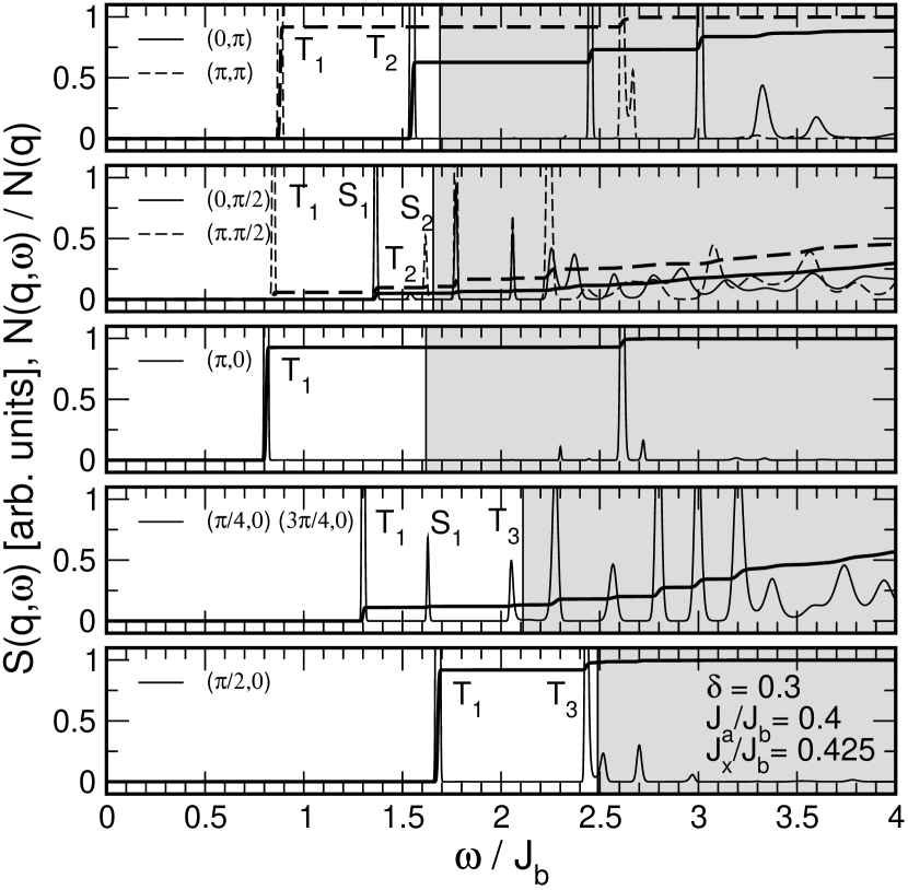
Figure 7: Spin structure factor at $T=0$ calculated for the model (149) which aims at describing the magnetic compound (VO)₂P₂O₇. For more details see Weiße et al. (1999).

Apart from electron systems, of course, the KPM approach works also for other quantum problems such as pure spin systems. To describe the excitation spectrum and the magnetic properties of the compound (VO)₂P₂O₇, some years ago we proposed the 2D spin Hamiltonian Weiße et al. (1999)

$$H=J_{b}\sum_{i,j}(1+\delta(-1)^{i})\vec{S}_{i,j}\cdot\vec{S}_{i+1,j}+J_{a}\sum_{i,j}\vec{S}_{i,j}\cdot\vec{S}_{i,j+1}\\ +J_{\times}\sum_{i,j}(\vec{S}_{2i,j}\cdot\vec{S}_{2i+1,j+1}+\vec{S}_{2i+1,j}\cdot\vec{S}_{2i,j+1})\,,$$ (149)

where $\vec{S}_{i,j}$ denote spin-$1/2$ operators on a square lattice. With this model we aimed at explaining the observation of two branches of low-lying triplet excitations by neutron scattering Garrett et al. (1997), which was inconsistent with the then prevailing picture of (VO)₂P₂O₇ being a spin-ladder or alternating chain compound.

Studying the low-energy physics of the model (149) the KPM approach can be used to calculate the spin structure factor and the integrated spectral weight,

$$S(\vec{q},\omega) =\sum_{k}|\langle k|\vec{S}^{z}(\vec{q})|0\rangle|^{2}\delta(E_{k}-E_{0}-\omega)\,,$$ (150)

$$N(\vec{q},\omega) =\int_{0}^{\omega}d\omega^{\prime}S(\vec{q},\omega^{\prime})\,,$$ (151)

where $\vec{S}^{z}(\vec{q})=\sum_{i,j}\operatorname{e}^{\operatorname{i}\vec{q}\cdot\vec{r}_{i,j}}S^{z}_{i,j}$. Figure 7 shows these quantities for a $4\times 8$ cluster with periodic boundary conditions. The dimension of the sector $S_{z}=0$, which contains the ground state, is rather moderate here being of the order of $D\approx 4\cdot 10^{7}$ only. The expansion clearly resolves the lowest (massive) triplet excitations $T_{1}$, a number of singlets and, in particular, a second triplet branch $T_{2}$. The shaded region marks the two-particle continuum obtained by exciting two of the elementary triplets $T_{1}$, and illustrates that $T_{2}$ is lower in energy. Since the system is finite in size, of course, the continuum appears only as a set of broad discrete peaks, the density of which increases with the system size.

III.4 Dynamical correlations at finite temperature

III.4.1 General considerations

In the preceding section we mentioned briefly that for non-interacting electron systems or for interacting systems at finite temperature the calculation of dynamical correlation functions is more involved, due to the required double summation over all matrix elements of the measured operators. Chebyshev expansion, nevertheless, offers an efficient way for handling these problems. To be specific, let us derive all new ideas on the basis of the optical conductivity $\sigma(\omega)$, which will be our primary application below. Generalizations to other dynamical correlations can be derived without much effort.

For an interacting system the extension of Eq. (146) is given by

$$\sigma^{\text{reg}}(\omega)=\sum_{k,q}\frac{|\langle k|J|q\rangle|^{2}(\operatorname{e}^{-\beta E_{k}}-\operatorname{e}^{-\beta E_{q}})}{ZD\,\omega}\,\delta(\omega-\omega_{qk})\,,$$ (152)

with $\omega_{qk}=E_{q}-E_{k}$. Compared to Eq. (146) a straight-forward expansion of the finite temperature conductivity is spoiled by the presence of the Boltzmann weighting factors. Some authors Iitaka and Ebisuzaki (2003) try to handle this problem by expanding these factors in Chebyshev polynomials and performing a numerical time evolution subsequently, which, however, requires a new simulation for each temperature. A much simpler approach is based on the function

$$j(x,y)=\frac{1}{D}\sum_{k,q}|\langle k|J|q\rangle|^{2}\ \delta(x-E_{k})\ \delta(y-E_{q})$$ (153)

which we may interpret as a matrix element density. Being a function of two variables, $j(x,y)$ can be expanded with two-dimensional KPM,

$$\tilde{j}(x,y)=\sum\limits_{n,m=0}^{N-1}\frac{\mu_{nm}h_{nm}g_{n}g_{m}T_{n}(x)T_{m}(y)}{\pi^{2}\sqrt{(1-x^{2})(1-y^{2})}}$$ (154)

where $\tilde{j}(x,y)$ refers to the rescaled $j(x,y)$, $g_{n}$ are the usual kernel damping factors (see Eq. (71)), and $h_{nm}$ account for the correct normalization (see Eq. (95)). The moments $\mu_{nm}$ are obtained from

$$\mu_{nm} =\int\limits_{-1}^{1}\int\limits_{-1}^{1}\tilde{j}(x,y)T_{n}(x)T_{m}(y)\,dx\,dy$$ (155)

$$=\frac{1}{D}\sum_{k,q}|\langle k|J|q\rangle|^{2}\ T_{n}(\tilde{E}_{k})\ T_{m}(\tilde{E}_{q})$$

$$=\frac{1}{D}\sum_{k,q}\langle k|T_{n}(\tilde{H})J|q\rangle\langle q|T_{m}(\tilde{H})J|k\rangle$$

$$=\frac{1}{D}\operatorname{Tr}\big{(}T_{n}(\tilde{H})JT_{m}(\tilde{H})J\big{)}\,,$$

and again the trace can be replaced by an average over a relatively small number $R$ of random vectors $|r\rangle$. The numerical effort for an expansion of order $n,m<N$ ranges between $2RDN$ and $RDN^{2}$ operations, depending on whether memory is available for up to $N$ vectors of the Hilbert space dimension $D$ or not. Given the operator density $j(x,y)$ we find the optical conductivity by integrating over Boltzmann factors,

$$\sigma^{\text{reg}}(\omega) =\frac{1}{Z\omega}\int\limits_{-\infty}^{\infty}j(y+\omega,y)\big{(}\operatorname{e}^{-\beta y}-\operatorname{e}^{-\beta(y+\omega)}\big{)}\,dy$$ (156)

$$=\sum_{k,q}\frac{|\langle k|J|q\rangle|^{2}(\operatorname{e}^{-\beta E_{k}}-\operatorname{e}^{-\beta E_{q}})}{ZD\omega}\,\delta(\omega-\omega_{qk})\,,$$

and, as above, we get the partition function $Z$ from an integral over the density of states $\rho(E)$. The latter can be expanded in parallel to $j(x,y)$. Note that the calculation of the conductivity at different temperatures is based on the same operator density $j(x,y)$, i.e., it needs to be expanded only once for all temperatures.

Surprisingly, the basic steps of this approach were suggested already ten years ago Wang and Zunger (1994); Wang (1994), but — probably overlooking its potential — applied only to the zero-temperature response of non-interacting electrons. A reason for the poor appreciation of these old ideas may also lie in the use of non-optimal kernels, which did not ensure the positivity of $j(x,y)$ and reduced the numerical precision. Only recently, one of the authors generalized the Jackson kernel and obtained high resolution optical data for the Anderson model Weiße (2004). More results, in particular for interacting quantum systems at finite temperature, we present hereafter.

III.4.2 Optical conductivity of the Anderson model

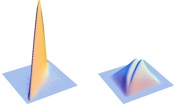
Figure 8: (Color in online edition) The matrix element density $j(x,y)$ for the 3D Anderson model with disorder $W/t=2$ and $12$.

Since the Anderson model describes non-interacting fermions, the eigenstates $|k\rangle$ occurring in $\sigma(\omega)$ now denote single-particle wave functions and the Boltzmann weight has to be replaced by the Fermi function,

$$\sigma^{\text{reg}}(\omega) =\frac{1}{\omega}\int\limits_{-\infty}^{\infty}j(y+\omega,y)\big{(}f(y)-f(y+\omega)\big{)}\,dy$$ (157)

$$={\sum_{k,q}}\frac{|\langle k|J|q\rangle|^{2}(f(E_{k})-f(E_{q}))}{\omega}\,\delta(\omega-\omega_{qk})\,.$$

Clearly, from a computational point of view this expression is of the same complexity for both, zero and finite temperature, and indeed, compared to Sec. III.3, we need the more advanced 2D KPM approach.

Figure 8 shows the matrix element density $j(x,y)$ calculated for the 3D Anderson model on a $D=50^{3}$ site cluster. The expansion order is $N=64$, and the moment data was averaged over $S=10$ disorder samples and $R=10$ random start vectors each. Starting from a “shark fin” at weak disorder, with increasing $W$ the density $j(x,y)$ spreads in the entire energy plane, simultaneously developing a sharp dip along $x=y$. A comparison with Eq. (157) reveals that this dip is responsible for the decreasing and finally vanishing DC conductivity of the model Weiße (2004). In Figure 9 we show the resulting optical conductivity at $W/t=12$ for different chemical potentials $\mu$ and temperatures $\beta=1/T$. Note that all curves are derived from the same matrix element density $j(x,y)$, which is now based on a $D=100^{3}$ site cluster, expansion order $N=2048$, an average over $S=440$ samples and only $R=1$ random start vectors each.

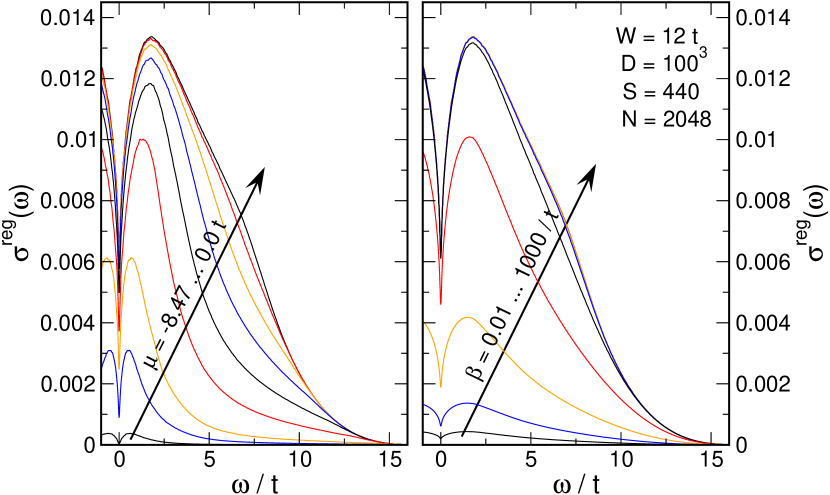
Figure 9: (Color in online edition) Optical conductivity of the 3D Anderson model at disorder $W=12$ and for different chemical potentials $\mu$ and temperatures $\beta=1/T$.

III.4.3 Optical conductivity of the Holstein model

Having discussed dynamical correlations for non-interacting electrons, let us now come back to the case of interacting systems. The setup described so far works well for high temperatures, but as soon as $T$ gets small we experience the same problems as with thermal expectation values and static correlations. Again, the Boltzmann factors put most of the weight to the margins of the domain of $j(x,y)$, thus amplifying small numerical errors. To properly approach the limit $T\to 0$ we therefore have to separate the ground state and a few lowest excitations from the rest of the spectrum in a fashion similar to the static correlations in Sec. III.2. Since we start from a 2D expansion, the correlation function (optical conductivity) now splits into three parts: a contribution from the transitions (or matrix elements) between the separated eigenstates, a sum of 1D expansions for the transitions between the separated states and the rest of the spectrum (see Sec. III.3), and a 2D expansion for all transitions within the rest of the spectrum,

$$\sigma^{\text{reg}}(\omega)=\underbrace{\sum_{k,q=0}^{C-1}\sigma_{k,q}}_{\sigma^{\text{reg}}_{\text{ED}}(\omega)}+\underbrace{\sum_{k=0}^{C-1}\sum_{q=C}^{D-1}(\sigma_{k,q}+\sigma_{q,k})}_{\sigma^{\text{reg}}_{\text{1D}}(\omega)}+\underbrace{\sum_{k,q=C}^{D-1}\sigma_{k,q}}_{\sigma^{\text{reg}}_{\text{2D}}(\omega)}\,,$$ (158)

with

$$\sigma_{k,q}=\frac{|\langle k|J|q\rangle|^{2}(\operatorname{e}^{-\beta E_{k}}-\operatorname{e}^{-\beta E_{q}})\,\delta(\omega-\omega_{qk})}{ZD\omega}\,.$$ (159)

The expansions required for $\sigma^{\text{reg}}_{\text{1D}}(\omega)$ are carried out in analogy to Sec. III.3.3, but the resulting conductivities are weighted appropriately when all contributions are combined to $\sigma^{\text{reg}}(\omega)$. Using the projection operator defined in Eq. (131), the corresponding moments read

$$\mu_{n}^{k}=\langle k|JPT_{n}(\tilde{H})PJ|k\rangle\,.$$ (160)

For $\sigma^{\text{reg}}_{\text{2D}}(\omega)$ we follow the scheme outlined in III.4.1, but use projected moments

$$\mu_{nm}=\operatorname{Tr}(T_{n}(\tilde{H})PJT_{m}(\tilde{H})PJ)/D\,.$$ (161)

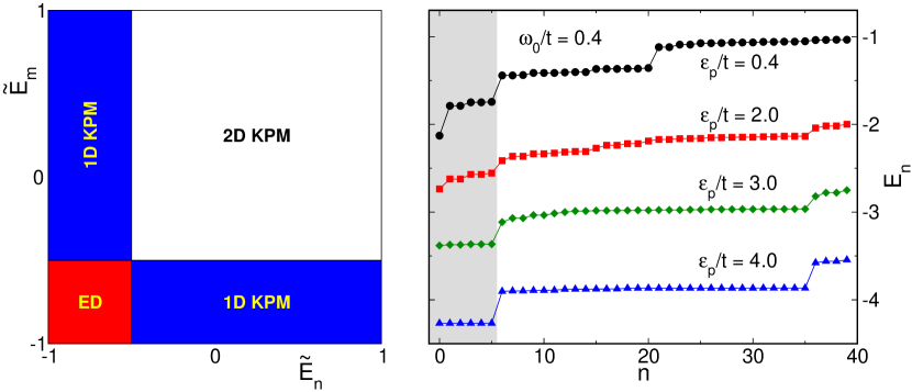
Figure 10: (Color in online edition) Left: Schematic setup for the calculation of finite-temperature dynamical correlations for interacting quantum systems, which requires a separation into parts handled by exact diagonalization (ED), 1D Chebyshev expansion and 2D Chebyshev expansion. Right: The lowest eigenvalues of the Holstein model on a six site chain for different electron-phonon coupling $\varepsilon_{p}$. The shaded region marks the lowest polaron band, which was handled separately when calculating the spectra in Figure 11.

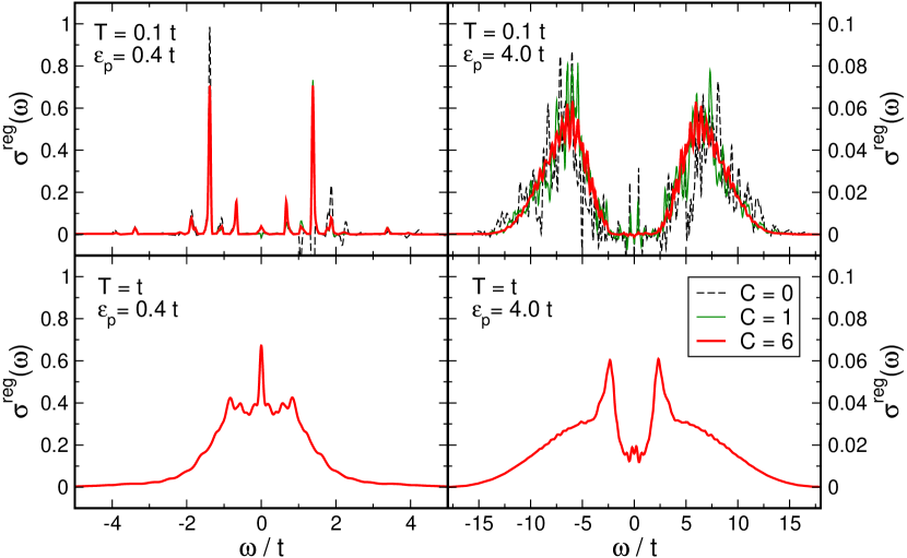
Figure 11: (Color in online edition) Finite temperature optical conductivity of a single electron coupled to the lattice via a Holstein type interaction. Different colors illustrate how, in particular, the low-temperature spectra benefit from a separation of $C=0,1$ or $6$ low-energy states Schubert et al. (2005c). The phonon frequency is $\omega_{0}/t=0.4$.

In Figure 10 we illustrate our setup schematically and show the lowest forty eigenvalues of the Holstein model, Eq. (143), with a band filling of one electron. Separating up to six states from the rest of the spectrum we obtain the finite-temperature optical conductivity of the system, Figure 11. For high temperatures ($T=t$, see lower panels) the separation of low-energy states is not necessary, the conductivity curves for $C=0,1$ and $6$ agree very well. For low temperatures ($T=0.1t$, see upper panels), the separation is crucial. Without any separated states ($C=0$) the conductivity has substantial numerical errors and can even become negative, if large Boltzmann factors amplify infinitesimal numerical round-off errors of negative sign. Splitting off the ground state ($C=1$) or the entire (narrow) polaron band ($C=6$ for the present six-site cluster), we obtain reliable, high-resolution spectra down to the lowest temperatures. From a physics point of view, at strong electron phonon coupling (right panels) the conductivity shows an interesting transfer of spectral weight from high to low frequencies, if the temperature is increased (see Schubert et al. (2005c) for more details).

With this discussion of optical conductivity as a finite temperature dynamical correlation function we conclude the section on direct applications of KPM. Of course, the described techniques can be used for the solution of many other interesting and numerically demanding problems, but an equally important field of applications emerges, when KPM is embedded into other numerical or analytical techniques, which is the subject of the next section.

IV KPM as a component of other methods

IV.1 Monte Carlo simulations

In condensed matter physics some of the most intensely studied materials are affected by a complex interplay of many degrees of freedom, and when deriving suitable approximate descriptions we frequently arrive at models, where non-interacting fermions are coupled to classical degrees of freedom. Examples are colossal magneto-resistant manganites Dagotto (2003) or magnetic semiconductors Schliemann et al. (2001), where the classical variables correspond to localized spin degrees of freedom. We already introduced such a model when we discussed the limit $S\to\infty$ of the double-exchange model, Eq. (117). The properties of these systems, e.g. a ferromagnetic ordering as a function of temperature, can be studied by standard MC procedures. However, in contrast to purely classical systems the energy of a given spin configuration, which enters the transition probabilities, cannot be calculated directly, but requires the solution of the corresponding non-interacting fermion problem. This is usually the most time consuming part, and an efficient MC algorithm should therefore evaluate the fermionic trace as fast and as seldom as possible.

The first requirement can be matched by using KPM for calculating the density of states of the fermion system, which by integration over the Fermi function yields the energy of the underlying spin configuration. Combined with standard Metropolis single-spin updates this led to the first MC simulations of double-exchange systems Motome and Furukawa (1999, 2000, 2001) on reasonably large clusters ($8^{3}$ sites), which were later improved by replacing full traces by trace estimates and by increasing the efficiency of the matrix vector multiplications Furukawa and Motome (2004); Alvarez et al. (2005).

To fulfil the second requirement it would be advantageous to replace the above single-spin updates by updates of the whole spin background. The first implementation of such ideas was given in terms of an hybrid Monte Carlo algorithm Alonso et al. (2001), which combines an approximate time evolution of the spin system with a diagonalization of the fermionic problem by Legendre expansion, and requires a much smaller number of MC accept-reject steps. However, this approach has the drawback of involving a molecular dynamics type simulation of the classical degrees of freedom, which is a bit complicated and which may bias the system in the direction of the assumed approximate dynamics.

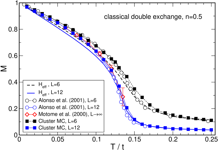
Figure 12: (Color in online edition) Magnetization as a function of temperature for the classical double-exchange model at doping $n=0.5$. We compare data obtained from the effective model $H_{\text{eff}}$ (see text), from a hybrid Monte Carlo approach Alonso et al. (2001), the Truncated Polynomial Expansion Method Motome and Furukawa (2000, 2001), and from a KPM based Cluster Monte Carlo technique Weiße et al. (2005). $L$ denotes the size of the underlying three-dimensional cluster, i.e., $D=L^{3}$ is the dimension of the fermionic problem.

Focussing on the problem of classical double exchange, Eq. (117), we therefore proposed a third approach Weiße et al. (2005), which combines the advantages of KPM with the highly efficient Cluster MC algorithms Wolff (1989); Janke (1998); Krauth (2004). In general, for a classical MC algorithm the transition probability from state $a$ to state $b$ can be written as

$$P(a\to b)=A(a\to b)\tilde{P}(a\to b)\,,$$ (162)

where $A(a\to b)$ is the probability of considering the move $a\to b$, and $\tilde{P}(a\to b)$ is the probability of accepting the move $a\to b$. Given the Boltzmann weights of the states $a$ and $b$, $W(a)$ and $W(b)$, detailed balance requires that

$$W(a)P(a\to b)=W(b)P(b\to a)\,,$$ (163)

which can be fulfilled with a generalized Metropolis algorithm

$$\tilde{P}(a\to b)=\min\left(1,\frac{W(b)A(b\to a)}{W(a)A(a\to b)}\right)\,.$$ (164)

In the standard MC approach for spin systems only a single randomly chosen spin is flipped. Hence, $A(a\to b)=A(b\to a)$ and the probability $\tilde{P}(a\to b)$ is usually much smaller than $1$, since it depends on temperature via the weights $W(a)$ and $W(b)$. This disadvantage can be avoided by a clever construction of clusters of spins, which are flipped simultaneously, such that the a priori probabilities $A(a\to b)$ and $A(b\to a)$ soak up any difference in the weights $W(a)$ and $W(b)$. We then arrive at the famous rejection-free cluster MC algorithms Wolff (1989), which are characterized by $\tilde{P}(a\to b)=1$.

For the double-exchange model (117) we cannot expect to find an algorithm with $\tilde{P}(a\to b)=1$, but even a method with $\tilde{P}(a\to b)=0.5$ would be highly efficient. The amplitude of the hopping matrix element (118) is given by the cosine of half the relative angle between neighboring spins, or $|t_{ij}|^{2}=(1+\vec{S}_{i}\cdot\vec{S}_{j})/2$. Averaging over the fermionic degrees of freedom, we thus arrive at an effective classical spin model

$$H_{\text{eff}}=-J_{\text{eff}}\sum_{\langle ij\rangle}\sqrt{1+\vec{S}_{i}\cdot\vec{S}_{j}}\,,$$ (165)

where the particle density $n$ approximately defines the coupling, $J_{\text{eff}}\approx n(1-n)/\sqrt{2}$. Similar to a classical Heisenberg model, the Hamiltonian $H_{\text{eff}}$ is a sum over contributions of single bonds, and we can therefore construct a cluster algorithm with $\tilde{P}(a\to b)=1$. Surprisingly, the simulation of this pure spin model yields magnetization data, which almost perfectly matches the results for the full classical double-exchange model at doping $n=0.5$, see Figure 12.

For simulating the coupled spin fermion model (117) we suggested to apply the single cluster algorithm for $H_{\text{eff}}$ until approximately every spin in the system has been flipped once, thereby keeping track of all a priori probabilities $A(a\to b)$ of subsequent cluster flips. Then for the new spin configuration the energy of the electron system is evaluated with the help of KPM. Note however, that for a reliable discrimination of $H_{\text{eff}}$ and the full fermionic model (117) the energy calculation needs to be very precise. For the moment calculation we therefore relied on complete trace summations instead of stochastic estimates. The KPM step is thus no longer linear in $D$, but still much faster than a full diagonalization of the bilinear fermionic model. Based on the resulting energy, the new spin configuration is accepted with the probability (164). Figure 12 shows the magnetization of the double-exchange model as a function of temperature for $n=0.5$. Except for small deviations near the critical temperature the data obtained with the new approach compares well with the results of the hybrid MC approach Alonso et al. (2001), and due to the low numerical effort rather large systems can be studied.

Of course, the combination of KPM and classical Monte Carlo not only works for spin systems. We may also think of models involving the coupling of electronic degrees of freedom to adiabatic lattice distortions or other classical variables Alvarez et al. (2005), and as yet the potential of such combined approaches is certainly not fully exhausted.

The next application, which makes use of KPM as a component of a more general numerical approach, brings us back to interacting quantum systems, in particular, correlated electron systems with strong local interactions.

IV.2 Cluster Perturbation Theory (CPT)

IV.2.1 General features of CPT

Earlier in this review we have demonstrated the advantages of the Chebyshev approach for the calculation of spectral functions, optical conductivities and structure factors of complicated interacting quantum systems. However, owing to the finite size of the considered systems, quantities like the spectral function $A(\vec{k},\omega)$ could only be calculated for a finite set of independent momenta $\vec{k}$. The interpretation of this “discrete” data may sometimes be less convenient, e.g. the $\vec{k}$-integrated one-electron density $\rho(\omega)=\int dk^{d}\,A(\vec{k},\omega)$ does not show bands but only discrete poles which are grouped to band-like structures. Although this does not substantially bias the interpretation it is desirable to restore the translational symmetry of the lattice and reintroduce an infinite momentum space.

With the Cluster Perturbation Theory (CPT) Gros and Valentí (1994); Sénéchal et al. (2000, 2002) a straightforward way to perform this task approximatively has recently been devised. To describe it in a nutshell, let us consider a model of interacting fermions on a one-dimensional chain

$$H=-t\sum_{i\sigma}(c^{\dagger}_{i+1,\sigma}c_{i,\sigma}+\text{H.c.})+\sum_{i}U_{i}\,.$$ (166)

Here $U_{i}$ denotes a local interaction, e.g. $U_{i}=Un_{i\uparrow}n_{i\downarrow}$ for the Hubbard model. CPT starts by breaking up the infinite system into short finite chains of $L$ sites each (clusters), which all are equivalent due to translational symmetry. From the Green function of a finite chain, $G^{c}_{ij}(\omega)$ with $i,j=0,\dots,L-1$, which is calculated exactly by a suitable numerical method, the Green function $G(k,\omega)$ of the infinite chain is obtained by reintroducing the hopping between the segments. This inter-chain hopping is treated on the level of a random phase approximation, which neglects correlations between different chains. The Green function $G_{ij}^{nm}(\omega)$ is then given through a Dyson equation

$$G_{ij}^{nm}(\omega)=\delta_{nm}G^{c}_{ij}(\omega)+\sum\limits_{i^{\prime},j^{\prime},m^{\prime}}G^{c}_{ii^{\prime}}(\omega)V_{i^{\prime}j^{\prime}}^{nm^{\prime}}G_{j^{\prime}j}^{m^{\prime}m}(\omega)\,,$$ (167)

where $V_{ij}^{nm}=-t(\delta_{n,m+1}\delta_{i0}\delta_{j,L-1}+\delta_{n,m-1}\delta_{i,L-1}\delta_{j0})$ describes the inter-chain hopping and upper indices number the different clusters. A partial Fourier transform of the inter-chain hopping, $V_{ij}(Q)=-t(\operatorname{e}^{\operatorname{i}Q}\delta_{i0}\delta_{j,L-1}+\operatorname{e}^{-\operatorname{i}Q}\delta_{i,L-1}\delta_{j0})$, gives the infinite-lattice Green function in a mixed representation

$$\hat{G}_{ij}(Q,\omega)=\left(\frac{G^{c}(\omega)}{1-V(Q)G^{c}(\omega)}\right)_{ij}$$ (168)

for a momentum vector $Q$ of the super-lattice of finite chains and cluster indices $i,j$. Finally, from this mixed representation the infinite lattice Green function in momentum space is recovered in the CPT approximation as a simple Fourier transform

$$G(k,\omega)=\frac{1}{L}\sum\limits_{i,j}\exp(\operatorname{i}(i-j)k)\,\hat{G}_{ij}(Lk,\omega)\,.$$ (169)

The reader should be aware that restoring translational symmetry in the CPT sense is different from performing the thermodynamic limit of the interacting system. The CPT may be understood as a kind of interpolation scheme from the discrete momentum space of a finite cluster to the continuous $\vec{k}$-values of the infinite lattice. The amount of information attainable from the solution of a finite cluster problem does however not increase. Especially finite-size effects affecting the interaction properties are by no means reduced, but still determined through the size of the underlying cluster. Nevertheless, CPT yields appealing presentations of the finite-cluster data, which can ease its interpretation.

At present, all numerical studies within the CPT context use Lanczos recursion for the cluster diagonalization, thus suffering from the shortcomings we discussed earlier. As an alternative, we prefer to use the formalism introduced in Sec. III.3, which is much better suited for the calculation of spectral properties in a finite energy interval.

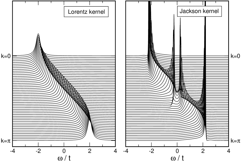
Figure 13: Spectral function for non-interacting tight-binding electrons. Based on the Lorentz kernel CPT exactly reproduces the infinite system result (left), the Jackson kernel does not have the correct analytical properties, therefore CPT cannot close the finite size gap at $k=\pi/2$ (right).

On applying the CPT crucial attention has to be paid to the kernel used in the reconstruction of $G^{c}_{ij}(\omega)$. As it turns out, the Jackson kernel is an inadequate choice here, since already for the non-interacting tight-binding model it introduces spurious structures into the spectra. The failure can be attributed to the shape of the Jackson kernel: Being optimized for high resolution, a pole in the Green function will give a sharp peak with most of its weight concentrated at the center, and rapidly decaying tails. The reconstructed (cluster) Green function therefore does not satisfy the correct analytical properties required in the CPT step. To guarantee these properties, instead, we use the Lorentz kernel, which we constructed in Sec. II.3.4 to mimic the effect of a finite imaginary part in the energy argument of a Green function. Using this kernel for the reconstruction of $G^{c}_{ij}(\omega)$ the CPT works perfectly (cf. Figure 13).

To provide further examples we present results for two different interacting models where the cluster Green function $G^{c}_{ij}(\omega)$ has been calculated through a Chebyshev expansion as in Eq. (140). Using $G^{c}_{ij}(\omega)=G^{c}_{ji}(\omega)$ (no magnetic field), for a $L$-site chain $L$ diagonal and $L(L-1)/2$ off-diagonal elements of $G^{c}_{ij}(\omega)$ have to be calculated. The latter can be reduced to Chebyshev iterations for the operators $c_{i}^{(\dagger)}+c_{j}^{(\dagger)}$, which allows application of the “doubling trick” (see the remark after Eq. (138)). However, the numerical effort can be further reduced by a factor $1/L$: If we keep the ground state $|0\rangle$ of the system we can calculate the moments $\mu^{ij}_{n}=\langle 0|c_{i}T_{n}(\tilde{H})c^{\dagger}_{j}|0\rangle$ for $L$ elements $i=1,\dots,L$ of $G^{c}_{ij}(\omega)$ in a single Chebyshev iteration. To achieve a similar reduction within the Lanczos recursion we had to explicitly construct the eigenstates to the Lanczos eigenvalues. Then the factor $1/L$ is exceeded by at least $ND$ additional operations for the construction of $N$ eigenstates of a $D$-dimensional sparse matrix. Hence using KPM for the CPT cluster diagonalization the numerical effort can be reduced by a factor of $1/L$ in comparison to the Lanczos recursion.

IV.2.2 CPT for the Hubbard model

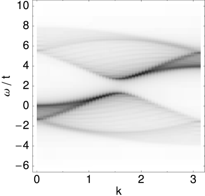
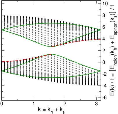
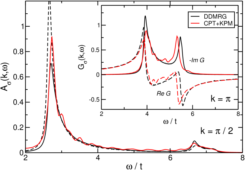
Figure 14: (Color in online edition) Spectral function of the 1D Hubbard model for half-filling and $U=4t$. Top left: CPT result with cluster size $L=16$ and expansion order $N=2048$. For similar data based on Lanczos recursion see Sénéchal et al. (2000). Top right: Within the exact Bethe ansatz solution each electron separates into the sum of independent spinon (red dashed) and holon (green) excitations. The dots mark the energies of a 64-site chain. Bottom: CPT data compared to selected DDMRG results for a system with $L=128$ sites, open boundary conditions and a broadening of $\epsilon=0.0625t$. Note that in DDMRG the momenta are approximate.

As a first example we consider the 1D Hubbard model (Eq. (148) with $g=\omega_{0}=0$), which is exactly solvable by Bethe ansatz Essler et al. (2005) and was also extensively studied with DDMRG Jeckelmann et al. (2000). It thus provides the opportunity to assess the precision of the KPM-based CPT. The top left panel of Figure 14 shows the one-particle spectral function at half-filling, calculated on the basis of $L=16$ site clusters and an expansion order of $N=2048$. The matrix dimension is $D\approx 1.7\cdot 10^{8}$. Remember that the cluster Green function is calculated for a chain with open boundary conditions. The reduced symmetry compared to periodic boundary conditions results in a larger dimension of the Hilbert space that has to be dealt with numerically. In the top right panel the dots show the Bethe ansatz results for a $L=64$ site chain, and the lines denote the $L\to\infty$ spinon and holon excitations each electron separates into (spin-charge separation). So far the Bethe ansatz does not allow for a direct calculation of the structure factor, the data thus represents only the position and density of the eigenstates, but is not weighted with the matrix elements of the operators $c_{k\sigma}^{(\dagger)}$. Although for an infinite system we would expect a continuous response, the CPT data shows some faint fine-structure. A comparison with the finite-size Bethe ansatz data suggests that these features are an artifact of the finite-cluster Greens function which the CPT spectral function is based on. The fine-structure is also evident in the lower panel of Figure 14, where we compare with DDMRG data for a $L=128$ site system. Otherwise the CPT nicely reproduces all expected features, like the excitation gap, the two pronounced spinon and holon branches, and the broad continuum. Note also, that CPT is applicable to all spatial dimensions, whereas DDMRG works well only for 1D models.

IV.2.3 CPT for the Holstein model

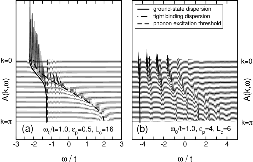
Figure 15: Spectral function $A^{+}(k,\omega)$ of a single electron in the Holstein model (corresponding to $N_{\text{e}}=0$ in Eq. (145)). For weak electron-phonon coupling the original band is still very pronounced (left), for intermediate-to-strong coupling many narrow polaron bands develop (right). The cluster size is $L=16$ (left) or $L=6$ (right) and the expansion order $N=2048$. See Hohenadler et al. (2003) for similar data based on Lanczos recursion.

Our second example is the spectral function of a single electron in the Holstein model, i.e., Eq. (148) with $U=0$. Here, as a function of the electron-phonon interaction, polaron formation sets in and the band width of the resulting quasi particles becomes extremely narrow at large coupling strength. Figure 15 illustrates this behavior for two values of the electron-phonon coupling $\varepsilon_{p}=g^{2}\omega_{0}$. For weak coupling the original one-electron band is still clearly visible (dot-dashed line), but the dispersion-less phonon (dashed line) cuts in approximately at an energy $\omega_{0}$ above the band minimum, causing the formation of a polaron band (solid line; calculated with the approach of Bonča et al. (1999)), an avoided-crossing like gap and a number of finite-size features. For strong coupling the spectral weight of the electron is distributed over many narrow polaron bands separated approximately by the bare phonon frequency $\omega_{0}$.

In all these cases, KPM works as a reliable high-resolution cluster solver, and using the concepts from Sec. III.4 we could also extend these calculations to finite temperature. Probably, CPT is not the only approximate technique that profits from the simplicity and stability of KPM, and the range of its applications can certainly be extended.

V KPM versus other numerical approaches

After we have given a very detailed description of the Kernel Polynomial Method and presented a wide range of applications, let us now classify the method in the context of numerical many-particle techniques and comment on a number of other numerical approaches that are closely related to KPM.

V.1 KPM and dedicated many-particle techniques

In the previous sections we already compared KPM data and results of other numerical many-particle techniques. Nevertheless, it seems appropriate to add a few comments about the general concept of such calculations and the role KPM-like methods play in the field of many-particle physics and complex quantum systems. The numerical study of interacting quantum many-particle systems is complicated by the huge Hilbert space dimensions involved, which usually grow exponentially with the number of particles or the system size. There are different strategies to cope with this: In Monte Carlo approaches only part of the Hilbert space is sampled stochastically, thereby trying to capture the essential physics with an appropriate weighting mechanism. On the other hand, variational methods, like DMRG Peschel et al. (1999); Schollwöck (2005) or the specialized approach of Bonča et al. (1999), aim at reducing the Hilbert space dimension in an intelligent way by discarding unimportant states, which, for instance, contribute only at high temperature. Compared to such methods KPM is much more basic: It is designed only for the fast and stable calculation of the spectral properties of a given matrix and of related correlations. Choosing a suitable Hilbert space or optimizing the basis is the matter of the user or of external programs. It is thus a more general approach, which can be used directly or embedded into other methods, as we illustrated in the preceding section. Of course, this simplicity and general applicability come at a certain price: For interacting many-particle models the system sizes that can be studied by using KPM directly are usually much smaller, compared to DMRG and Monte Carlo. Note however, that both of the latter methods have limitations too: For many interesting models Monte Carlo methods are plagued by the infamous sign problem, which is not present in KPM. When it comes to the calculation of dynamical correlation functions Monte Carlo approaches rely on power moments. The reconstruction of correlation functions from power moments is known to be an ill-conditioned problem, in particular, if the moments are subject to statistical noise. The resolution of Monte Carlo results is therefore much smaller compared to the data obtained with KPM. The DMRG method develops its full potential only in one spatial dimension and for short ranged interactions. In addition, the calculation of dynamical correlations is limited to zero temperature, with only a few exceptions Sirker and Klümper (2005). None of these restrictions apply to KPM.

V.2 Close relatives of KPM

Having compared KPM to specialized many-particle methods, let us now discuss more direct competitors of KPM, i.e., methods that share the broad application range and some of its general concepts.

V.2.1 Chebyshev expansion and Maximum Entropy Methods

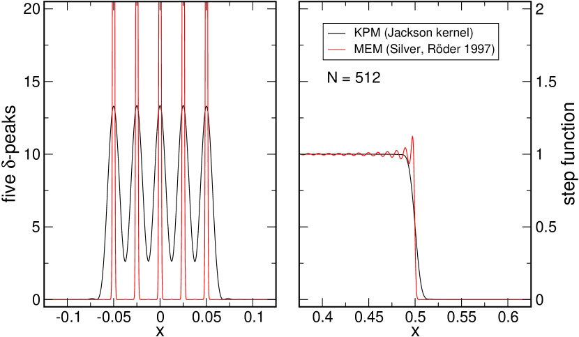
Figure 16: (Color in online edition) Comparison of a KPM and a MEM approximation to a spectrum consisting of five isolated $\delta$-peaks, and to a step function. The expansion order is $N=512$. Clearly, for the $\delta$-peaks MEM yields a higher resolution, but for the step function the Gibbs oscillations return.

The first of these approaches, the combination of Chebyshev expansion and Maximum Entropy (MEM), is basically an alternative procedure to transform moment data $\mu_{n}$ into convergent approximations of the considered function $f(x)$. To achieve this, instead of (or in addition to) applying kernel polynomials, an entropy

$$S(f,f_{0})=\int_{-1}^{1}(f(x)-f_{0}(x)-\log(f(x)/f_{0}(x)))\,dx$$ (170)

is maximized under the constraint that the moments of the estimated $f(x)$ agree with the given data. The function $f_{0}(x)$ describes our initial knowledge about $f(x)$, and may in the worst case just be a constant. Being related to Maximum Entropy approaches to the classical moment problem Mead and Papanicolaou (1984); Turek (1988), for the case of Chebyshev moments different implementations of the method have been suggested Skilling (1988); Silver and Röder (1997); Bandyopadhyay et al. (2005). Since for a given set of $N$ moments $\mu_{n}$ the approximation to the function $f(x)$ is usually not restricted to a polynomial of degree $N-1$, compared to the KPM with Jackson kernel the Maximum Entropy approach usually yields estimates of higher resolution. However, this higher resolution results from adding a priori assumptions and not from a true information gain (see also Figure 16). The resource consumption of Maximum Entropy is generally much higher than the $N\log N$ behavior we found for KPM. In addition, the approach is non-linear in the moments and can occasionally become unstable for large $N$. Note also that as yet Maximum Entropy methods have been derived only for positive quantities, $f(x)>0$, such as densities of states or strictly positive correlation functions.

Maximum Entropy, nevertheless, is a good alternative to KPM, if the calculation of the $\mu_{n}$ is particularly time consuming. Based on only a moderate number of moments it yields very detailed approximations of $f(x)$, and we obtained very good results for some computationally demanding problems Bäuml et al. (1998).

V.2.2 Lanczos recursion

Chebyshev / KPM	complexity	Lanczos recursion	complexity
Initialization: $$\displaystyle\tilde{H}=(H-b)/a$$ $$\displaystyle|\phi_{0}\rangle=A|0\rangle,\quad|\phi_{1}\rangle=\tilde{H}|\phi_{0}\rangle$$ $$\displaystyle\mu_{0}=\langle\phi_{0}|\phi_{0}\rangle,\quad\mu_{1}=\langle\phi_{1}|\phi_{0}\rangle$$		Initialization: $$\displaystyle\beta_{0}=\sqrt{\langle 0|A^{\dagger}A|0\rangle}$$ $$\displaystyle|\phi_{0}\rangle=A|0\rangle/\beta_{0},\quad|\phi_{-1}\rangle=0$$
Recursion for $2N$ moments $\mu_{n}$: $$\displaystyle|\phi_{n+1}\rangle=2\tilde{H}|\phi_{n}\rangle-|\phi_{n-1}\rangle$$ $$\displaystyle\mu_{2n+2}=2\langle\phi_{n+1}|\phi_{n+1}\rangle-\mu_{0}$$ $$\displaystyle\mu_{2n+1}=2\langle\phi_{n+1}|\phi_{n}\rangle-\mu_{1}$$	$O(ND)$	Recursion for $N$ coefficients $\alpha_{n}$, $\beta_{n}$: $$\displaystyle|\phi^{\prime}\rangle=H|\phi_{n}\rangle-\beta_{n}|\phi_{n-1}\rangle,\quad\alpha_{n}=\langle\phi_{n}|\phi^{\prime}\rangle$$ $$\displaystyle|\phi^{\prime\prime}\rangle=|\phi^{\prime}\rangle-\alpha_{n}|\phi_{n}\rangle,\quad\beta_{n+1}=\sqrt{\langle\phi^{\prime\prime}|\phi^{\prime\prime}\rangle}$$ $$\displaystyle|\phi_{n+1}\rangle=|\phi^{\prime\prime}\rangle/\beta_{n+1}$$	$O(ND)$
$\to$ very stable		$\to$ tends to lose orthogonality
Reconstruction in three simple steps: Apply kernel: $\tilde{\mu}_{n}=g_{n}\mu_{n}$ Fourier transform: $\tilde{\mu}_{n}\to\tilde{f}(\tilde{\omega}_{i})$ Rescale: $f(\omega_{i})=\dfrac{\tilde{f}[(\omega_{i}-b)/a]}{\pi\sqrt{a^{2}-(\omega_{i}-b)^{2}}}$	$O(M\log M)$	Reconstruction via continued fraction $$\displaystyle f(z)=-\frac{1}{\pi}\operatorname{Im}\cfrac{\beta_{0}^{2}}{z-\alpha_{0}-\cfrac{\beta_{1}^{2}}{z-\alpha_{1}-\cfrac{\beta_{2}^{2}}{z-\alpha_{2}-\ldots}}}$$ $$\displaystyle\text{where }z=\omega_{i}+\operatorname{i}\epsilon$$	$O(NM)$
$\to$ procedure is linear in $\mu_{n}$		$\to$ procedure is non-linear in $\alpha_{n}$, $\beta_{n}$
$\to$ well defined resolution $\propto 1/N$		$\to$ $\epsilon$ is somewhat arbitrary

Table 2: Comparison of Chebyshev expansion and Lanczos recursion for the calculation of a zero-temperature dynamical correlation function $f(\omega)=\sum_{n}|\langle n|A|0\rangle|^{2}\delta(\omega-\omega_{n})$. We assume $N$ matrix vector multiplications with a $D$-dimensional sparse matrix $H$, and a reconstruction of $f(\omega)$ at $M$ points $\omega_{i}$.

The Lanczos Recursion Method is certainly the most capable competitor of the Kernel Polynomial Method Dagotto (1994). It is based on the Lanczos algorithm Lanczos (1950), a method which was initially developed for the tridiagonalization of Hermitian matrices and later evolved to one of the most powerful methods for the calculation of extremal eigenstates of sparse matrices Cullum and Willoughby (1985). Although ideas like the mapping of the classical moment problem to tridiagonal matrices and continued fractions have been suggested earlier Gordon (1968), the use of the Lanczos algorithm for the characterization of spectral densities Haydock et al. (1972, 1975) was first proposed at about the same time as the Chebyshev expansion approaches, and in principle Lanczos recursion is also a kind of modified moment expansion Lambin and Gaspard (1982); Benoit et al. (1992). Its generalization from spectral densities to zero temperature dynamical correlation functions was first given in terms of continued fractions Gagliano and Balseiro (1987), and later also an approach based on the eigenstates of the tridiagonal matrix was introduced and termed Spectral Decoding Method Zhong et al. (1994). This technique was then generalized to finite temperature Jaklič and Prelovšek (1994, 2000), and, in addition, some variants of the approach for low temperature Aichhorn et al. (2003) and based on the micro-canonical ensemble Long et al. (2003) have been proposed recently.

To give an impression, in Table 2 we compare the setup for the calculation of a zero temperature dynamical correlation function within the Chebyshev and the Lanczos approach. The most time consuming step for both methods is the recursive construction of a set of vectors $|\phi_{n}\rangle$, which in terms of scalar products yield the moments $\mu_{n}$ of the Chebyshev series or the elements $\alpha_{n}$, $\beta_{n}$ of the Lanczos tridiagonal matrix. In terms of the number of operations the Chebyshev recursion has a small advantage, but, of course, the application of the Hamiltonian as the dominant factor is the same for both methods. As a drawback, at high expansion order the Lanczos iteration tends to lose the orthogonality between the vectors $|\phi_{n}\rangle$, which it intends to establish by construction. When the Lanczos algorithm is applied to eigenvalue problems this loss of orthogonality usually signals the convergence of extremal eigenstates, and the algorithm then starts to generate artificial copies of the converged states. For the calculation of spectral densities or correlation functions this means that the information content of the $\alpha_{n}$ and $\beta_{n}$ does no longer increase proportionally to the number of iterations. Unfortunately, this deficiency can only be cured with more complex variants of the algorithm, which also increase the resource consumption. Chebyshev expansion is free from such defects, as there is a priori no orthogonality between the $|\phi_{n}\rangle$.

The reconstruction of the considered function from its moments $\mu_{n}$ or coefficients $\alpha_{n}$, $\beta_{n}$, respectively, is also faster and simpler within the KPM, as it makes use of Fast Fourier Transformation. In addition, the KPM is a linear transformation of the moments $\mu_{n}$, a property we used extensively above when averaging moment data instead of the corresponding functions. Continued fractions, in contrast, are non-linear in the coefficients $\alpha_{n}$, $\beta_{n}$. A further advantage of KPM is our good understanding of its convergence and resolution as a function of the expansion order $N$. For the Lanczos algorithm these issues have not been worked out with the same rigor.

We therefore think that the Lanczos algorithm is an excellent tool for the calculation of extremal eigenstates of large sparse matrices, but for spectral densities and correlation functions the Kernel Polynomial Method is the better choice. Of course, the advantages of both algorithms can be combined, e.g. when the Chebyshev expansion starts from an exact eigenstate that was calculated with the Lanczos algorithm.

V.2.3 Projection methods

Projection methods were developed mainly in the context of electronic structure calculations or tight-binding molecular dynamics, which both require knowledge of the total energy of a non-interacting electron system or of related expectation values Ordejón (1998); Goedecker (1999). The starting point of these methods is the density matrix $F=f(H)$, where $f(E)$ again represents the Fermi function. Thermal expectation values, total energies and other quantities of interest are then expressed in terms of traces over $F$ and corresponding operators Goedecker and Colombo (1994). For instance, the number of electrons and their energy are given by $N_{\text{el}}=\operatorname{Tr}(F)$ and $E=\operatorname{Tr}(FH)$, respectively. To obtain a numerical approach that is linear in the dimension $D$ of $H$, $F$ is expanded as a series of polynomials or other suitable functions in the Hamiltonian $H$,

$$F=\frac{1}{1+\operatorname{e}^{\beta(H-\mu)}}=\sum_{i=0}^{N-1}\alpha_{i}p_{i}(H)\,,$$ (171)

and the above traces are replaced by averages over random vectors $|r\rangle$. Chebyshev polynomials are a good basis for such an expansion of $F$ Goedecker and Teter (1995), and the corresponding approaches are thus closely related to the KPM setup we described in Sec. III.1. Note however, that the expansion in Eq. (171) has to be repeated whenever the temperature $1/\beta$ or the chemical potential $\mu$ is modified. This is particularly inconvenient, if $\mu$ needs to be adjusted to fix the electron density of the system. To compensate for this drawback, at least partially, we can make use of the fact that in Eq. (171) the expanded function and its expansion coefficients are known in advance: Using implicit methods Niklasson (2003) the order $N$ approximation of $F$ can be calculated with only $O(\log N)$ matrix vector operations involving the Hamiltonian $H$. The total computation time for one expansion is thus proportional to $D\log N$, compared to $DN$ if the sum in Eq. (171) is evaluated iteratively, e.g., on the basis of the recursion relation Eq. (10).

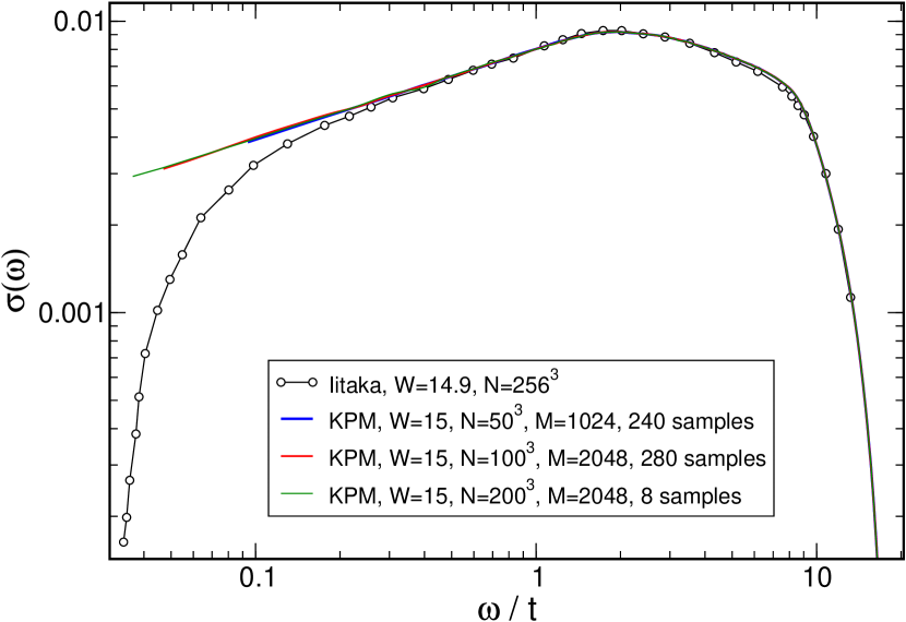
Figure 17: (Color in online edition) The optical conductivity of the Anderson model, Eq. (111), calculated with KPM and a projection method Iitaka (1998). The disorder is $W\approx 15$; temperature and chemical potential read $T=0$ and $\mu=0$.

Projection methods can also be used for the calculation of dynamical correlation functions. In this case the expansion of the density matrix, which accounts for the thermodynamics, is supplemented by a numerical time evolution. Hence, a general correlation function is written as

$$\langle A;B\rangle_{\omega}=\lim_{\epsilon\to 0}\int\limits_{0}^{\infty}\operatorname{e}^{\operatorname{i}(\omega+\operatorname{i}\epsilon)t}\operatorname{Tr}(\operatorname{e}^{\operatorname{i}Ht}A\operatorname{e}^{-\operatorname{i}Ht}BF)\,dt\,,$$ (172)

and the $\operatorname{e}^{\pm\operatorname{i}Ht}$ terms are handled by standard methods, such as Crank-Nicolson Press et al. (1986), Suzuki-Trotter de Vries and De Raedt (1993), and, very efficiently, Chebyshev expansion Dobrovitski and De Raedt (2003). Of course, not only the fermionic density matrix $F$ but also its interacting counterpart, $\exp(-\beta H)$, can be expanded in polynomials, which leads to similar methods for interacting quantum systems Iitaka and Ebisuzaki (2003).

To give an impression, in Figure 17 we compare the optical conductivity of the Anderson model calculated with KPM (see Sec. III.4.2) and with a projection approach Iitaka (1998). Over a wide frequency range the data agrees very well, but at low frequency the projection results deviate from both KPM and the analytically expected power law $\sigma(\omega)-\sigma_{0}\sim\omega^{\alpha}$. Presumably this discrepancy is due to an insufficient resolution or a too short time-integration interval. There is no fundamental reason for the projection approach to fail here.

In summary, the projection methods have a similarly broad application range as KPM, and can also compete in terms of numerical effort and computation time. For finite-temperature dynamical correlations the projection methods are characterized by a smaller memory consumption. However, in contrast to KPM they require a new simulation for each change in temperature or chemical potential, which represents their major disadvantage.

VI Conclusions & Outlook

In this review we gave a detailed introduction to the Kernel Polynomial Method, a numerical approach that on the basis of Chebyshev expansion allows for an efficient calculation of the spectral properties of large matrices and of the static and dynamic correlation functions, which depend on them. The method has a wide range of applications in different areas of physics and quantum chemistry, and we illustrated its capability with numerous examples from solid state physics, which covered such diverse topics as non-interacting electrons in disordered media, quantum spin models, or strongly correlated electron-phonon systems. Many of the considered quantities are hardly accessible with other methods, or could previously be studied only on smaller systems. Comparing with alternative numerical approaches, we demonstrated the advantages of KPM measured in terms of general applicability, speed, resource consumption, algorithmic simplicity and accuracy of the results.

Apart from further direct applications of the KPM outside the fields of solid state physics and quantum chemistry, we think that the combination of KPM with other numerical techniques will become one of the major future research directions. Certainly not only classical MC simulations and CPT, but potentially also other cluster approaches Maier et al. (2005) or quantum MC can profit from the concepts outlined in this review.

References

- Abramowitz and Stegun (1970) Abramowitz, M., and I. A. Stegun (eds.), 1970, Handbook of Mathematical Functions with formulas, graphs, and mathematical tables (Dover, New York).
- Aichhorn et al. (2003) Aichhorn, M., M. Daghofer, H. G. Evertz, and W. von der Linden, 2003, Phys. Rev. B 67, 161103.
- Alonso et al. (2001) Alonso, J. L., L. A. Fernández, F. Guinea, V. Laliena, and V. Martín-Mayor, 2001, Nucl. Phys. B 596, 587.
- Alvarez et al. (2005) Alvarez, G., C. Sen, N. Furukawa, Y. Motome, and E. Dagotto, 2005, Comp. Phys. Comm. 168, 32.
- Anderson (1958) Anderson, P. W., 1958, Phys. Rev. 109, 1492.
- Anderson and Hasegawa (1955) Anderson, P. W., and H. Hasegawa, 1955, Phys. Rev. 100, 675.
- Auerbach (1994) Auerbach, A., 1994, Interacting Electrons and Quantum Magnetism, Graduate Texts in Contemporary Physics (Springer-Verlag, Heidelberg).
- Bandyopadhyay et al. (2005) Bandyopadhyay, K., A. K. Bhattacharya, P. Biswas, and D. A. Drabold, 2005, Phys. Rev. E 71, 057701.
- Bäuml et al. (1998) Bäuml, B., G. Wellein, and H. Fehske, 1998, Phys. Rev. B 58, 3663.
- Benoit et al. (1992) Benoit, C., E. Royer, and G. Poussigue, 1992, J. Phys. Condens. Matter 4, 3125.
- Blumstein and Wheeler (1973) Blumstein, C., and J. C. Wheeler, 1973, Phys. Rev. B 8, 1764.
- Bonča et al. (1999) Bonča, J., S. A. Trugman, and I. Batistić, 1999, Phys. Rev. B 60, 1633.
- Boyd (1989) Boyd, J. P., 1989, Chebyshev and Fourier Spectral Methods, number 49 in Lecture Notes in Engineering (Springer-Verlag, Berlin).
- Chen and Guo (1999) Chen, R., and H. Guo, 1999, Comp. Phys. Comm. 119, 19.
- Cheney (1966) Cheney, E. W., 1966, Introduction to Approximation Theory (McGraw-Hill, New York).
- Coey et al. (1999) Coey, J. M. D., M. Viret, and S. von Molnár, 1999, Adv. Phys. 48, 167.
- Cullum and Willoughby (1985) Cullum, J. K., and R. A. Willoughby, 1985, Lanczos Algorithms for Large Symmetric Eigenvalue Computations, volume I & II (Birkhäuser, Boston).
- Dagotto (1994) Dagotto, E., 1994, Rev. Mod. Phys. 66, 763.
- Dagotto (2003) Dagotto, E., 2003, Nanoscale Phase Separation and Colossal Magnetoresistance: The Physics of Manganites and Related Compounds, volume 136 of Springer Series in Solid-State Sciences (Springer, Heidelberg).
- Dobrosavljević and Kotliar (1997) Dobrosavljević, V., and G. Kotliar, 1997, Phys. Rev. Lett. 78, 3943.
- Dobrosavljević and Kotliar (1998) Dobrosavljević, V., and G. Kotliar, 1998, Philos. Trans. Roy. Soc. Lond., Ser. A 356, 57.
- Dobrovitski and De Raedt (2003) Dobrovitski, V. V., and H. De Raedt, 2003, Phys. Rev. E 67, 056702.
- Drabold and Sankey (1993) Drabold, D. A., and O. F. Sankey, 1993, Phys. Rev. Lett. 70, 3631.
- Essler et al. (2005) Essler, F. H. L., H. Frahm, F. Göhmann, A. Klümper, and V. E. Korepin, 2005, The One-Dimensional Hubbard Model (Cambridge University Press, Cambridge).
- Fabricius and McCoy (1999) Fabricius, K., and B. M. McCoy, 1999, Phys. Rev. B 59, 381.
- Fehske et al. (2000) Fehske, H., C. Schindelin, A. Weiße, H. Büttner, and D. Ihle, 2000, Brazil. Jour. Phys. 30, 720.
- Fehske et al. (2004) Fehske, H., G. Wellein, G. Hager, A. Weiße, and A. R. Bishop, 2004, Phys. Rev. B 69, 165115.
- Fehske et al. (2002) Fehske, H., G. Wellein, A. P. Kampf, M. Sekania, G. Hager, A. Weiße, H. Büttner, and A. R. Bishop, 2002, in High Performance Computing in Science and Engineering, Munich 2002, edited by S. Wagner, W. Hanke, A. Bode, and F. Durst (Springer-Verlag, Heidelberg), pp. 339–350.
- Fejér (1904) Fejér, L., 1904, Math. Ann. 58, 51.
- Frigo and Johnson (2005a) Frigo, M., and S. G. Johnson, 2005a, Proceedings of the IEEE 93(2), 216, special issue on ”Program Generation, Optimization, and Platform Adaptation”.
- Frigo and Johnson (2005b) Frigo, M., and S. G. Johnson, 2005b, FFTW fast fourier transform library, URL http://www.fftw.org/.
- Furukawa and Motome (2004) Furukawa, N., and Y. Motome, 2004, J. Phys. Soc. Jpn. 73, 1482.
- Gagliano and Balseiro (1987) Gagliano, E., and C. Balseiro, 1987, Phys. Rev. Lett. 59, 2999.
- Garrett et al. (1997) Garrett, A. W., S. E. Nagler, D. Tennant, B. C. Sales, and T. Barnes, 1997, Phys. Rev. Lett. 79, 745.
- Gautschi (1968) Gautschi, W., 1968, Math. Comp. 22, 251.
- Gautschi (1970) Gautschi, W., 1970, Math. Comp. 24, 245.
- Goedecker (1999) Goedecker, S., 1999, Rev. Mod. Phys. 71, 1085.
- Goedecker and Colombo (1994) Goedecker, S., and L. Colombo, 1994, Phys. Rev. Lett. 73, 122.
- Goedecker and Teter (1995) Goedecker, S., and M. Teter, 1995, Phys. Rev. B 51, 9455.
- Gordon (1968) Gordon, R. G., 1968, J. Math. Phys. 9, 655.
- Gros and Valentí (1994) Gros, C., and R. Valentí, 1994, Ann. Phys. (Leipzig) 3, 460.
- Haydock et al. (1972) Haydock, R., V. Heine, and M. J. Kelly, 1972, J. Phys. C 5, 2845.
- Haydock et al. (1975) Haydock, R., V. Heine, and M. J. Kelly, 1975, J. Phys. C 8, 2591.
- Hohenadler et al. (2003) Hohenadler, M., M. Aichhorn, and W. von der Linden, 2003, Phys. Rev. B 68, 184304.
- Hohenadler et al. (2005) Hohenadler, M., D. Neuber, W. von der Linden, G. Wellein, J. Loos, and H. Fehske, 2005, Phys. Rev. B 71, 245111.
- Holstein (1959a) Holstein, T., 1959a, Ann. Phys. (N.Y.) 8, 325.
- Holstein (1959b) Holstein, T., 1959b, Ann. Phys. (N.Y.) 8, 343.
- Iitaka (1998) Iitaka, T., 1998, in High Performance Computing in RIKEN 1997 (Inst. Phys. Chem. Res. (RIKEN), Japan), volume 19 of RIKEN Review, pp. 136–143.
- Iitaka and Ebisuzaki (2003) Iitaka, T., and T. Ebisuzaki, 2003, Phys. Rev. Lett. 90, 047203.
- Iitaka and Ebisuzaki (2004) Iitaka, T., and T. Ebisuzaki, 2004, Phys. Rev. E 69, 057701.
- Jackson (1911) Jackson, D., 1911, Über die Genauigkeit der Annäherung stetiger Funktionen durch ganze rationale Funktionen gegebenen Grades und trigonometrische Summen gegebener Ordnung, Ph.D. thesis, Georg-August-Universität Göttingen.
- Jackson (1912) Jackson, D., 1912, Trans. Amer. Math. Soc. 13, 491.
- Jaklič and Prelovšek (1994) Jaklič, J., and P. Prelovšek, 1994, Phys. Rev. B 49, 5065.
- Jaklič and Prelovšek (2000) Jaklič, J., and P. Prelovšek, 2000, Adv. Phys. 49, 1.
- Janke (1998) Janke, W., 1998, Math. and Comput. in Simul. 47, 329.
- Jeckelmann (2002) Jeckelmann, E., 2002, Phys. Rev. B 66, 045114.
- Jeckelmann and Fehske (2006) Jeckelmann, E., and H. Fehske, 2006, in Polarons in Bulk Materials and Systems with Reduced Dimensionality, edited by G. Iadonisi, J. Ranninger, and G. D. Filippis (IOS Press, Amsterdam), volume 161 of International School of Phyics Enrico Fermi, p. ?, in press, see also http://arXiv.org/abs/cond-mat/0510637.
- Jeckelmann et al. (2000) Jeckelmann, E., F. Gebhard, and F. H. L. Essler, 2000, Phys. Rev. Lett. 85, 3910.
- Kogan and Auslender (1988) Kogan, E. M., and M. I. Auslender, 1988, Phys. Status Solidi B 147, 613.
- Korovkin (1959) Korovkin, P. P., 1959, Linejnye Operatory i teorija priblizenij (Gos. Izd. Fiziko-Matematiceskoj Literatury, Moscow).
- Kosloff (1988) Kosloff, R., 1988, J. Phys. Chem. 92, 2087.
- Kramer and Mac Kinnon (1993) Kramer, B., and A. Mac Kinnon, 1993, Rep. Prog. Phys. 56, 1469.
- Krauth (2004) Krauth, W., 2004, in New Optimization Algorithms in Physics, edited by A. K. Hartmann and H. Rieger (Wiley-VCH, Berlin), chapter 2, pp. 7–22.
- Lambin and Gaspard (1982) Lambin, P., and J.-P. Gaspard, 1982, Phys. Rev. B 26, 4356.
- Lanczos (1950) Lanczos, C., 1950, J. Res. Nat. Bur. Stand. 45, 255.
- Lanczos (1966) Lanczos, C., 1966, Discourse on Fourier series (Hafner, New York).
- Lee and Ramakrishnan (1985) Lee, P. A., and T. V. Ramakrishnan, 1985, Rev. Mod. Phys. 57, 287.
- Long et al. (2003) Long, M. W., P. Prelovšek, S. El Shawish, J. Karadamoglou, and X. Zotos, 2003, Phys. Rev. B 68, 235106.
- Lorentz (1966) Lorentz, G. G., 1966, Approximation of Functions (Holt, Rinehart and Winston, New York).
- Maier et al. (2005) Maier, T., M. Jarrell, T. Pruschke, and M. Hettler, 2005, Rev. Mod. Phys. 77, 1027.
- Mandelshtam and Taylor (1997) Mandelshtam, V. A., and H. S. Taylor, 1997, J. Chem. Phys. 107, 6756.
- Mead and Papanicolaou (1984) Mead, L. R., and N. Papanicolaou, 1984, J. Math. Phys. 25, 2404.
- Motome and Furukawa (1999) Motome, Y., and N. Furukawa, 1999, J. Phys. Soc. Jpn. 68, 3853.
- Motome and Furukawa (2000) Motome, Y., and N. Furukawa, 2000, J. Phys. Soc. Jpn. 69, 3785.
- Motome and Furukawa (2001) Motome, Y., and N. Furukawa, 2001, J. Phys. Soc. Jpn. 70, 3186, erratum.
- Neuhauser (1990) Neuhauser, D., 1990, J. Chem. Phys. 93, 2611.
- Niklasson (2003) Niklasson, A. M. N., 2003, Phys. Rev. B 68, 233104.
- Ordejón (1998) Ordejón, P., 1998, Comp. Mater. Sci. 12, 157.
- Pantelides (1978) Pantelides, S. T., 1978, Rev. Mod. Phys. 50, 797.
- Peschel et al. (1999) Peschel, I., X. Wang, M. Kaulke, and K. Hallberg (eds.), 1999, Density-Matrix Renormalization. A New Numerical Method in Physics., number 528 in Lecture Notes in Physics (Springer-Verlag, Heidelberg).
- Press et al. (1986) Press, W. H., B. P. Flannery, S. A. Teukolsky, and W. T. Vetterling, 1986, Numerical Recipes (Cambridge University Press, Cambridge).
- Rivlin (1990) Rivlin, T. J., 1990, Chebyshev polynomials: From Approximation Theory to Algebra and Number Theory, Pure and Applied Mathematics (John Wiley & Sons, New York), 2 edition.
- Robin (1997) Robin, J. M., 1997, Phys. Rev. B 56, 13634.
- Sack and Donovan (1972) Sack, R. A., and A. F. Donovan, 1972, Numer. Math. 18, 465.
- Schindelin et al. (2000) Schindelin, C., H. Fehske, H. Büttner, and D. Ihle, 2000, Phys. Rev. B 62, 12141.
- Schliemann et al. (2001) Schliemann, J., J. König, and A. H. MacDonald, 2001, Phys. Rev. B 64, 165201.
- Schollwöck (2005) Schollwöck, U., 2005, Rev. Mod. Phys. 77, 259.
- Schubert et al. (2005a) Schubert, G., A. Weiße, and H. Fehske, 2005a, Phys. Rev. B 71, 045126.
- Schubert et al. (2005b) Schubert, G., A. Weiße, G. Wellein, and H. Fehske, 2005b, in High Performance Computing in Science and Engineering, Garching 2004, edited by A. Bode and F. Durst (Springer-Verlag, Heidelberg), pp. 237–250.
- Schubert et al. (2005c) Schubert, G., G. Wellein, A. Weiße, A. Alvermann, and H. Fehske, 2005c, Phys. Rev. B 72, 104304.
- Sénéchal et al. (2000) Sénéchal, D., D. Perez, and M. Pioro-Ladrière, 2000, Phys. Rev. Lett. 84, 522.
- Sénéchal et al. (2002) Sénéchal, D., D. Perez, and D. Plouffe, 2002, Phys. Rev. B 66, 075129.
- Silver and Röder (1994) Silver, R. N., and H. Röder, 1994, Int. J. Mod. Phys. C 5, 935.
- Silver and Röder (1997) Silver, R. N., and H. Röder, 1997, Phys. Rev. E 56, 4822.
- Silver et al. (1996) Silver, R. N., H. Röder, A. F. Voter, and D. J. Kress, 1996, J. of Comp. Phys. 124, 115.
- Sirker and Klümper (2005) Sirker, J., and A. Klümper, 2005, Phys. Rev. B 71, 241101(R).
- Skilling (1988) Skilling, J., 1988, in Maximum Entropy and Bayesian Methods, edited by J. Skilling (Kluwer, Dordrecht), Fundamental Theories of Physics, pp. 455–466.
- Slevin and Ohtsuki (1999) Slevin, K., and T. Ohtsuki, 1999, Phys. Rev. Lett. 82, 382.
- Sykora et al. (2005) Sykora, S., A. Hübsch, K. W. Becker, G. Wellein, and H. Fehske, 2005, Phys. Rev. B 71, 045112.
- Tal-Ezer and Kosloff (1984) Tal-Ezer, H., and R. Kosloff, 1984, J. Chem. Phys. 81, 3967.
- Thouless (1974) Thouless, D. J., 1974, Physics Reports 13, 93.
- Turek (1988) Turek, I., 1988, J. Phys. C 21, 3251.
- Vijay et al. (2004) Vijay, A., D. J. Kouri, and D. K. Hoffman, 2004, J. Phys. Chem. A 108, 8987.
- de Vries and De Raedt (1993) de Vries, P., and H. De Raedt, 1993, Phys. Rev. B 47, 7929.
- Wang (1994) Wang, L.-W., 1994, Phys. Rev. B 49, 10154.
- Wang and Zunger (1994) Wang, L.-W., and A. Zunger, 1994, Phys. Rev. Lett. 73, 1039.
- Weiße (2004) Weiße, A., 2004, Eur. Phys. J. B 40, 125.
- Weiße et al. (1999) Weiße, A., G. Bouzerar, and H. Fehske, 1999, Eur. Phys. J. B 7, 5.
- Weiße et al. (2005) Weiße, A., H. Fehske, and D. Ihle, 2005, Physica B 359–361, 702.
- Weiße et al. (2001) Weiße, A., J. Loos, and H. Fehske, 2001, Phys. Rev. B 64, 054406.
- Wheeler (1974) Wheeler, J. C., 1974, Phys. Rev. A 9, 825.
- Wheeler and Blumstein (1972) Wheeler, J. C., and C. Blumstein, 1972, Phys. Rev. B 6, 4380.
- Wheeler et al. (1974) Wheeler, J. C., M. G. Prais, and C. Blumstein, 1974, Phys. Rev. B 10, 2429.
- Wolff (1989) Wolff, U., 1989, Phys. Rev. Lett. 62, 361.
- Zener (1951) Zener, C., 1951, Phys. Rev. 82, 403.
- Zhong et al. (1994) Zhong, Q., S. Sorella, and A. Parola, 1994, Phys. Rev. B 49, 6408.