Observation of non-exponential magnetic penetration profiles in the Meissner state — A manifestation of non-local effects in superconductors

Abstract

Implanting fully polarized low energy muons on the nanometer scale beneath the surface of a superconductor in the Meissner state enabled us to probe the evanescent magnetic field profile $B(z)$ ($0<z\lesssim 200$nm measured from the surface). All the investigated samples [Nb: $\kappa\simeq 0.7(2)$, Pb:$\kappa\simeq 0.6(1)$, Ta: $\kappa\simeq 0.5(2)$] show clear deviations from the simple exponential $B(z)$ expected in the London limit, thus revealing the non-local response of these superconductors. From a quantitative analysis within the Pippard and BCS models the London penetration depth $\lambda_{\rm L}$ is extracted. In the case of Pb also the clean limit coherence length $\xi_{0}$ is obtained. Furthermore we find that the temperature dependence of the magnetic penetration depth follows closely the two-fluid expectation $1/\lambda^{2}\propto 1-(T/T_{c})^{4}$. While $B(z)$ for Nb and Pb are rather well described within the Pippard and BCS models, for Ta this is only true to a lesser degree. We attribute this discrepancy to the fact that the superfluid density is decreased by approaching the surface on a length scale $\xi_{0}$. This effect, which is not taken self-consistently into account in the mentioned models, should be more pronounced in the lowest $\kappa$ regime consistently with our findings.

I Introduction

One of the fundamental properties of a superconductor is the Meissner-Ochsenfeld effectmeissner33 . It states that at low magnetic fields and frequencies a superconductor expels or excludes any magnetic flux from its core. However, at the surface the field penetrates on a typical length scale $\lambda$ called the magnetic penetration depth. In the London limitlondon35 , for a semi-infinite superconductor, the functional $B$ vs. $z$ dependence is an exponential one. This approximation holds for a large class of superconductors. However, as found by Pippard from a set of microwave experiments on impurity doped type-I superconductorspippard53 , this is not always true. In analogy with the anomalous skin effect Pippard introduced the concept of non-local response of the superconductor, i.e. the screening current trying to expel the magnetic field must be averaged over some spatial region of the order of $\xi$ called the coherence length. The physical interpretation of $\xi$ is, that it is the length over which the superconducting wave function can be considered as rigid, i.e. roughly speaking the size of a Cooper pair (for details see Sec. II). The non-local electrodynamical response leads to various modifications of the London theory, one being that the magnetic penetration profile $B(z)$ is no longer exponential and even changes its sign beneath the surface of the superconductor. All these findings were confirmed by the microscopic BCS theorybcs57 . Although these theoretical predictions have been known for half a century, only very recently has a “direct” measurement of the functional dependence of $B(z)$ been demonstratedsuter04a . A historical summary of the experimental work on this subject begins with that of Sommerhalder and co-workersommerhalder61a ; sommerhalder61b ; drangeid62 who showed the existence of a sign reversal of $B(z)$ by measuring the magnetic field leaking through a very thin superconducting tin film. Doezema et al.doezema84 applied magnetoabsorption resonance spectroscopy techniques to tackle the problem. The technique uses the fact that quasi-particles traveling parallel to the shielding current are bound to the surface by an effective magnetic potential. Indication of non-local effects in Al were inferred by comparing microwave induced resonant transitions between the energy levels of these bound states with transition fields calculated from the energy levels of the trapping potential, parameterized to include the shape of the non-local BCS-like potential. Due to the resonant character of the experiment, only a few specific points of the potential are probed. In addition the normal metallic state has to be understood very well in order to interpret the data. This, together with uncertainties in modeling the surface bound states, leaves room for speculations. Polarized neutron reflectometry has also been applied since specular reflectivity of neutrons spin polarized parallel or anti-parallel to $\bm{B}$ depends on the field profile. However, this technique requires model-fitting of spin-dependent scattering intensities rather than giving a direct measure of the spatial variation of the magnetic field. Up to now non-local corrections have been found to lie beyond the sensitivity of polarized neutron reflectivity techniquesnutley94 . In this paper we present magnetic field profiles measured beneath the surface of various superconductors in the Meissner state by means of low energy muon spin rotation spectroscopy (LE-$\mu$SR). The results provide a direct and quantifiable measure of non-local effects in the investigated materials (Nb, Pb, Ta) and permit the extraction of physical parameters such as the magnetic penetration depth $\lambda$ and the coherence length $\xi$. The paper is organized as follows: The next section reviews the theoretical framework necessary to understand the results and the discussion. Section III provides some information on the experimental technique including the characterization of the samples. In Sec. IV we present our data, including a discussion, followed by a summary in Sec. V.

II Theoretical Background

In this section, the theory of the response of a superconductor in respect to an external electromagnetic field will be sketched (for a rigorous derivation see Ref. schrieffer64, ). An external electromagnetic field acts on the ground state of a superconductor as a perturbation. Within standard perturbation expansion one can showschrieffer64 that the following non-local relation between the current density $\bm{j}$ and the vector potential $\nabla\wedge\bm{A}=\bm{B}$, where $\bm{B}$ is the magnetic induction, holds:

$$j_{\alpha}(\bm{r})=\sum_{\beta}\int\Big{\{}\underbrace{R_{\alpha\beta}(\bm{\rho})-\frac{e^{2}n_{\rm S}}{m^{*}}\,\delta(\bm{\rho})\delta_{\alpha\beta}}_{\displaystyle=:K_{\alpha\beta}(\bm{\rho})}\Big{\}}A_{\beta}(\bm{r}^{\prime})\,\text{d}\bm{r}^{\prime}$$ (1)

where $\bm{\rho}=\bm{r}-\bm{r}^{\prime}$, $e$ is the charge, $n_{\rm S}$ the supercurrent density, and $m^{*}$ the effective mass of the charge carrier. $K_{\alpha\beta}(\bm{\rho})$ is called the integral kernel. The vector potential $\bm{A}(\bm{r})$ needs to be properly gauged in order that Eq. (1) is physically meaningful. $R_{\alpha\beta}(\bm{\rho})$ describes the paramagnetic response, whereas the second term in the bracket reflects the diamagnetic one. If the ground state wave function of the superconductor were “rigid” with respect to all perturbations (rather than only those which lead to transverse excitations) $R_{\alpha\beta}$ would be identically zero and Eq. (1) would reduce to the second London equation

$$j_{\alpha}(\bm{r})=-\frac{1}{\mu_{0}}\,\frac{1}{\lambda_{\rm L}^{2}}\,A_{\alpha}(\bm{r})$$ (2)

with the London penetration depth $\lambda_{\rm L}=\sqrt{m^{*}/(\mu_{0}e^{2}n_{\rm S})}$, and $\mu_{0}$ the permeability of the vacuum. This, together with the Maxwell equation $\nabla\wedge\bm{B}=\mu_{0}\bm{j}$, results, for a semi-infinite sample, in the well known penetration profile

$$B(z)=B_{\text{ext}}\,\exp(-z/\lambda_{\rm L})$$ (3)

where $z$ is the depth perpendicular to the surface and $B_{\text{ext}}$ the externally applied magnetic field strength.

In situations where the paramagnetic term $R_{\alpha\beta}(\bm{\rho})$ in Eq. (1) cannot be neglected one arrives at the more complicated formula

$$B(z)=B_{\text{ext}}\,\frac{2}{\pi}\int\frac{q}{q^{2}+\mu_{0}K(q\xi,T,\ell)}\,\sin(qz)\text{d}q.$$ (4)

$K(q\xi,T,\ell)$ is the Fourier transformed kernel from Eq. (1) including the electron mean free path $\ell$. Since only the one dimensional case will be considered everything is expressed in scalar form. This equation reduces obviously to an exponential decay if $K(q\xi,T,\ell)$ is independent of $q$, and in the London limit $\mu_{0}K(q\xi,T,\ell\to\infty)=1/\lambda_{\rm L}^{2}$. Eq.(4) is valid in the case of specular reflection of the charge carriers at the surface. Another extreme limit is given by assuming diffuse scattering at the interface. A real system will not be exactly in one of the two limits. Since a quantitative analysistinkham80 shows that the difference in $\lambda$ is marginal, we use Eq.(4) for the following discussion. Still, we have verified by numerical integration of Eq.(1) that $B(z)$ for specular and diffuse scattering are closely related.

Since the electromagnetic response of the superconductor is on the length scale of $\lambda$, a local description would be sufficient if the kernel $\mu_{0}K(q\xi,T,\ell)$ is constant in the interval $0\leq q\lesssim 1/\lambda$. In the next paragraphs we will show that $\mu_{0}K(q\xi,T,\ell)$ is approximately constant for $0\leq q\lesssim 1/\xi$. From this it follows, that for $\lambda\gg\xi$ (type II) the local London limit should be quite reasonable, whereas in the opposite limit $\lambda\ll\xi$ (type I) this is not the case. For the type II case, non-local effects might play a role either in case the energy gap exhibits nodes and henceforth $\xi$ will be very anisotropickosztin97 or if $\kappa=\lambda/\xi\lesssim 1.4$. We would like to stress that the border line between the non-local and the local regime ($\kappa\approx 1.4$) does not coincide with the border line between type-I and type-II superconductivity ($\kappa=1/\sqrt{2}=0.7071\ldots$).

Knowing $K(q\xi,T,\ell)$ enables one to calculate $B(z)$. The functional dependence of $K(q\xi,T,\ell)$ was derived semi-phenomenologically by Pippard and later microscopically by Bardeen, Cooper and Schrieffer.

II.1 Pippard Kernel $K_{\rm P}(q\xi,T,\ell)$

Starting from a possible analogy between the anomalous skin effect and the Meissner-Ochsenfeld effect, Pippardpippard53 arrived at the formula for the kernel

$$\mu_{0}K_{\rm P}(q\xi,T,\ell)=\frac{1}{\lambda^{2}(T)}\,\frac{\xi_{\rm P}(T,\ell)}{\xi_{\rm P}(0,\ell)}\underbrace{\left[\frac{3}{2}\frac{1}{x^{3}}\left\{\left(1+x^{2}\right)\arctan(x)-x\right\}\right]}_{\displaystyle=g(x)},$$ (5)

with $x=q\xi_{\rm P}(T,\ell)$, and the Pippard coherence length $\xi_{\rm P}(T,\ell)$. The temperature dependence of $\xi_{\rm P}(T,\ell)$ could be explained only later by the BCS theory (see also the next section) and is

$$\frac{1}{\xi_{\rm P}(T,\ell)}=\frac{J(0,T)}{\xi_{\rm P}(0)}+\frac{1}{\ell}$$ (6)

with

$$J(0,T)=\left(\frac{\lambda(T)}{\lambda(0)}\right)^{2}\,\frac{\Delta(T)}{\Delta(0)}\,\tanh\left[\frac{\Delta(T)}{2k_{\rm B}T}\right].$$

where $\Delta(T)$ is the superconducting energy gapmuehlschlegel59 and $k_{\rm B}$ the Boltzmann constant. The weak temperature dependence of $\xi_{\rm P}(T,\ell\to\infty)$ is shown in Fig.1.

Figure 1: Temperature dependence of the Pippard coherence length $\xi_{\rm P}(T,\ell\to\infty)$ according to Eq. (6). The inset shows the temperature dependence of $J(0,T)$ within the weak coupling limit.

II.2 BCS Kernel $K_{\rm BCS}(q\xi,T,\ell)$

Starting from the weak coupling BCS modelbcs57 , one arrives at the following expression for the kernelhalbritter71

$$\mu_{0}K_{\rm BCS}(q\xi,T,\ell)=\sum_{n=0}^{\infty}\frac{1}{\Lambda_{n}(T,\ell)}\cdot g[q\xi_{n}(T,\ell)]$$ (7)

with the following set of abbreviations

$$\Lambda_{n}(T,\ell) = \frac{1}{2a}\,\lambda_{\rm L}^{2}f_{n}^{3}\left(1+\frac{\xi_{n}(T,\ell)}{\ell}\right)$$

$$\frac{1}{\xi_{n}(T,\ell)} = \frac{2}{\pi}\,\frac{f_{n}}{\xi_{0}}\,\frac{\Delta(T)}{\Delta(0)}+\frac{1}{\ell}$$ (8)

$$a = \pi\,\frac{k_{\rm B}T}{\Delta(T)},\leavevmode\nobreak\ \leavevmode\nobreak\ \xi_{0}=\frac{\hbar v_{\rm F}}{\pi\Delta(0)}$$

$$f_{n} = \sqrt{1+(2n+1)^{2}a^{2}}$$

$$\Delta(0) = \frac{\pi}{\gamma}\,k_{\rm B}T_{c}=1.764\,k_{\rm B}T_{c}.$$

The temperature dependence of $\lambda$ is defined as $1/\lambda^{2}(T):=\lim_{q\to 0}\mu_{0}K(q\xi,T,\ell)$, i.e. $\lambda(T\to 0,\ell\to\infty)=\lambda_{\rm L}$, and $\xi_{0}$ the clean limit coherence length at $T=0$. Though the BCS expression is much more involved, the $q$ dependence of the kernel is very close to the one given in the phenomenological Pippard expression Eq. (5). A comparison is given in Fig.2.

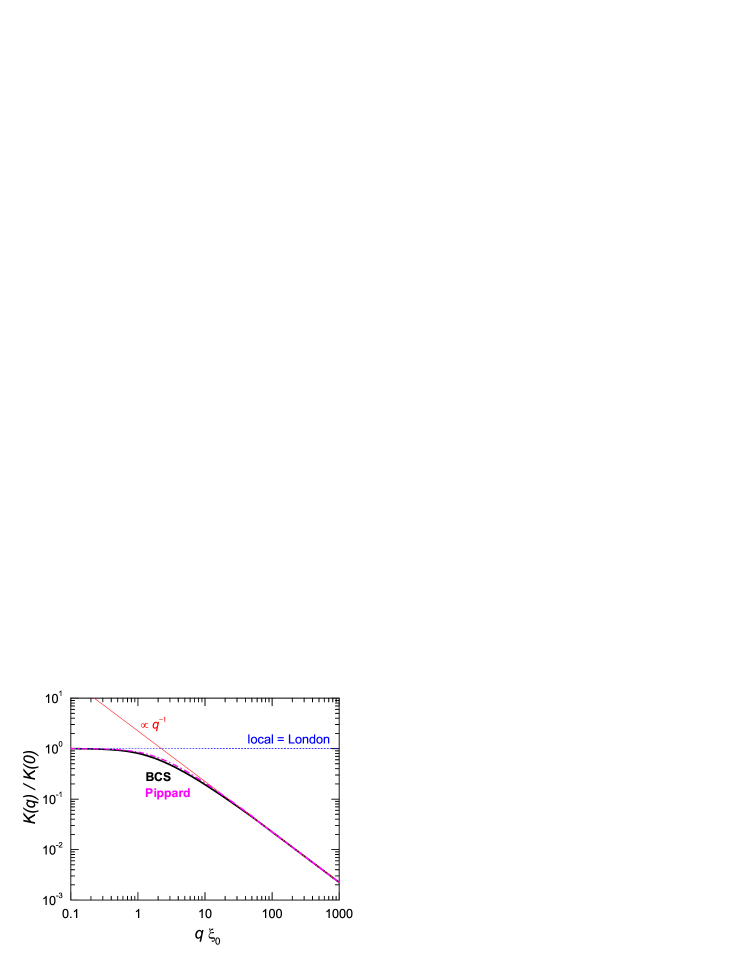
Figure 2: (Color online) $q$–dependence of the different kernels for $T\to 0$. The dashed line represents the $q$-independent London approximation. The BCS- (full) and Pippard-kernel (dash-dotted) are very similar and have a $q^{-1}$ asymptotic behavior for $q\to\infty$.

The corresponding magnetic fields can only be calculated numerically. An example of an extreme type-I superconductor, Al, is presented in Fig.3. As intuitively expected compared to the local case, the initial slope of $B(z)$ is reduced, reflecting the fact that the magnetic field penetrates deeper into the superconductor. The $\log\left|B(z)/B_{\text{ext}}\right|$ inset of Fig.3 shows initially a clear negative curvature, i.e. a deviation from the exponential behavior. The next important feature to be noticed is the sign reversal of the magnetic field before approaching zero deep inside the sample. All these findings can be made plausible by the following hand waving arguments: In the non-local case the Cooper pairs are very extended compared to the magnetic penetration profile. Since the partners within a Cooper pair do not experience the same field, the screening response is less effective and hence the slope is less steep compared to a local response. This has a second effect: since the field penetrates further beneath the surface, at some depth enough Cooper pairs will experience it and start to “overcompensate”, which accounts for the negative curvature as well as for the field reversal of $B(z)$ before approaching zero. This pictorial view is clearly an oversimplification since the screening is due to the Cooper pairs themselves, a strongly feedback coupled system, but it provides the basis for a qualitative understanding of the penetration profile.

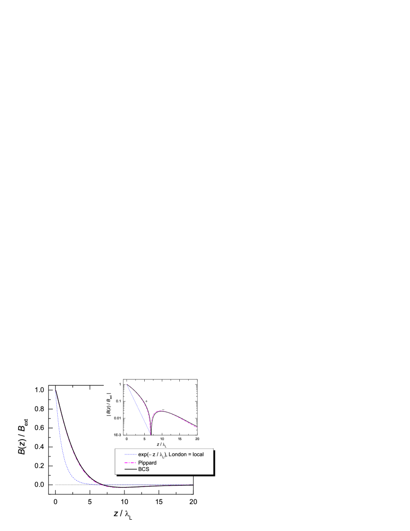
Figure 3: (Color online) The magnetic penetration profile in the Meissner state of Aluminum according to Eq.(4) for a $\xi_{0}=1600$ nm and $\lambda_{\rm L}=50$ nm. The inset shows the same curve in a log scale.

II.3 Strong Coupling Corrections

The BCS weak coupling theory assumes a weak electron-phonon interaction. This is definitely not the case for either Pb or Nb. Therefore, the much more elaborated strong-coupling theoryparks69 has to be used to calculate the properties of the superconductor. A recent review describing the strong coupling theory is found in Ref. carbotte90, . Fortunately, the outcome for the magnetic penetration profile $B(z)$ in the Meissner state is almost the same. In particular Eq.(4) still holds, and the structure of the kernel Eq.(7) is not altered, except for a renormalization of $\xi_{0}$ and $\lambda_{\rm L}$ as shown by Namnam67 . These two length scales are renormalized as

$$\lambda_{\rm L} \to \lambda_{\rm L}/\sqrt{Z}$$ (9)

$$\xi_{0} \to \xi_{0}\cdot Z$$

where the renormalization factors $Z$ for Pb, Nb and Ta are $Z_{\rm Pb}\simeq 2.55$, $Z_{\rm Nb}\simeq 2.1$, and $Z_{\rm Ta}\simeq 1.69$carbotte90 .

III Experimental Details

The samples investigated in this work were two Pb films, a Nb film, and a Ta film. The characteristic properties, relevant for the analysis are listed in Table 1.

Table 1: Characteristics of the investigated samples. $\mathrm{RRR}=[R(\mathrm{RT})-R(T_{c}+1.0)]/R(T_{c}+1.0)$

sample	$B_{\rm ext}$ (G)	thickness (nm)		$T_{c}$ (K)	RRR
		oxide layer	film
Pb-I	88.2	16(2)	430(20)	7.1(1)	16
Pb-II	89.6	5.8(3)	1055(50)	7.21(1)	23
Nb	88.2	4.2(3)	310(15)	9.24(6)	133
Ta	193.4	1.8(4)	350(15)	4.42(2)	45

The samples were sputtered directly onto a sapphire crystal using 99.999 % pure material. This permits both an excellent thermal contact to the cold finger of the cryostat and also the application of a bias to the sample, which is needed in the LE-$\mu$SR experiments to tune the implantation energy of the muons. The Pb films were sputtered at room temperature, the base pressure being $3\cdot 10^{-7}$ mbar. The Nb and Ta films were sputtered on the substrate maintained at 1000 K. The base pressure in the deposition chamber ranged between $2$ to $5\cdot 10^{-8}$ mbar. X-ray diffractometry revealed epitaxial growth of Nb with a (2 0 0) growth direction perpendicular to the substrate, and the Ta film shows a highly oriented alpha structure most probably with a (2 0 0) growth direction. The thickness of the films was determined by a high sensitivity surface profiler and Rutherford backscattering. The surface roughness of these films is given by a arithmetic mean roughness value of $<0.7$%. The critical temperature $T_{\rm c}$ was measured by means of resistivity and susceptibility measurements. The mean free path $\ell$ was estimated according to our resistivity data.

The oxide layers of Nb and Ta are extremely stable as discussed extensively in Ref.halbritter87, . The dieletric $\mathrm{Nb_{2}O_{5}}$ forms at the surface of Nb and acts as a very good protection layer. The typical $\mathrm{Nb_{2}O_{5}}$ layer thickness found under the described growing conditions is $\simeq 5$ nm. Ta forms a $\mathrm{Ta_{2}O_{5}}$ oxide layer with a typical saturation thickness of $\simeq 2$ nm, which again acts as a very well protection layer for the Ta film. The thickness of the oxide layer as determined by our measurements is in excellent agreement with the findings in the literature.

The LE-$\mu$SR method makes use of the muon spin rotation techniqueschenck85 ($\mu$SR) where $\sim 100$% polarized positive muons ($\mu^{+}$) implanted in a solid sample rapidly thermalize ($\sim 10$ ps) without noticeable polarization loss. The spin evolution of the ensemble after the implantation is then measured as a function of time. The evolution can be monitored by using the fact that the parity violating muon decay is highly anisotropic with the easily detectable positron emitted preferentially in the direction of the $\mu^{+}$ spin at the moment of the decay.

Counting the variation of the decay positron intensity $N(t)$ with one or more detectors as a function of time after the muon has stopped in the sample, it is possible to determine $P(t)$, the time dependence of the polarization along the initial muon spin direction.

The experimentally obtained time histograms have the form

$$N(t)=N_{0}\,\left[1+A_{0}\,\frac{P(t)}{P(0)}\right]\,e^{-t/\tau_{\mu}}.$$ (10)

$N_{0}$ is a normalization constant reflecting the total number of muons recorded. The exponential describes the decay of the $\mu^{+}$ and $A_{0}$ is the maximum observable asymmetry of the decay (theoretically $1/3$ in case of 100% polarization and when integrating over all positron energies). The relevant information about the system under consideration is contained in the term $A_{0}\,P(t)/P(0)$.

Unlike conventional $\mu$SR techniques which make use of the energetic muons ($\sim 4$ MeV) originating from $\pi^{+}$ decay at rest (“surface” muons), LE-$\mu$SR makes use of epithermal muons ($\sim 15$ eV) extracted after moderation of surface muons from a thin film of a weakly bound van der Waals cryosolid (wide band gap insulator)morenzoni94 ; morenzoni00 . By re-accelerating the epithermal muons up to 20 keV and biasing the sample, it is possible to tune the implantation energy in the range of 0.5 to 30 keV and thus to implant the muons beneath the surface of any material in a range of up to about 300 nm and a spatial resolution down to 1 nm. Details concerning the $\mu^{+}$ stopping distribution will be given in Sec.IV.

The measurements were carried out as follows: A magnetic induction $B_{\rm ext}$ parallel to the sample surface was applied after zero field cooling the sample. The incident muon spin was parallel to the surface and perpendicular to $B_{\rm ext}$.

IV Results and Analysis

Figure 4: Typical time spectra $A_{0}\,P(t,E)/P(0,E)$. The shown data are from sample Pb-II, zero field cooled, $T=3.05$ K, $B_{\rm ext}=8.82(6)$ mT. Top: $\mu^{+}$ implantation energy $E=5.2$ keV. Bottom: $E=14.8$ keV.

The applied magnetic field was determined from the Larmor precession frequency of the muon spin at $T>T_{c}$. In this case the measured polarization simply exhibits the undamped precession of the muon spin ensemble $P(t)\propto\cos(\gamma_{\mu}B_{\rm ext}t+\phi)$. In the Meissner state ($T<T_{c}$), the $\mu^{+}$ ensemble, stopping in the surface layer, is sampling $B(z)$, thus the muons will precess in various fields, depending on where they actually stop (distance to the interface). This yields a damped $P(t)$, reflecting the spatial distribution of the magnetic field close to the surface. Fig.4 shows some typical time spectra according to Eq.(10). From these spectra, the magnetic field distribution $p(B,E)$ is obtained by Fourier transform

$$p(B,E)=\frac{2}{\sqrt{2\pi}}\int_{0}^{\infty}A_{0}\,\frac{P(t,E)}{P(0,E)}\,\cos(\gamma_{\mu}Bt+\phi)\,\text{d}t$$ (11)

where $\gamma_{\mu}$ is the gyromagnetic ratio of the $\mu^{+}$ and $\phi$ an angle taking into account the concrete detector geometry. $E$ is the implantation energy of the muons. To obtain $p(B,E)$ we used a maximum entropy algorithm, which proved to be much more robust than the usual Fourier transform methods, especially in the case of limited available statisticswu97 ; skilling84 ; rainford94 ; riseman00b .

To determine $B(z)$ knowledge of the muon stopping distribution $n(z,E)$ is needed. The situation is similar to the case of magnetic resonance imaging where a measured nuclear resonance frequency has to be translated into a space coordinate. We use the Monte Carlo code TRIM.SPeckstein91 whose reliability to predict implantation profiles of low energy $\mu^{+}$ in various materials has been confirmed by experimental testingmorenzoni02 . The functional relation between $n(z,E)$ and $p(B,E)$ is

$$n(z,E)\,\text{d}z=p(B,E)\,\text{d}B$$ (12)

which states nothing else than the probability that a given implanted muon with incident energy $E$ stopping in the interval $[z,z+\text{d}z]$, will experience a field in the interval $[B,B+\text{d}B]$ with the probability $p(B,E)$ [assuming a monotonous $B(z)$]. Integrating Eq.(12) on both sides yields

$$\int_{0}^{z}n(\zeta,E)\,\text{d}\zeta=\int_{B(z)}^{\infty}p(\beta,E)\,\text{d}\beta$$ (13)

which is, for a chosen $z$, an equation for $B$. Since $n(z,E)$ can be calculated and $p(B,E)$ can be measured by means of LE-$\mu$SR, the magnetic field penetration profile can be determined. Fig.5 shows an example of a $B(z)$ determination.

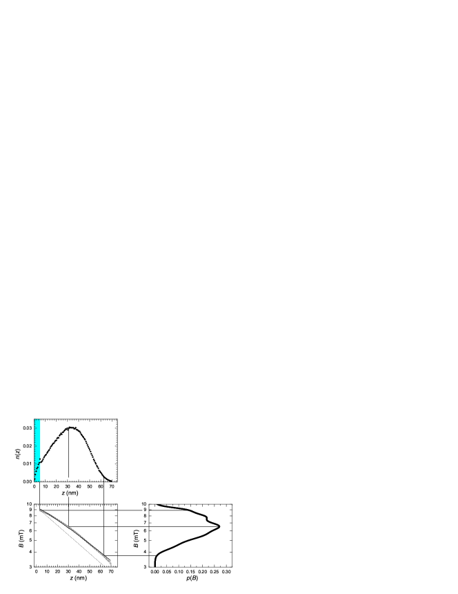
Figure 5: (Color online) Magnetic penetration profile $B(z)$ in sample Pb-II at $T=3.03$ K. The $\mu^{+}$ implantation energy was $E=5.2$ keV. Top graph: $\mu^{+}$ stopping profile $n(z,E)$ from the Monte Carlo code TRIM.SP. Bottom right graph: $p(B,E)$ maximum entropy analysis of $A_{0}\,P(t)/P(0)$ [see Eq.(10)]. Bottom left graph: $B(z)$ field determination according to Eq.(13). The solid line in $B(z)$ is the best fit for the BCS kernel [Eqs.(4), (7)], whereas the dashed line shows the London limit for parameters obtained from the BCS fit. The shaded area of $n(z,E)$ shows the Pb oxide layer.

With this approach it is possible to determine the whole $B(z)$ functional dependence from a single measurement at one specific implantation energy. Still, we determined $B(z)$ at various energies which results in a set of overlapping curves. This self-consistence check further demonstrates the reliability of the Monte Carlo code used to determine $n(z,E)$. For a further crosscheck we used an additional approach to determine $B(z)$, which allows a more rigorous statistical error estimate. With a very narrow stopping distribution, the following two approaches also lead to a $B(z)$: (i) Plotting the spatial coordinate $z_{p}$ for which the stopping distribution $n(z,E)$ is maximal (peak value), against the field value $B_{p}$ where the field distribution $p(B,E)$ has its maximum, a $B_{p}(z_{p})=B(z)$ results for a set of different implantation energies $E$. (ii) Instead of choosing the peak position, the mean values $\langle z\rangle=\int z\,n(z,E)\,\text{d}z$ and $\langle B\rangle=\int B\,p(B,E)\,\text{d}B$ can be used which again leads to $\langle B\rangle$ vs. $\langle z\rangle=B(z)$ for a set of different $E$. However, it has to be taken into account that the stopping distribution $n(z,E)$ is not very narrow and therefore a more elaborate calculation is needed. The details of such an analysis are given in Appendix A. The results can be summarized as follows: Both approaches introduce minor systematic errors. The systematic error of the peak value approach could mimic deviations of an exponential decay reminiscent of non-local effects $\{$negative initial curvature of $\log[B(z)]\}$ and therefore this approach was excluded. The mean value determination is the appropriate choice, since this method only produces systematic errors opposing possible non-local effects, i.e. an exponential decaying magnetic field profile is slightly deformed so that $\log[B(z)]$ has a positive initial curvature. The determination based on mean values could, in the worst case, only lead to an underestimation of present non-local effects or even wash them out.

The mean values $\langle z\rangle$ were determined directly from the Monte Carlo stopping distribution. The asymmetries, measured at various implantation energies, were fitted within a Gaussian relaxation model to

$$A_{0}\,\frac{P(t)}{P(0)} = A_{\rm BG}^{\rm tot}\;\exp\left[-\frac{1}{2}\;(\sigma_{\rm BG}t)^{2}\right]\cos(\gamma_{\mu}B_{\rm ext}t+\phi)+$$ (14)

$$+A_{\rm SC}\;\exp\left[-\frac{1}{2}\;(\sigma_{\rm SC}t)^{2}\right]\cos(\gamma_{\mu}B_{\rm SC}t+\phi)-$$

$$-A_{\rm BS}.$$

$\phi$ is a phase describing the relative position of the positron detectors. The observable asymmetry $A_{0}$ is modeled by 3 contributions $A_{0}=A_{\rm SC}+A_{\rm BG}^{\rm tot}+A_{\rm BS}$. For our present experimental setup $A_{0}=0.27$. $A_{\rm SC}/A_{0}$ gives the weight of the muons stopping in the superconductor. $A_{\rm BG}^{\rm tot}/A_{0}$ is the portion of muons either stopping in the oxide layer or in the sample surrounding. These muons experience the external field $B_{\rm ext}$. $A_{\rm BS}/A_{0}$ is the portion of backscattered muons. The backscattered muons form muoniummorenzoni02 (a hydrogen like electron-muon bound state with a gyromagnetic ratio $\gamma_{\rm Mu}\simeq 103\gamma_{\mu}$). Due to its large $\gamma_{\rm Mu}$, muonium has a much higher precession frequency compared to $\mu^{+}$ which results, in the present experiment, in an instant depolarization (extremely short dephasing time, filtering due to sampling of the time signal). This leads to an effective reduction in the observable asymmetry as written in Eq.(14). The various weights of the asymmetries were fixed according to the Monte Carlo simulation of $n(z,E)$. Therefore the only free fitting parameters are $B_{\rm SC}$, which corresponds to $\langle B\rangle$ in this Gaussian relaxation model approximation, and the two depolarization rates $\sigma_{\rm BG}$, and $\sigma_{\rm SC}$. Fig.6 shows a typical result together with two $B(z)$ profiles determined from Eq.(13) for different implantation energies. We would like to stress that the mean value approach to determining $B(z)$, due to slight systematic errors, rather underestimates the deviation from an exponential magnetic penetration profile. Still, deviations from the exponential behavior of $B(z)$ are clearly present, thus confirming the non-local response.

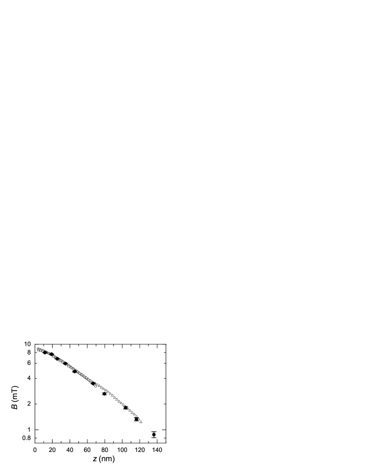
Figure 6: Mean value determination of $B(z)$ (solid dots) in sample Pb-II at $T=3.03$ K, together with integral approach [Eq.(13)] for $E=5.2$ keV (open circles) and $E=14.8$ keV (open triangles).

Additional evidence about the power to detect small variations of the magnetic penetration profile is given by the previously measured $B(z)$ data of the high temperature superconductor $\mathrm{YBa_{2}Cu_{3}O_{7-\delta}}$ (optimally doped; for details see Ref.jackson00b, ). In this clear cut type II superconductor [$\xi_{0}\approx 1.5$ nm, $\lambda_{\rm L}=146(3)$ nm] a perfect exponential $B(z)$ is expected, at least for temperatures $\gtrsim 1$ K. Below $T\lesssim 1$ K there might be deviations from the exponential behavior due to the d-wave pairing character in this compound which can lead to substantial non-linear and non-local effectsyip92 ; kosztin97 ; amin98 . We reanalyzed these data according to the above discussion. The results for $T=20$ K are shown in Fig.7, which clearly demonstrates the exponential form of $B(z)$.

Figure 7: Magnetic penetration profile $B(z)$ of the high temperature superconductor $\mathrm{YBa_{2}Cu_{3}O_{7-\delta}}$ at $T=20$ K ($T_{c}=87.5$ K). The $B(z)$ obtained from the mean values is displayed by solid circles whereas the other points show the integral determined field profile based on Eq.(13).

After having established the reliability of our approach to determine $B(z)$, we turn to the discussion of the data. Fig.8 shows a collection of our results for Pb; Fig.10 shows the Nb and Fig.11 the Ta data. The low temperature data of both Pb samples show a clear deviation from an exponential decay law, indubitable evidence for the presence of non-local effects. Furthermore, increasing the temperature leads to less-pronounced curvature as expected, since very close to $T_{c}$ non-local effects should disappear altogether (strong temperature dependence of $\lambda$ for $T\to T_{c}$; weak one of $\xi$ [see Fig.1]). Unfortunately, the range where a sign reversal of $B(z)$, predicted by theory, should appear, is experimentally not accessible yet. To compare with theory, the data were fitted according to Eq.(4) for the Pippard kernel [Eq.(5)] and the BCS kernel [Eqs.(7),(II.2)], respectively. Since the temperature dependence of $\lambda$ is undefined within the Pippard model, we chose the two-fluid approximation $\lambda(t)=\lambda_{0}/\sqrt{1-t^{4}}$, with $t=T/T_{c}$. $\lambda_{0}$ is an effective London penetration depth, taking into account corrections due to the scattering of electrons. In the clean limit ($\ell\to\infty$) $\lambda_{0}=\lambda_{\rm L}$. The temperature dependence of $\lambda$ within the BCS model is given implicitly by the Eqs.(7),(II.2), where again $\lambda_{0}$ is used to indicate an effective London penetration depth. The fits to the data are shown in Fig.8 and were obtained in the following way: for the low-temperature high-statistic data it was possible to fit $\lambda_{0}$ and $\xi_{0}$. For the rest of the data, $\xi_{0}$ was fixed to the value found at low temperature. This was necessary, since by approaching $T_{c}$, the magnetic penetration profile becomes more and more exponential due to the strong temperature dependence of $\lambda$. As a consequence, the $\xi$-dependence of $B(z)$ weakens resulting in a drastically growing uncertainty to determine the parameter.

In the models used to analyze $B(z)$ a temperature dependence of the magnetic penetration $\lambda(T)$ is assumed (Pippard Sec.II.1) or implicitly given (BCS Sec.II.2). If these models describe the temperature dependence of $\lambda(T)$ correctly, $\lambda_{0}$ should be a constant value within the error bars for all the data sets. Fig.9 shows a graph where $\lambda_{0}$ is plotted versus the reduced temperature $t=T/T_{c}$ for both models. For the two-fluid temperature dependence, assumed in our Pippard model, $\lambda_{0}$ is indeed temperature independent, except for data close to $T_{c}$. The weak coupling BCS temperature dependence for the magnetic penetration length, however, produces a clear temperature dependent $\lambda_{0}$ meaning that the real temperature dependence of the energy gap $\Delta(T)$ does not follow exactly the weak coupling prediction. Table 2 shows the collected results.

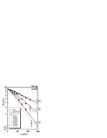
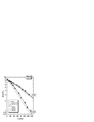
Figure 8: (Color online) Magnetic penetration profiles for Pb at various temperatures. Left graph: Data from sample Pb-I. Right graph: Data from sample Pb-II. The solid lines are BCS fits to the data, whereas the dashed line represents $B(z)=B_{\rm ext}\exp(-z/\lambda)$, where the $\lambda$ from the BCS fit is used.

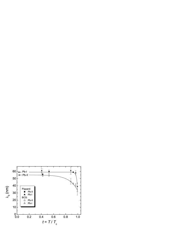
Figure 9: $\lambda_{0}$ determined at various temperatures $t=T/T_{c}$ for the Pb data. The temperature dependence of $\lambda$ in the Pippard model was chosen as $1/\lambda^{2}\propto\sqrt{1-t^{4}}$, whereas in the BCS model the temperature dependence is given implicitly by Eqs.(4),(7),(II.2). The curves are guides to the eyes.

In the case of Nb (Fig.10) the limited statistics of the data do not allow us to fit $\xi_{0}$ directly. For the analysis it was therefore fixed to its literature value (see Table 2). This system is at the borderline between the non-local and local regimes. Therefore $B(z)$ was also analyzed with a simple exponential model, leading to $\lambda_{0}^{\rm exp}=33(3)$ (nm) which is similar to the non-local value given in Table 2. The $\chi^{2}$ suggests that also for Nb the non-local regime is the appropriate one, but definitely higher quality data are needed to resolve this issue.

The Ta data (Fig.11) show a more pronounced deviation from an exponential decay law. As for Nb it was necessary in this case to fix $\xi_{0}$ to the literature value. Table 2 summarizes the results. In the data analysis we also considered the possibility of spurious effects related to surface roughness or thickness variation of the film due to the presence of terrace-like structures. If these structures have a lateral size smaller or comparable to the coherence length, the screening current will be very ineffective, thus resulting in a dead layer at the surface. We effectively find a better fit to the data assuming the presence of such a dead layer (see Fig.12 and Table 2) in addition to the previously mentioned oxide layer. The other case of surface terraces with lateral extension $\gg$ $\xi_{0}$ would mimic a thickness distribution of the film. Numerical simulations have shown that such a thickness variation would only marginally affect the magnetic penetration depth. A closer look at the Ta curves shows that compared to the other systems the fit based on the BCS or Pippard model does reproduce the data in a less satisfactory way. One possible origin for this discrepancy is the neglect in both models of the suppression of the supercurrent density on approaching the surface. Fig.12 sketches the situation. The models discussed in Sec.II assume $n_{\rm S}$ to be constant up to the surface (dashed line). However, from the Ginzburg-Landau theory it is known (see e.g. Ref.poole95, ) that close to the surface the order parameter, and hence $n_{\rm S}$, are reduced. Such a reduction in $n_{\rm S}$ makes the screening less effective, which, on top of the non-local effects, would lead to a more pronounced deviation from the exponential penetration profile than estimated by Eq.(4) or its diffuse scattering counterpart. In the presently investigated samples we expect such an effect to be more pronounced in the cleaner superconducting Ta than in Pb (where also small deviations from the theoretical curves are possibly present in Fig.8) because of its lower effective $\kappa$. In order to quantify these effects in a comparison with our experimental findings, it would be very useful to have a self-consistent theoretical description of the physics outlined above.

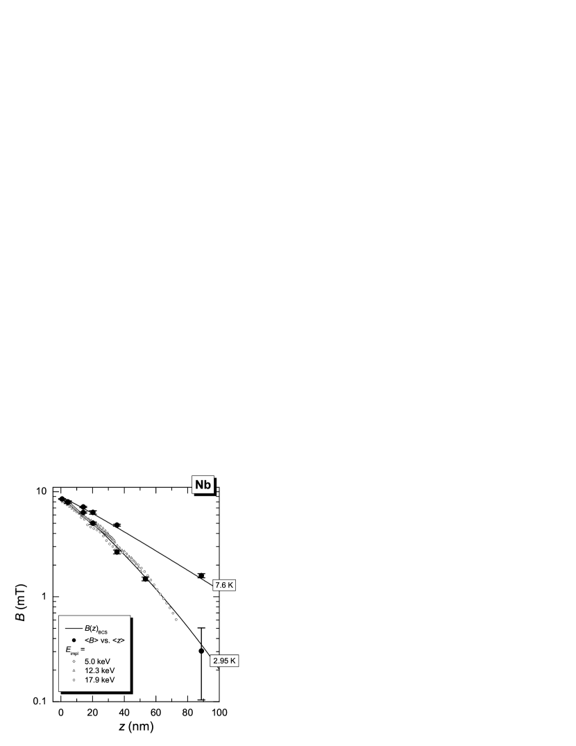
Figure 10: Mean value determination (solid dots) in Nb at $T=2.95$ K and $T=7.6$ K, together with the integral approach. The solid lines show BCS fits.

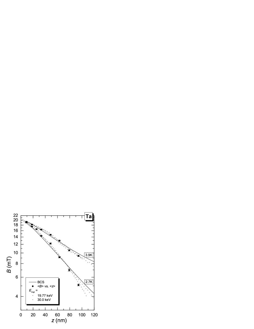
Figure 11: Magnetic penetration profiles for Ta at various temperatures. The solid lines show BCS fits.

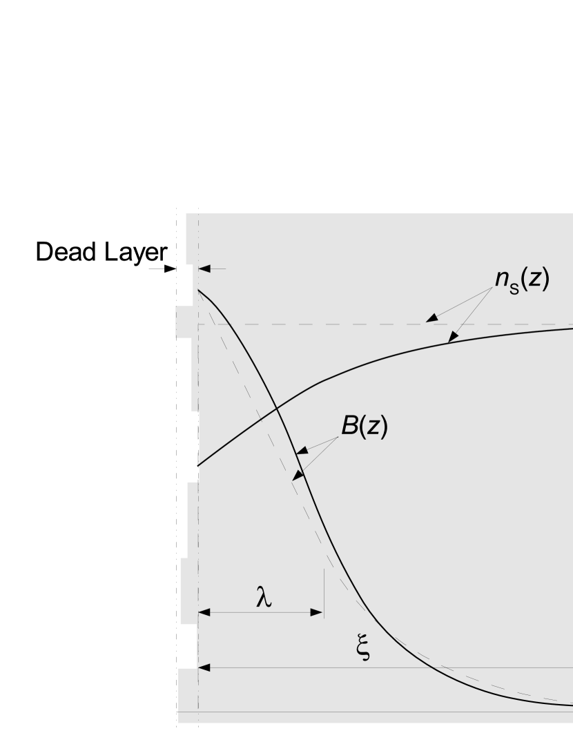
Figure 12: Effect on $B(z)$ of the suppression of $n_{\rm S}(z)$ at the surface. The shaded area represent the sample cross-section. The left side shows a surface with a terraces of typical size $\lesssim\xi_{0}$, which results in a “dead layer”. The dashed lines show ideal superfluid density $n_{\rm S}(z)$ and magnetic penetration profile $B(z)$, respectively. The solid lines are the corresponding more realistic ones.

Table 2: Results of the analysis for Pb, Nb and Ta. The values for $\lambda_{0}^{\rm BCS,P}$ given, are the low temperature values. The “dead layer” corresponds to a shift of the $z$-origin of $B(z)$.

sample	compound	$\lambda_{0}^{\rm BCS,P}$	$\xi_{0}$	dead layer
		(nm)	(nm)	(nm)
Pb-I	Pb	59(3)	90(5)	6(1)
Pb-II	Pb	55(1)	90(5)	3(2)
Nb	Nb	27(3)	39(fixed)poole95	2(2)
Ta	Ta	52(2)	92(fixed)poole95	3(1)

V Summary

We have performed low energy muon spin rotation spectroscopy experiments (LE-$\mu$SR) on Pb, Nb and Ta films in the Meissner state. The magnetic penetration profile $B(z)$ into the superconductor has been determined on the nano-meter scale, thus providing a model independent measure of the Meissner screening profile. $B(z)$ shows clear deviations from the simple exponential decay law as expected in the Pippard regime where the relation between the current density and the vector potential is non-local in nature. Analyzing the data within the Pippard and BCS model, the coherence length $\xi_{0}$ and the London penetration length $\lambda_{\rm L}$ could be deduced. Furthermore we could show that the two-fluid model approximation for the temperature dependence of $\lambda\propto 1/\sqrt{1-(T/T_{c})^{4}}$ is closer to the experiment than the BCS one which is $\lambda\propto 1/\sqrt{K_{\rm BCS}(q\to 0,T,\ell\to\infty)}$. These experiments based on the local profiling of the magnetic field penetrating at the surface are the first measurements showing the non-local nature of superconductivity in Pb, Nb and Ta on the nanometer scale, and verify directly and quantitatively the longstanding predictions of Pippard. $B(z)$ for Ta deviates substantially from the simplest theoretical approach, which we attribute to the neglect of the reduced superfluid density on approaching the surface.

Appendix A Modeling the determination of the magnetic field profile

Figure 13: Model stopping distribution $n(z,E)$ of low energy muons.

As pointed out in the paper the integral determination of $B(z)$ [Eq.(13)] is the most effective method since it is able to generate a complete curve from a single implantation energy. As a cross-check of the use of the maximum entropy method to determine $p(B,E)$ and $B(z)$ via Eq.(13), where the determination of the statistical error is an unresolved issue, we analyzed the $\mu$SR data directly in the time domain which permits estimation of the statistical errors. The time domain modeling used in our analysis has the disadvantage of introducing systematic errors and only one of the discussed approaches is acceptable for the investigation of non-local effects.

Two sets of models, which will be discussed separately in the following paragraphs, can be treated analytically. The resulting trend is similar in both cases, meaning that the “mean value determination” (Sec.A.1) slightly overestimates the real $B(z)$, whereas the “peak value determination” (Sec.A.2) always slightly underestimates $B(z)$. In the situation where one is looking for non-local effects, characterized by an initial negative curvature of $\log\left|B(z)/B_{\text{ext}}\right|$, the mean value reconstruction is the method of choice because only it can produce systematic errors with a positive curvature, and henceforth, in the worst case, can only hide the presence of a negative curvature. All these results are compiled in Fig.14.

A.1 Mean Value Determination of $B(z)$

The muon stopping distribution can only be calculated by Monte Carlo codes. For the following discussion a simple stopping distribution mimicking a realistic one is needed. We take as a model stopping distribution $n(z,E)$

$$n(z,E)=n_{0}\,(z_{0}-z)\,z^{4},\leavevmode\nobreak\ \leavevmode\nobreak\ \leavevmode\nobreak\ z\in[0,z_{0}],$$ (15)

where $n_{0}=30\,z_{0}^{-6}$ is the normalization factor and $z_{0}$ the maximum distance, which an implanted muon can reach. This function is an acceptable approximation for a realistic implantation profile (Fig.13).

The mean value of $z$ is

$$\langle z\rangle=\frac{5}{7}\,z_{0}.$$ (16)

Assuming further

$$B(z)=B_{\rm ext}\exp(-z/\lambda)$$ (17)

one gets, utilizing the identity $n(z,E)\,\text{d}z=p(B,E)\,\text{d}B$,

$$\langle B\rangle = \int_{0}^{z_{0}}\text{d}z\,B(z)n(z,E)$$

$$= B_{\rm ext}\,n_{0}\lambda^{2}\left[24\lambda^{3}(z_{0}-5\lambda)+e^{-z_{0}/\lambda}\left\{z_{0}^{4}+8\lambda z_{0}^{3}+36\lambda^{2}z_{0}^{2}+96\lambda^{3}z_{0}+120\lambda^{4}\right\}\right]$$

$$= B_{\rm ext}\exp(-\langle z\rangle/\lambda)+f(\langle z\rangle),\leavevmode\nobreak\ \leavevmode\nobreak\ \leavevmode\nobreak\ \leavevmode\nobreak\ \leavevmode\nobreak\ f(\langle z\rangle)\geq 0$$

with $\lim\limits_{\langle z\rangle\to 0}f(\langle z\rangle)=0$ and $f(\langle z\rangle)<\langle B\rangle(\langle z\rangle)$ in the first two decades as shown in Fig.14. Notice that the curvature of $f(\langle z\rangle)$ is positive.

In order to have an estimate not only for an exponential $B(z)$, also the following $B(z)$ (resembling a non-local field profile close to the solution in the extreme anomalous limittinkham80 $\xi\gg\lambda$) was analyzed

$$B(z)=B_{\rm ext}\,\exp\left(-\frac{\sqrt{3}}{2}\,Qz\right)\,\cos\left(\frac{1}{2}\,Qz\right),$$ (19)

where $Q=\left[\displaystyle\frac{\displaystyle 3\pi}{\displaystyle 4}\,\displaystyle\frac{\displaystyle 1}{\displaystyle\lambda_{\rm L}^{2}\xi_{0}}\right]^{1/3}$. Also here an exact solution for the mean value can be given

$$\langle B\rangle/B_{\rm ext} = c_{0}+c_{1}\exp\left(-\frac{7\sqrt{3}}{10}\,Q\langle z\rangle\right)\,\cos\left(\frac{7}{10}\,Q\langle z\rangle\right)+$$ (20)

$$+c_{2}\exp\left(-\frac{7\sqrt{3}}{10}\,Q\langle z\rangle\right)\,\sin\left(\frac{7}{10}\,Q\langle z\rangle\right)$$

where the coefficients $c_{i}$ are

$$c_{0} = -\frac{1125000\,(7\sqrt{3}\,Q\langle z\rangle-50)}{117649\,(Q\langle z\rangle)^{6}}$$

$$c_{1} = -\frac{375\,\left[150000+84000\,\sqrt{3}\,Q\langle z\rangle+44100\,(Q\langle z\rangle)^{2}-2401\,(Q\langle z\rangle)^{4}\right]}{117649\,(Q\langle z\rangle)^{6}}$$

$$c_{2} = -\frac{375\,\left[12000+6300\sqrt{3}\,Q\langle z\rangle+3920\,(Q\langle z\rangle)^{2}+343\sqrt{3}(Q\langle z\rangle)^{3}\right]}{16807\,(Q\langle z\rangle)^{5}}.$$

These formulae look rather ugly but as can be seen in Fig.14, the result is very similar to the simpler case discussed before.

A.2 Peak Value Determination of $B(z)$

First lets assume the model stopping distribution from Eq.(15). The peak value of the spatial coordinate is

$$z_{p}=\frac{4}{5}\,z_{0}.$$ (21)

The corresponding peak position is obtained from

$$p(B,E) = n(z,E)\,\left|\frac{dB}{dz}\right|^{-1}$$

$$= \frac{\lambda}{B}\,(\lambda\,\ln(B_{\rm ext}/B))^{4}\,\left(z_{0}-\lambda\,\ln(B_{\rm ext}/B)\right),$$

with $B\in[B_{\rm ext}e^{-z_{0}/\lambda},B_{\rm ext}]$. Since we are only interested in the peak position, the normalization factor was suppressed. It follows that

$$B_{p} = B_{\rm ext}\exp\left[\frac{-1}{2\lambda}\left(z_{0}-5\lambda+\sqrt{(z_{0}+5\lambda)^{2}-4z_{0}}\right)\right]$$ (22)

$$= B_{\rm ext}\exp(-z_{p}/\lambda)-g(z_{p}),$$

with $g(z_{p})\geq 0$ and $\lim_{z_{p}\to 0}g(z_{p})=0$. The results found so far are compiled in Fig.14.

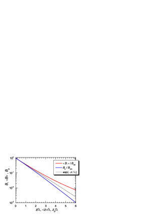
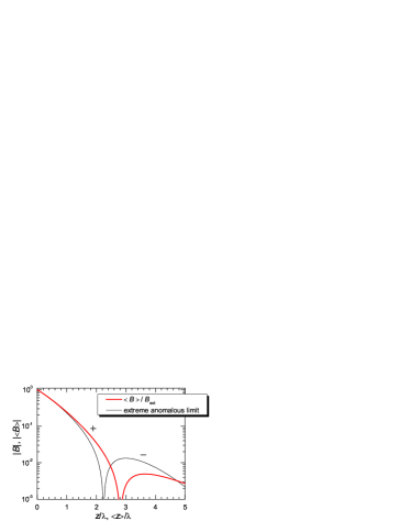
Figure 14: (Color online) Left: Analytic results for mean- and peak value determination assuming an exponential $B(z)$.
Right: Extreme anomalous limit result for the mean value determination of $B(z)$.

Another ansatz, which is extremely close to the our analysis is the following: Instead of assuming a model distribution $n(z,E)$ [Eq.(15)], one assumes that $p(B,E)$ is Gaussian, i.e. the time dependent LE-$\mu$SR signal is Gaussian damped.

$$p(B,E)=\frac{1}{\sqrt{2\pi}\delta B}\,\exp\left[-\frac{1}{2}\,\left(\frac{B-B_{0}}{\delta B}\right)^{2}\right].$$ (23)

with $B_{0}$ the position of the Gaussian peak. $\delta B$ is the width of the distribution. Assuming furthermore an exponential $B(z)$ [Eq.(17)], one arrives at the following stopping distribution

$$n(z,E)=\frac{1}{\sqrt{2\pi}\lambda}\,\frac{B_{0}}{\delta B}\exp\left[-\frac{1}{2}\,\left(\frac{B_{\rm ext}e^{-z/\lambda}-B_{0}}{\delta B}\right)^{2}-\frac{z}{\lambda}\right]$$ (24)

The peak values are than given by

$$B_{p} = B_{0}$$

$$n_{p} = \lambda\,\ln\left[\frac{B_{\rm ext}}{2\delta B^{2}}\left(\sqrt{B_{0}^{2}+4\delta B}-B_{0}\right)\right],$$

which leads to

$$B_{p}(z_{p})=B_{\rm ext}\,e^{-z_{p}/\lambda}\left[1-\left(\frac{\delta B}{B_{\rm ext}}\right)^{2}e^{+2z_{p}/\lambda}\right],$$ (25)

showing the same trend as in the previously discussed case.

In conclusion, one finds that the peak value approach to determine $B(z)$ leads to systematic errors that can mimic a magnetic penetration profile of a non-local superconductor and therefore has to be excluded from such an analysis. The mean value determination of $B(z)$ also introduces systematic errors, however they tend to diminish real non-local effects and are therefore less dangerous.

References

- (1) W. Meissner and R. Ochsenfeld, Die Naturwissenschaften 21, 787 (1933).
- (2) F. London and H. London, Proc. R. Soc. London, Ser. A 149, 71 (1935).
- (3) A. B. Pippard, Proc. Roy. Soc. (London) A216, 547 (1953).
- (4) J. Bardeen, L. N. Cooper, and J. R. Schrieffer, Phys. Rev. 108, 1175 (1957).
- (5) A. Suter, E. Morenzoni, R. Khasanov, H. Luetkens, T. Prokscha, and N. Garifianov, Phys. Rev. Lett. 92, 087001 (2004).
- (6) R. Sommerhalder and H. Thomas, Helv. Phys. Acta 34, 29 (1961).
- (7) R. Sommerhalder and H. Thomas, Helv. Phys. Acta 34, 265 (1961).
- (8) K. E. Drangeid and R. Sommerhalder, Phys. Rev. Lett. 8, 467 (1962).
- (9) R. E. Doezema, J. N. Huffaker, S. Whitmore, J. Slinkman, and W. E. Lawrence, Phys. Rev. Lett. 53, 714 (1984).
- (10) M. P. Nutley, A. T. Boothroyd, C. R. Staddon, D. M. Paul, and J. Penfold, Phys. Rev. B 49, 15789 (1994).
- (11) J. R. Schrieffer, Theory of Superconductivity (Addison Wesley, San Francisco, 1964).
- (12) M. Tinkham, Introduction to Superconductivity (Krieger, New York, 1980).
- (13) I. Kosztin and A. J. Leggett, Phys. Rev. Lett. 79, 135 (1997).
- (14) B. Mühlschlegel, Z. Phys. 155, 313 (1959).
- (15) J. Halbritter, Z. Phys. 243, 201 (1971).
- (16) Superconductivity, edited by R. Parks (Dekker, New York, 1969).
- (17) J. P. Carbotte, Rev. Mod. Phys. 62, 1027 (1990).
- (18) S. B. Nam, Phys. Rev. 156, 470 (1967).
- (19) J. Halbritter, Appl. Phys. A 43, 1 (1987).
- (20) A. Schenck, Muon Spin Rotation Spectroscopy: Principles and Applications in Solid StatePhysics (Adam Hilger, Bristol, 1985).
- (21) E. Morenzoni, F. Kottmann, D. Maden, B. Matthias, M. Meyberg, T. Prokscha, T. Wutzke, and U. Zimmermann, Phys. Rev. Lett. 72, 2793 (1994).
- (22) E. Morenzoni, H. Glückler, T. Prokscha, H. P. Weber, E. M. Forgan, T. J. Jackson, H. Luetkens, C. Niedermayer, M. Pleines, M. Birke, A. Hofer, F. J. Litterst, T. Riseman, and G. Schatz, Phys. B 289-290, 653 (2000).
- (23) N. Wu, in The Maximum Entropy Method, Vol. 32 of Springer Series in Information Science, edited by T. S. Huang, T. Kohonen, and M. R. Schroeder (Springer, Berlin, 1997).
- (24) J. Skilling and R. K. Bryan, Mon. Not. R. astr. Soc. 211, 111 (1984).
- (25) B. D. Rainford and G. J. Daniell, Hyperfine Interact. 87, 1129 (1994).
- (26) T. Riseman and E. M. Forgan, Physica B 289-290, 718 (2000).
- (27) W. Eckstein, Computer Simulation of Ion-Solid Interactions (Springer Verlag, Berlin, 1991).
- (28) E. Morenzoni, H. Glückler, T. Prokscha, R. Khasanov, H. Luetkens, M. Birke, E. M. Forgan, and C. Niedermayer, Nucl. Instr. Meth. B 192, 254 (2002).
- (29) T. J. Jackson, T. M. Riseman, E. M. Forgan, H. Glückler, T. Prokscha, E. Morenzoni, M. Pleines, C. Nidermayer, G. Schatz, H. Luetkens, and J. Litterst, Phys. Rev. Lett. 84, 4958 (2000).
- (30) S. K. Yip and J. A. Sauls, Phys. Rev. Lett. 69, 2264 (1992).
- (31) M. H. S. Amin, I. Affleck, and M. Franz, Phys. Rev. B 58, 5848 (1998).
- (32) C. P. Poole, H. A. Farach, and R. J. Creswick, Superconductivity (Academic Press, San Diego, 1995).