100 years of Einstein’s theory of Brownian motion:
from pollen grains to protein trains

Abstract

Experimental verification of the theoretical predictions made by Albert Einstein in his paper, published in 1905, on the molecular mechanisms of Brownian motion established the existence of atoms. In the last 100 years discoveries of many facets of the ubiquitous Brownian motion has revolutionized our fundamental understanding of the role of thermal fluctuations in the exotic structures and complex dynamics exhibited by soft matter like, for example, colloids, gels, etc. The domain of Brownian motion transcends the traditional disciplinary boundaries of physics and has become an area of multi-disciplinary research. Brownian motion finds applications also in earth and environmental sciences as well as life sciences. Nature exploits Brownian motion for running many dynamical processes that are crucial for sustaining life. In the first one-third of this article I present a brief historical survey of the initial period, including works of Brown and Einstein. In the next one-third I introduce the main concepts and the essential theoretical techniques used for studying translational as well as rotational Brownian motions and the effects of time-independent potentials. In the last one-third of this article I discuss some contemporary problems on Brownian motion in time-dependent potentials, namely, stochastic resonance and Brownian ratchet, two of the hottest topics in this area of interdisciplinary research.

I Introduction

The United Nations has declared the year 2005 as the “World Year of Physics” to commemorate the publication of the three papers of Albert Einstein in 1905 on (i) special theory of relativity, (ii) photoelectric effect and (iii) Brownian motion stachel . These three papers not only revolutionized physics but also provided keys to open new frontiers in other branches of science and almost all areas of modern technology. In one of these three papers einstein05 , entitled “On the movement of small particles suspended in a stationary liquid demanded by the molecular kinetic theory of heat”, Einstein developed a quantitative theory of Brownian motion assuming an underlying molecular mechanism. Popular science writers have written very little on this revolutionary contribution of Einstein; most of the media attention was attracted by his theory of relativity although he received the Nobel Prize for his theory of photoelectric effect which strengthened the foundation of quantum theory laid down somewhat earlier by Max Planck. Is Brownian motion, in any sense, less important than its two more glamourous cousins, namely relativity and quantum phenomena?

Before answering this question I would like to draw your attention to the fact that each of the three revolutionary papers published by Einstein in 1905 is concerned with some extreme conditions characterized by a natural constant. The paper on relativity was concerned with extremely fast moving particles whose speed is comparable to that of light in vacuuum (usually denoted by the symbol $c$). His paper on the photoelectric effect dealt with quantum phenomena that dominate physics of extremely small particles whose action, having a dimension $[ML^{2}T^{-1}]$, is comparable to the Planck’s contant (usually denoted by the symbol $h$). Similarly, his paper on Brownian motion is relevant for the structures of extremely complex systems where the energies associatd with non-covalent bonds are comparable to the typical thermal energy $k_{B}T$, $k_{B}$ being the Boltzmann constant.

Based on the progress of science and technology over the last 100 years we can assert that Brownian motion plays important role not only in a wide variety of systems studied within the traditional disciplinary boundaries of physical sciences but also in systems that are subjects of investigation in earth and environmental sciences, life sciences as well as in engineering and technology. Some examples of these systems and phenomena will be given in this article. However the greatest importance of Einstein’s theory of Brownian motion lies in the fact that experimental verification of his theory silenced all skeptics who did not believe in the existence of atoms.

Didn’t people believe in the existence of atoms till 1905? Well, Greek philosophers like, for example, Democritus and Leucippus assumed discrete constituents of matter, John Dalton postulated the existence of atoms and, by the end of the nineteenth century a molecular kinetic theory of gases was developed by Clausius, Maxwell and Boltzmann. Yet, the existence of atoms and molecules was not universally accepted. For example, physicist-philosopher Ernst Mach believed that atoms have only a didactic utility, i.e., they are useful only in deriving experimentally observable results while they themselves are purely fictituous.

The continuing debate of that period regarding the existence of atoms has been beautifully summarized in the following words by Jacob Brnowski in his Ascent of Man bronowski : “Who could think that, only in 1900, peoples were battling, one might say to the death, over the issue whether atoms are real or not. The great philosopher Ernst Mach in Vienna said, NO. The great chemist Wilhelm Ostwald said, NO. And yet one man, at that critical turn of the century, stood up for the reality of atoms on fundamental grounds of theory. He was Ludwig Boltzmann… The ascent of man teetered on a fine intellectual balance at that point, because had the anti-atomic doctrines then really won the day, our advance would certainly have been set back by decades, and perhaps a hundred years.”

Therefore, one must not underestimate the importance of Einstein’s paper in 1905 on the theory of Brownian motion as it provided a testing ground for the validity of the molecular kinetic theory. It is an irony of fate that, just when atomic doctrine was on the verge of intellectual victory, Ludwig Boltzmann felt defeated and committed suicide in 1906.

This article is organized as follows: in section II we consider the period before Einstein from a historical perspective. In III we study critically Einstein’s original work, followed by the most important contributions of some of his contemporaries like Smoluchowski, Langevin and others. In his original paper of 1905 Einstein was concerned with the translational motion of the center of masses of the Brownian particles. Subsequently, rotational Brownian motions of rigid particles as well as Brownian shape fluctuations of deformable bodies have been studied extensively; some typical examples of these phenomena are given in section IV. Mathematical techniques developed for dealing with Brownian motion found applications in the noise-driven dynamical phenomena involving metastable, bistable and multistable states; these include phenomena as diverse as chemical reactions, nucleation of liquid droplets in supersaturated vapour, and so on. The general theory of Brownian motion in static (i.e., time-independent) external potentials, which is applicable to some of these phemomena is briefly discussed in section V. Two of the hottest topics in the area of Brownian motion, over the last two decades, are stochastic resonance and Brownian ratchet; these two phenomena, which involved Brownian motion in time-dependent potentials, are discussed in section VI together with examples from not only physical and chemical sciences but also biological sciences as well as earth and environmental sciences. This article ends with a brief summary and main conclusions given in VII.

II Period before Einstein

In 1828 Robert Brown, a famous nineteenth century Botanist, published “a brief account of the microscopical observations made in the months of June, July and August, 1827 on the particles contained in the pollen of plants”. Could the incessant random motion of the particles that he observed under his microscope be a consequence of the fact that the pollens were collected from living plants? Naturally, he “was led next to inquire whether this property continued after the death of the plant, and for what length of time it was retained.” He repeated his experiments with particles derived not only from dead plants but also from “rocks of all ages,…a fragment of the Sphinx…volcanic ashes, and meteorites from various localities”. From these experiments he concluded, “extremely minute particles of solid matter,whether obtained from organic or inorganic substances, when suspended in pure water, or in some other aqueous fluids, exhibit motions for which I am unable to account…”.

By the time he completed these investigations, he no longer believed the random motions to be signatures of life. Following Brown’s work, several other investigators studied Brownian motion in further detail. All these investigations helped in narrowing down the plausible cause(s) of the incessant motion of the Brownian particles. For example, temperature gradients, capillary actions, convection currents, etc. could be ruled out.

In the second half of the nineteenth century, Giovanni Cantoni, Joseph Delsaulx and Ignace Carbonelle independently speculated that the random motion of the Brownian particles was caused by collisions with the molecules of the liquid. However, Carl von Nägeli and William Ramsey argued against this possibility. Their arguments were based on the assumption that the particle suffered no collision along a linear segment of its trajectory except those with two fluid particles at the two ends of the segment. If this scenario is true, then, it leads to two puzzles: (i) how can molecules of water, which are so small compared to the pollen grain, cause movements of the latter that are large enough to be visible under an ordinary nineteenth century microscope?
(ii) A molecule collides over $10^{12}$ times per second. On the other hand, our eyes can resolve events that are separated in time by more than $1/30$ second. Therefore, if each displacement of the pollen grain is caused by a single collision with a water molecule, then each such displacement would occur at time intervals of $10^{-12}$ seconds. But, then, how do our eyes resolve these events and see them as distinct random displacements of the pollen grain? On the basis of these arguments Nägeli and Ramsey tried to rule out the mechanism based on molecular collisions. We shall see how this paradox was resolved later by Smoluchowski, a contemporary of Einstein.

Did Brown really discover the phenomenon which is named after him? No. In fact, Brown himself did not claim to have discovered it. On the contrary, he wrote “the facts ascertained respecting the motion of the particles of the pollen were never considered by me as wholly original…”. Brownian motion had been observed as early as in the fifteenth century by Leeuwenhoek, the inventor of optical microscope. Brown critically reviewed the works of several of his predecessors and contemporaries on Brownian motion. Over the next three quarters of the nineteenth century, many investigators studied this phenomenon and speculated on the possible underlying mechanisms, major contributors being Gouy and Exner. Nevertheless, this phenomenon was named after Brown; this reminds us Stigler’s law of eponymy: “No scientific discovery is named after its original discoverer”.

III Einstein and the theory of Brownian motion

For the sake of simplicity, we shall write all the equations for Brownian motion in one-dimensional space; generalizations to higher dimensions is quite straightforward.

III.1 Einstein

Einstein published five papers before 1905 gearhart . All of these five papers were, in Kuhn’s terminlogy, “normal science”. However, the last three of these, which were attempts to address some fundamental questions on the molecular-kinetic approach to thermal physics, prepared him for the “scientific revolution” he created through his paper of 1905 on Brownian motion einstein05 . The title of that paper, “On the movement of small particles suspended in a stationary liquid demanded by the molecular kinetic theory of heat”, did not even mention Brownian motion !! Einstein was aware of the possible relevance of his theory in Brownian motion but was cautious. He wrote, “it is possible that the movements to be discussed here are identical with the so-called ‘Brownian molecular motion’; however, the information available to me regarding the latter is so lacking in precision,that I can form no judgment in the matter.”

Einstein formulated the problem as follows: “We must assume that the suspended particles perform an irregular movement- even if a very slow one- in the liquid, on account of the molecular movement of the liquid”. This is, indeed, a clearly stated assumption regarding the mechanism of the irregular movement.

The main result of Einstein’s paper of 1905 on Brownian motion can be summarized as follows: the mean-square displacement $<x^{2}>$ suffered by a sphereical Brownian particle, of radius $a$, in time $t$ is given by

$$<x^{2}>=\biggl{(}\frac{RT}{3\pi N_{av}a\eta}\biggr{)}t$$ (1)

where $\eta$ is the viscosity of the fluid, $R$ is the gas constant and $N_{av}$ is the Avogadro number. Since $<x^{2}>$, $t$, $a$ and $\eta$ are measurable quantities, the Avogadro number can be determined by using the equation (1).

Einstein had clear idea of the orders of magnitude that would make the movements visible under a microscope. He wrote, “In this paper it will be shown that according to the molecular-kinetic theory of heat, bodies of microscopically-visible size suspended in a liquid will perform movements of such magnitude that they can be easily observed in a microscope, on account of the molecular motions of heat”. Taking an explicit example of a spherical Brownian particle of radius one micron, he showed that the root-mean-square displacement would be of the order of a few microns when observed over a period of one minute.

Two intermediate steps of his calculation in this paper are also extremely important. First, he obtained

$$\gamma D=k_{B}T=RT/N_{av}$$ (2)

where $\gamma$ is the coefficient of viscous drag force, $D$ is the diffusion constant and $T$ is the temperature. Note that $D$ is a measure of the fluctuations in the positions of the Brownian particle while $\gamma$ is a measure of energy dissipation; therefore, the formula (2) is a special case of the more general theorem, called fluctuation-dissipation theorem, which was derived half a century later.

The second important result was his derivation of the diffusion equation

$$\frac{\partial P}{\partial t}=D\frac{\partial^{2}P}{dx^{2}}$$ (3)

for $P(x,t)$, the probability distribution of the positions of the Brownian particle at time $t$. Although diffusion equation was widely used already in the nineteenth century in the context of continuum theories, Einstein’s derivation established a link between the random walk of a single particle and the diffusion of many particles.

For the initial condition $P(x,0)=\delta(x)$, the solution of the diffusion equation (3) is given by

$$P(x,t)=\frac{1}{[2\pi\sigma(t)]^{1/2}}e^{-x^{2}/(2\sigma^{2})}$$ (4)

The root-mean-square displacement $<x^{2}>$, which corresponds to the width of the Gaussians shown in fig.1, is proportional to $\sqrt{t}$.

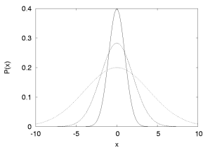
Figure 1: The Gaussian probability distribution of a free Brownian particle, located initially at $x=0$, is plotted at three later times; the width increases following the equation (1). (Copyright: Indrani Chowdhury; reproduced with permission).

Einstein’s 1905 paper on Brownian motion was not the only paper he wrote on this topic. In fact, in the opinion of leading historians of science, Einstein’s Ph.D. thesis, which was published in 1906, is perhaps more important contribution to the theory of Brownian motion than his 1905 paper. But a detailed discussion of his later papers on this subject is beyond the scope of this article.

Einstein also realized what would be the fate of kinetic theory in case experimental data disagreed with his predictions. he wrote, “…had the prediction of this movement proved to be incorrect, a weighty argument would be provided against the molecular-kinetic conception of heat”.

In 1900 Louis Bachelier’s thesis entitled “Therie de la Speculation” was examined by three of the greatest mathematician and mathematical physicists, namely, Paul Appell, Joseph Boussenesq and Henri Poincare. It was Poincare who wrote the report on that thesis which may be regarded as the pioneeing work on the application of mathematical theory of financial markets. In his thesis Bachelier postulated that stock prices execute Brownian motion and he developed a mathematical theory which was, at least in spirit, very similar to the theory Einstein developed five years later!

III.2 Smoluchowski

Unlike Einstein, Marian Smoluchowski was familiar with the literature on the experimental studies of Brownian motion. If he had not waited for testing his own theoretical predictions, the credit for developing the first theory of Brownian motion would go to him. He developed the theory much before Einstein but he decided to publish it only after he saw Einstein’s paper which contained similar ideas. In his first paper, smolu06 published in 1906, Smoluchowski also pointed out the error in the Nägeli-Ramsey objection against the original Cantoni-Delsaulx-Carbonelle argument. He clarified that each of the apparently straight segments of the Brownian trajectory is caused not by a single collision with a fluid particle, but by an enormously large number of successive kicks it receives from different fluid particles which, by rare coincidence, give rise to a net displacement in the same direction.

III.3 Perrin

Jean Perrin, togther with his students and collaborators embarked on the experimental testing of Einsteins theoretical predictions. Their first task was to prepare a colloidal suspension with dispersed particles of appropriate size. They used gamboge, a gum extract, which forms spherical particles when dissolved in water. With the samples thus prepared, Perrin not only confirmed that the root-mean-square displacement of the dispersed particles grow with time $t$ following the square-root law (1) but also made a good estimate of the Avogadro number. Einstein himself was surprised by the high level of accuracy achieved by Perrin and in a letter to Perrin he admitted “I did not believe that it was possible to study the Brownian motion with such a precision”. It is true that the critics of molecular reality were silenced not by just one set of experiments of Perrin, but by the overwhelming evidence that emerged from almost identical estimates of the Avogadro number obtained by using many different methods. For his outstanding contribution, Jean Perrin was the Nobel prize in 1926.

III.4 Langevin

In the first approximation, we can approximate the fluid by a continuum. Therefore, the classical equations of motion of the Brownian particle can be written as

$$dx/dt=v$$ (5)

$$M(dv/dt)=F_{ext}-\Gamma v$$ (6)

where, at this level of description, $\Gamma$ is treated as a phenomenological parameter. One interesting feature of this equation is that, in case of tiny particles whose inertia (i.e., mass) is negligibly small, $\Gamma v\propto F_{ext}$, a relation reminiscent of Aristotelian mechanics which was based on the assumption that it is the velocity (rather than the acceleration) which is proportional to the external force acting on it.

However, on the scale of the size of a real Brownian particle the fluid does not appear to be a continuum. In fact, a Brownian particle “sees” that the fluid is made of molecules that constantly, but discretly, strike this Brownian particle, accelerating and decelerating it perpetually. “We witness in Brownian movement the phenomenon of molecular agitation on a reduced scale by particles very large on molecular scale ” chandrasekhar . A single collision has very small effect on the Brownian particle; the Brownian motion observed under a microscope is the cumulative effect of a rapid and random sequence of large number of weak impulses. Since the number of collisions suffered by the Brownian particle is very large, we do not intend to follow its path in any detail. Instead, we would like to have a stochastic description of its movement.

Since equation (6) is a good first approximation, we assume that equation (6) correctly describes the average motion. We now incorporate the effects of the discret collisions in a stochastic manner by adding a fluctuating force (with vanishing mean) to the frictional force term:

$$M(dv/dt)=F_{ext}-\Gamma v+F_{br}(t)$$ (7)

So far as the “fluctuating force” (“noise”) $F_{br}(t)$ is concerned, we assume:
(i) $F_{br}(t)$ is independent of $v$, and
(ii) $F_{br}(t)$ varies extremely rapidly as compared to the variation of $v$. Since “average motion” is still assumed to be governed by the equation (6), we must have

$$<F_{br}(t)>=0.$$ (8)

Moreover, the assumption (ii) above implies that during small time intervals $\Delta t$, $v$ and $F_{br}$ change such that $v(t)$ and $v(t+\Delta t)$ differ infinitesimally but $F_{br}(t)$ and $F_{br}(t+\Delta t)$ have no correlation:

$$<\xi(t)\xi(t^{\prime})>=2DT\delta(t-t^{\prime})$$ (9)

where, $\xi=F_{br}/M$ and, at this level of description, $D$ is a phenomenological paranmeter. The prefactor $2$ on the right hand side of equation (9) has been chosen for later convenience. In fact, soon we shall see that, in order that the Brownian particle is in thermal equilibrium with the surrounding fluid, the constant $D$ cannot be arbitrary; only a specific choice of $D$ guarantees the approach to the appropriate equilibrium Gibbsian distribution.

Note that the spectral density

$$S(\omega)=2\int_{-\infty}^{\infty}e^{-i\omega t}<\xi(\tau)\xi(\tau+t)>dt$$ (10)

implies that, if the noise satisfies the condition (9), then $S(\omega)=4D$, independent of $\omega$. Since $S(\omega)$ is independent of the frequency $\omega$, this specific form of noise is called “white”. In more general cases, the spectral density of the noise would depend on the frequency $\omega$ and such noises are called “colored”. In the simplest formulations of the Langevin theory of Brownian motion, one assumes that $\xi(t)$ is Gaussian distributed (with vanishing mean) and with correlations of the form (9); for obvious reasons, such noises are referred to as “Gaussian white noise”. There are some advantages of the Gaussian approximation. But these are too technical to be discussed here.

What is the operational meaning of the symbol $<.>$ of averaging? The averaging is to be carried out over the distribution of the noise. This can be implemented practically in two alternative, but equivalent, ways:
either averaging over an ensemble of many systems consisting of a single Brownian particle in a surrounding fluid, or averaging over a number of Brownian particles in the same fluid, provided they are sufficiently far apart (possible at low enough density of the particles) so as not to influence each other.

What is meant by the term “solution” of a stochastic equation like the Langevin equation? Suppose, we observe a Brownian particle under a microscope over a sufficiently long time interval $0\leq t\leq T$ and obtain a record of its position $\vec{r}(t)$ as a function of time $t$. If the observations are made repeatedly, say $N$ times, we get $N$ trajectories

$$\vec{r}_{1}(t),\vec{r}_{2}(t),...\vec{r}_{N}(t).$$

In general, these trajectories are all different, i.e., for a given $t=t^{\ast}$, $\vec{r}_{1}(t^{\ast}),\vec{r}_{2}(t^{\ast}),...\vec{r}_{N}(t^{\ast})$ are all different from each other. In other words, the motion of the Brownian particle is not reproducible and, therefore, not deterministic. Then, what can physics predict about Brownian motion on the basis of the Langevin equation? Since, we are unable to make deterministic predictions we make probabilistic ones.

If we repeat the observations a large number of times,we should be able to find empirically the distribution of $\vec{r}(t)$. In other words, we can calculate the probability $P(\vec{r},t;\vec{r}_{0},\vec{v}_{0})$, which is the probability of finding the particle at position $\vec{r}$ at time $t$, given that its initial position and velocity were $\vec{r}_{0}$ and $\vec{v}_{0}$, respectively. Moreover, we can also calculate more detailed probability distributions like, for example, $P(\vec{r},\vec{v},t;\vec{r}_{0},\vec{v}_{0})$. However, we shall first look at the moments of these distributions, e.g., $<\vec{v}(t)>$, $<\vec{r}^{2}(t)>$ by using the statistical properties of noise.

Calculation of the mean-square displacement, with the given initial position $x=0$ at $t=0$, leads to the final result (I leave it as an exercise for the students to go through the steps of the calculation)

$$<x^{2}>=\biggl{(}\frac{2k_{B}T}{\Gamma}\biggr{)}\biggl{[}t-\biggl{(}\frac{1}{\gamma}\biggr{)}\biggl{(}1-e^{-\gamma t}\biggr{)}\biggr{]}.$$ (11)

Let us examine the two limiting cases. When $t\ll\gamma^{-1}$,

$$<x^{2}>\simeq(k_{B}T/M)t^{2}.$$ (12)

On the other hand, when $t\gg\gamma^{-1}$,

$$<x^{2}>\simeq(2k_{B}T/\Gamma)t.$$ (13)

Thus, the Brownian particle moves, effectively, “ballistically” for times $t\ll\gamma^{-1}$ whereas for times $t\gg\gamma^{-1}$ it moves “diffusively” with the effective diffusion coefficient $D=k_{B}T/\Gamma$. Note that the equation (13) is identical to the the equation (1) derived earlier by Einstein through his diffusion equation approach.

Thus, the Langevin equation (7) is a stochastic dynamical equation that accounts for irreversible processes. On the other hand, in principle, one can write down the equations of motion for the Brownian particle as well as that of all the other particles constituting the heat bath; each of these Hamilton’s canonical equation of motion will not only be deterministic but will also exhibit time-reversal symmetry. Note that, in the Langevin approach, one writes down only the equation (7) for the Brownian particle and does not explicitly describe the dynamics of the constituents of the heat bath. Therefore, a fundamental question is: how do the viscous damping term (responsible for irreversibility) and the random force term (which gives rise to the stochasticity) appear in the equation of motion of the Brownian particle when one “projects out” the degrees of freedom associated with the bath variables and observes the dynanics in a tiny subspace of the full phase space of the composite system consisting of the Brownian particle + Bath?

To my knowledge, the simplest derivation of the stochastic Langevin equation for a Brownian particle, starting from the mutually coupled deterministic Hamilton’s equations (which are equivalent to Newton’s equation) for the Brownian particle and the molecules of the fluid, was given by Robert Zwanzig zwanzig . For the simplicity of analytical calculations, he modelled the heat bath as a collection of harmonic oscillators each of which is coupled to the Brownian particle. The differential equations satisfied by the position $Q$ and the momentum $P$ of the Brownian particle have the general form

$$\dot{Q}={P}/{M}$$ (14)

$$dP/dt=F_{ext}+f(Q(t),\{q(t)\},\{p(t)\})$$ (15)

where $F_{ext}$ is the external force (not arising from the reservoir) while $\{q(t)\}$ and $\{p(t)\}$ denote all the positions and momenta of the harmonic oscillators constituting the reservoir. Similarly, one can also write down the equations of motion for each of the harmonic oscillators constituting the reservoir.

In principle, one can formally integrate the equations of motion for the bath variables, in terms their corresponding initial conditions, and substitute the formal solutions into the equation (15) for the Brownian particle. Even at this stage, the resulting equation is purely deterministic. But, it involves the intial positions and initial momenta of all the harmonic oscillators and, in practice, it is impossible to specify such a large number of initial conditions exactly. If we now assume that only statistical properties of these initial conditions of the bath variables are known (or, postulated) we get a differential equation for $P$ which is a slight generalization of the Langevin equation (7). This simple analytical calculation demonstrates how both the dissipative viscous drag term and the noise term appear in the equation of motion of the Brownian particle when the bath degrees of freedom are projected out.

Thus, the molecules in the fluid medium which give the random “kicks” to the Brownian particle are also responsible for its energy dissipation because of viscous drag. Therefore, it should not be surprising that these two manifestations of the fluid medium are related through the Einstein relation (2). This also answers one of puzzles faced by early investigators: in the absence of any force imposed on the Brownian particle from outside the fluid, why doesn’t it come to a complete halt in spite of the viscous drag ? The incessant random motion of the Brownian particle is maintained for ever by the delicate balance of the random kicks it gets from the fluid particles and the energy it dissipates back into the fluid via viscous drag.

III.5 Fokker-Planck versus Langevin approach

Einstein’s approach has been generalized by several of his contemporaries including Fokker, Planck, Smoluchowski and others. This general theoretical framework is now called the Fokker-Planck approach fpleqn . In this approach, one deals with a deterministic partial differential equation for a probability density. For example, suppose $P(\vec{r},\vec{v};t|\vec{r}_{0},\vec{v}_{0})$ be the conditional probability that, at time $t$, the Brownian particle is located at $\vec{r}$ and has velocity $\vec{v}$, given that its initial (i.e., at time $t=0$) position and velocity were $\vec{r}_{0},\vec{v}_{0}$. Since the total probability integrated over all space and all velocities is conserved (i.e,, does not change with time), the probability density $P$ satisfies an equation of continuity

$$\frac{\partial P}{\partial t}+\frac{\partial J_{p}}{\partial x}=0$$ (16)

where $J_{p}$ is the corresponding probability current. Note that the probability density and the probability current density are analogs of the electrical charge density and electrical current density in electrodynamics where it follows from the conservation of electrical charge in the system.

The probability current density $J_{p}$ gets contributions from two sources: the diffusion current, given by Fick’s law, is caused by the concentration gradient, while the drift current is imposed by the externally applied force $F$. Thus,

$$J_{p}(x,t)=-D\biggl{(}\frac{\partial P}{\partial x}\biggr{)}+\biggl{(}\frac{F}{\Gamma}\biggr{)}P$$ (17)

where the first and the second terms on the right hand side arise from diffusion and drift, respectively. The expression (17) can be recast in several alternative, but equivalent, forms using the relation between the force $F$ and the corresponding potential $U$, namely, $F=-dU/dx$ and the Einstein relation $\Gamma D=k_{B}T$.

In contrast, the Langevin approach langevin is based on a stochastic differential equation for the individual Brownian particle and is, in spirit, closer to Newton’s equation. Because of the stochasticity, unique initial condition does not lead to a unique trajectory of the particle.

Stochasticity can enter into a differential equation either as an additive term or as a multiplicative factor. For example, the Langevin equation for a Brownian Harmonic oscillator in one-dimension is given by

$$M\frac{d^{2}X}{dX^{2}}=-M\omega^{2}X-\Gamma\frac{dX}{dt}+F_{B}(t)$$ (18)

where the random Brownian force $F_{B}(t)$ introduces stochasticity that appears as an additive term in the dynamical equation. In contrast, the Langevin equation for the so-called Kubo oscillator is given by

$$M\frac{d^{2}X}{dX^{2}}=-M\omega_{B}^{2}(t)X-\Gamma\frac{dX}{dt}$$ (19)

where frequency $\omega_{B}(t)$ is random and, thus, stochasticity enters into the dynamical equation as a multiplicative factor.

IV Beyond translation- rotation and shape fluctuations

In undergraduate mechanics courses in colleges (or universities), normally, a student first learns Newtonian mechanics of point particles which also describes the motion of the center of mass of extended objects. Then, one learns the deal with the rotational motion of rigid bodies. Finally, a student is exposed to the mechanics of deformable bodies, i.e., elastic solids and fluids. So far in this article we have considered only the translational motion of the center of mass of the Brownian particles. In this section we shall consider rotational Brownian motion of rigid particles and the shape fluctuations of soft materials caused by the Brownian motion of these deformable bodies.

IV.1 Rotational Brownian motion of rigid bodies

To my knowledge, one of the earliest direct experimental observations of the rotational Brownian motion was made by Gerlach gerlach using a tiny mirror fixed on a very fine wire; some of the fundamental questions on this problem were addressed theoretically soon thereafter by Uhlenbeck and Goudsmit uhlenrot . This is a relatively simple problem because the rotation involves only a single angle $\theta$ which measures the angular deflection. The corresponding Langevin equation has the form

$$I\biggl{(}\frac{d^{2}\theta}{dt^{2}}\biggr{)}={\cal T}_{ext}-G\theta-\alpha\biggl{(}\frac{d\theta}{dt}\biggr{)}+{\cal T}_{br}$$ (20)

where $I$ is the moment of inertia of the oscillator, $\alpha$ is the friction coefficient, $G$ is the torsional elastic constant of the fiber, ${\cal T}_{ext}$ is the external torque and ${\cal T}_{br}$ is the Brownian (i.e., random) torque. Each term of this Langevin equation is the rotational counterpart of the corresponding term in the Langevin equation (7) for translational Brownian motion.

Interestingly, three quarters of a century later the problem of rotational Brownian motion of a mirror was reinvestigated by replacing air by a fluidized granular medium. In this novel experiment granular the torsion oscillator was immersed in a container filled with glass beads and the noisy vertical vibration of the container took place at frequencies much higher than the natural frequency of the torsion oscillator.

The Langevin equation for the more general cases of rotation of a rigid body in three dimensions has more complex form. Recall that the rotational motion of a macroscopic asymmetrical object is given by the Euler equation. The corresponding Euler-Langevin equation for rotational Brownian motion has the general form

$$\frac{d\vec{L}}{dt}+\vec{\omega}\times\vec{L}={\cal T}_{ext}-\Gamma\omega+{\cal T}_{br}(t)$$ (21)

with $\vec{L}=I\omega$, where $I$ is the moment of inertia of the body and $\omega$ is its angular velocity; ${\cal T}_{ext}$ is the externally imposed torque while ${\cal T}_{br}(t)$ is the random noise torque. For the sake of simplicity one often assumes a Gaussian white noise torque ${\cal T}_{br}(t)$.

How should we write down the Fokker-Planck equation corresponding to the Euler-Langevin equation (21)? Let us denote by the symbol $S^{\prime}$ a principal coordinate system fixed in the rigid body. The orientation of the body can be specified by the Euler angles $\Omega_{1},\Omega_{2},\Omega_{3}$ of $S^{\prime}$ with respect to the laboratory coordinate system $S$. We can now define the probability density $P(\Omega_{1}(t),\Omega_{2}(t),\Omega_{3}(t);\omega_{1}(t),\omega_{2}(t),\omega_{3}(t)|\Omega_{1}(0),\Omega_{2}(0),\Omega_{3}(0);\omega_{1}(0),\omega_{2}(0),\omega_{3}(0))$ which represents the conditional probability that, at time $t$, the Euler angles are $\Omega_{1}(t),\Omega_{2}(t),\Omega_{3}(t)$ and the angular velocities $\omega_{1}(t),\omega_{2}(t),\omega_{3}(t)$, given that the corresponding initial values were $\Omega_{1}(0),\Omega_{2}(0),\Omega_{3}(0)$ and $\omega_{1}(0),\omega_{2}(0),\omega_{3}(0)$, respectively.

The problem of rotational Brownian motion of a sphere was briefly mentioned in a paper published by Einstein in 1906 einstein06 . Investigaton of the rotational Brownian motion in the context of dielectric relaxation was initiated by Peter Debye and extended by many authors in the second half of the twentieth century conel .

Another related problem is the relaxational dynamics of large single-domain particles in rocks rock . Each of these particles consists of a large number of individual moments all aligned parallel to each other such that the particle posseses a giant magnetic moment. Since the particle is embedded in a solid matrix, it cannot rotate physically but the direction of the magmetic moment can undergo Brownian rotation. A collection of such single-domain particles will be aligned parrel to the externally applied magnetic field. Then, after the field is switched off, the remanent magnetization $M_{r}$ will vanish as

$$M_{r}=M_{s}e^{-t/\tau},$$ (22)

where $M_{s}$ is the magnetization of a non-relaxing particle, $t$ is the time elapsed after the field is switched off and

$$\tau=\tau_{0}e^{AV/k_{B}T}$$ (23)

is the relaxation time where $V$ is the volume of the particle and $\tau_{0}\sim 10^{-9}$ sec. Therefore, varying $V$ and/or $T$, the relaxation time $\tau$ can be made to vary from $10^{-9}$ sec. to millions of years.

It was pointed out by Louis Neel that, at a given temperature $T$, the particle magnetization will appear “blocked” (i.e., frozen in time) in any dynamic experiment where the frequency of the measurement $\omega_{m}$ is such that $\tau\gg\omega_{m}^{-1}$.

Blocking of the magnteization of the super-paramagnetic particles finds important applications in paleomagnetism (geomagnetism), as the history of the earth’s magnetic field remains frozen in the rocks. During the early stage of the formation of the rock at a relatively higher temperature, the magnetic particles exist in thermal equilibrium with the Earth’s magnetic field, but later, as the rock cools, the magnetization of these particles get “blocked” and they retain the memory the direction of the Earth’s magnetic field.

IV.2 Brownian motion of deformable bodies: shape fluctuations

A linear polymer is a simple example of a deformable body which is, effectively, one dimensional. The Brownian forces acting on such an object in aqueous medium can give rise to random wiggling, i.e., random fluctuations in its shape. The random Brownian forces tend to induce wiggles in the polymer chain while the bending stiffness tends to restore its linear shape. These two competing effects determines overall conformation of the polymer chain. One of the most important effects of its Brownian wiggling is that, even in the absence of any energy cost for creating such wiggles, the polymer behaves, effectively, as a spring where its spring constant is temperature-dependent and the corresponding restoring force it exerts is of purely entropic origin.

Suppose $\hat{n}(0)$ and $\hat{n}(s)$ are the unit normals to the polymer at two points on the polymer separated by a distance $s$ measured along the contour of the chain. Then, the correlation between the orientations of these two unit normals decreases exponentially with increasing $s$, i.e., proportional to $exp(-s/\xi_{p})$ where $\xi_{p}$, the persistence length, is determined by the ratio of the bending stiffness energy and the thermal energy $k_{B}T$. If the total length of the polymer is $L$, it appears stiff when $L<<\xi_{p}$ whereas it appears floppy when $L>>\xi_{p}$. Microtubules have very long persistence length.

Similarly, Brownian motion of a soft membrane, e.g., the plasma membrane of a red-blood cell, manifests as “flickering” of the, effectively, two-dimensional elastic sheet. The Brownian shape fluctuations of soft membranes have many important consequences. For example, consider a stack of such membranes which have a tendency to stick to each other because of the ubiquitous Van der Waals attractions. However, at all non-zero temperatures the Brownian shape fluctuations cause the membranes to bump against each other; the higher is the temperature the stronger is the, effectively, repulsive entropic force. As a consequence of this competition between the two forces, an unbinding phase transition takes place in the system at a characteristic temperature as the temperature is raised from below.

V Brownian motion in external static potential

Translational Brownian motion of a particle under the influence of an external linear potential of the form $U(x)=ax$ is relevant, for example, in the context of sedimentation of colloidal particles under gravity chandrasekhar . Brownian motion of a harmonically bound particle uhlenorn , i.e., a particle subjected to a quadratic potential of the form $U(x)=ax^{2}$, is a reasonably good model for the dynamics of tiny spherical dielectric particle trapped by an optical tweezer. In order to satisfy the law of equipartition of energy in thermodynamic equilibrium, $<x^{2}>$ approaches the value $k_{B}T/(m\omega^{2})$ in the limit of extremely long time limit; Uhlenbeck and Ornstein uhlenorn derived the exact expression valid for all times and, hence, showed how $<x^{2}>$ approaches the asymptotic value with the passage of time.

The potential $U(x)=-ax^{2}+bx^{4}$ has two equally deep minima which are separated from each other by an energy barrier; Brownian motion of a particle subjected to such a potential leads to noise assisted transitions, back and forth, from one well to the other. The average waiting time $T_{K}$ between two successive noise-induced transitions increases exponentially with the increase of the barrier height. Noise-induced transitions in bistable systems have found applications in a wide variety of systems; we shall call $T_{K}$ as the Kramers time in honor of Hendrik Kramers who considered such problems first in the context of chemical reaction rate theory in his classic paper entitled “Brownian motion in a field of force and the diffusion model of chemical reactions” hanggi ; melnikov .

Kramers was not the first to consider noise-induced transitions from a potential well. In fact, in 1935, Becker and Döring studied the problem noise-assisted hopping of a barrier to escape from a metastable state. The problem of noise-induced transitions in systems with metastable, bistable or multistable systems has a long history with abundant examples of unintentional rediscoveries and rederivation of results by experts from different disciplines, often using different terminologies landauer . Nevertheless, this shows the breadth of coverage of this multidisciplinary umbrella and the wide range of applicability of the concepts and techniques.

VI Brownian motion in time-dependent potential

In the preceeding section we have considered Brownian motion in static (time-independent) external potential. However, two of the hottest topics in the area of Brownian motion which have kept many physicists busy for the last quarter of a century, are related to Brownian motion in time-dependent potentials. In the following two subsections we briefly discuss these two phenomena, namely, stochastic resonance and Brownian ratchet.

VI.1 Stochastic resonance and applications

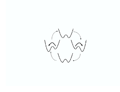
Figure 2: The back and forth tilting of the bistable potential in one cycle of the periodic focing. (Copyright: Indrani Chowdhury; reproduced with permission).

Let us begin with a Brownian particle subjected to a bistable potential. Suppose a small amplitude periodic forcing is added so that the left and the right wells periodically exchange their relative stability as shown in fig.2. Let $T_{p}=2\pi/\Omega_{p}$ be the time period of the periodic forcing. Then, the potential $U(x)$ is given by

$$U(x,t)=\frac{a}{2}x^{2}-\frac{b}{4}x^{4}-A_{0}x~{}cos(\Omega_{p}t)$$ (24)

and the corresponding Langevin equation for the Brownian particle is

$$m\frac{d^{2}x}{dt^{2}}=-ax+bx^{3}+A_{0}~{}cos(\Omega_{p}t)+F_{br}$$ (25)

Note that the periodic forcing is too weak to induce transition in the position of the particle from one well to the other without assistance from noise. However, in the presence of noise, even in the absence of forcing, noise-induced transition from one well to the other goes on. Now, extending the concept of resonance, we introduce the concept of stochastic resonence by the condition

$$2T_{K}(D)=T_{p}$$ (26)

where $T_{K}$ is the Kramers time and it depends on the strength $D$ of the noise gammaitoni ; moss .

The phenomenon of stochastic resonance has been demonstrated directly in laboratory experiments libchab . A micron-size dielectric bead is used as the Brownian particle and a bistable potential is created using two optical (laser) traps. The most important quantity characterizing a stochastic resonance is the signal-to-noise (SNR) ratio. The signature of a stochastic resonance is that the SNR, which vanishes in the absence of noise, rises with the increase of noise intensity and exhibits a maximum at an optimum level of noise intensity; on further increase of noise intensity SNR decreases because of the randomization caused by the noise. In other words, contrasy to naive expectations, noise can have a constructive effect in enhancing the signal over an appropriately chosen window of noise intensity. Not surprisingly, it finds applications in electrical engineering. Moreover, many organisms seem to use stochatic resonance for sensory perception; these include, for example, electro-receptors of paddlefish mechano-receptors of crayfish, etc.

Stochastic resosnance has been evoked to explain the periodic occurrence of Ice age on earth; the period is estimated to be approximately $100,000$ years. Suppose the ice-covered and water-covered earth correspond to the two local minima. Eccentricity of the earth’s orbit (and, therefore, incoming solar radiation) varies periodically with a period of about $T_{p}\simeq 100,000$ years. But, this variation is too weak to cause the transition from ice-covered to water-covered earth and vice versa. It has been suggested that random noise in the climatic conditions can give rise to a stochastic resonance causing a transition between the two local minima with a period of about 100,000 years.

VI.2 Brownian ratchet and applications

Let us now consider a Brownian particle subjected to a time-dependent potential, in addition to the viscous drag (or, frictional force). The potential switches between the two forms (i) and (ii) shown in fig.3. The sawtooth form (i) is spatially periodic where each period has an asymmetric shape. In contrast, the form (ii) is flat so that the particle does not experience any external force imposed on it when the potential has the form (ii). Note that, in the left part of each well in (i) the particle experiences a rightward force whereas in the right part of the same well it is subjected to a leftward force. Moreover, the spatially averaged force experienced by the particle in each well of length $\ell$ is

$$<F>=-\frac{1}{\ell}\int_{0}^{\ell}\biggl{(}\frac{\partial U}{\partial x}\biggr{)}dx$$

$$=U(0)-U(\ell)=0$$ (27)

because of the spatially periodic form of the potential (i). What makes this problem so interesting is that, in spite of vanishing average force acting on it, the particle can still exhibit directed, albeit noisy, rightward motion.

In order to understand the underlying physical principles, let us assume that initially the potential has the shape (i) and the particle is located at a point on the line that corresponds to the bottom of a well. Now the potential is switched off so that it makes a transition to the form (ii). Immediately, the free particle begins to execute a Brownian motion and the corresponding Gaussian profile of the probability distribution begins to spread with the passage of time. If the potential is again switched on before the Gaussian profile gets enough time for spreading beyond the original well, the particle will return to its original initial position. But, if the period during which the potential remains off is sufficiently long, so that the Gaussian probability distribution has a non-vanishing tail overlapping with the neighbouring well on the right side of the original well, then there is a small non-vanishing probability that the particle will move forward towards right by one period when the potential is switched on.

In this mechanism, the particle moves forward not because of any force imposed on it but because of its Brownian motion. The system is, however, not in equilibrium because energy is pumped into it during every period in switching the potential between the two forms. In other words, the system works as a rectifier where the Brownian motion, in principle, could have given rise to both forward and backward movements of the particle in the multiples of $\ell$, but the backward motion of the particle is suppressed by a combination of (a) the time dependence and (b) spatial asymmetry (in form (i)) of the potential. In fact, the direction of motion of the particle can be revsered by replacing the potential (i) by the potential (iii) shown in fig.4.

The mechanism of directional movement discussed above is called a Brownian ratchet reiman for reasons which we shall now clarify. The concept of Brownian ratchet was popularized by Feynman through his lectures feynman although, historically, it was introduced by Smoluchowski smolurat . Consider the ratchet and pawl arrangement shown in fig.5. The random bombardment of the vanes by the air molecules gives rise to torques which fluctuates randomly both in magnitude and direction. Because of the asymmetric shape of each of the teeth, it may appear, the ratchet would move countercloclowise more easily than clockwise (when viewed from the left side) leading to its directed counterclockwise, albeit noisy, rotation. In principle, it should then be possible to exploit such directed rotation to perform mechanical work. However, any such device, if it really existed, would violate the second law of thermodynamics because it would extract thermal energy from its environment, by cooling the environment spontaneously, and convert that energy into mechanical work. Feynman resolved the apparent paradox by pointing out that both the clockwise and counterclockwise rotations are actually equally likely because the pawl also executes random Brownian motion because of the random extension and compression of the spring that keeps it pressed against the wheel of the ratchet. A linear design of the Brownian ratchet is shown in fig.6

Figure 3: The two forms of the time-dependent potential used for implementing the Brownian ratchet mechanism. (Copyright: Indrani Chowdhury; reproduced with permission).

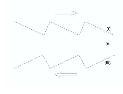
Figure 4: The direction of the motion of the particle in a Brownian ratchet is determined by the form of the asymmetry of the potential in each period. (Copyright: Indrani Chowdhury; reproduced with permission).

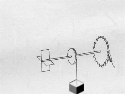
Figure 5: Feynman’s ratchet and pawl arrangement. (Copyright: Indrani Chowdhury; reproduced with permission).

Brownian ratchet has its counterpart in the abstract theory of games. In particular, Juan Parrondo parrondo proposed a game with two separate rules, say $A$ and $B$, of the game. Even in situations where both the rules will ruin the gambler, Parrondo showed that the gambler can win by using the rules $A$ and $B$ alternately. It is not difficult to map this problem onto the Brownian ratchet mechanism depicted in fig. (3) and the winning of the gambler corresponds to the directed movement of the Brownian particle in fig.(3).

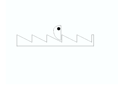
Figure 6: A linear ratchet and pawl arrangement. (Copyright: Indrani Chowdhury; reproduced with permission).

The ratcheting via time-dependent potential discussed above it not merely a theoretical possibility but nature exploits this for driving a class of molecular motors inside cells of living organisms; this includes KIF1A, a family of kinesin motor proteins chowreso . Such molecular motors move along microtubule filaments just as trains move along their tracks.

A Brownian-ratchet based mechanism has been proposed simon for translocation of proteins across membranes. This is easy to understand using a picture similar to the ratchet shown in the fig.6. Proteins, are known to unfold before translocation through a narrow pore in the membrane. Once the tip of the protein successfully penetrates the membrane, it can translocate through Brownian motion provided there exist some mechanism to rectify its backward movements. Several possible mechanisms for such rectification have been proposed including binding of chaperonins at designated binding sites along the translocated part of the macromolecule chowreso .

ATP is the energy currency of almost all eukaryotic cells and the cell synthesizes ATP from the raw materials using a machine, called ATP synthase, which is bound to the mitochondrial (chloroplast) membrane of animal (plant) cells. To my knowledge, this is smallest among all the natural and man made rotary motors. This complex motor actually consists of two reversible parts, namely $F_{0}$ and $F_{1}$, which are coupled to each other. A Brownian-ratchet mechanism has been suggested oster for the rotary motor $F_{0}$. Detailed structure and function of this natural nano-motor will be considered in a separate article chowreso .

VII Summary and conclusion

What started as a curiosity of microscopists, who were baffled by the random movements of the pollen grains in water, turned out to be one of the most challenging scientific problems that could not be solved by anybody till the beginning of the twentieth century. It was Albert Einstein who, in one of his three revolutionary papers of 1905, published the correct theory of Brownian motion. His theoretical predictions were confirmed by a series of experiments on colloidal dispersions by Jean Perrin and his collaborators. These investigation of Brownian motion in collidal dispersions not only helped in silencing the critics of the molecular kinetic theory of matter but also laid down the foundation of statistical mechanics.

By the end of the first quarter of the twentieth century quantum theory became the darling of the majority of the physicists and the colloidal suspensions lost its appeal. Over the next quarter of a century progress was rather slow but steady. However, in the second half of the twentieth century, motivated partly by the industrial demand for novel materials, physicists and engineers discovered great potential of the soft materials frey , including colloids which gradually regained its past glory haw . Moreover, revolution in optical microscopy in the last ten years has provided a glimpse of the cellular interior, a wonderland dominated by Brownian motion. Preliminary explorations in this new frontier of research indicate that, instead of being a nuisance, the Brownian motion is, perhaps, fully exploited by Nature to its advantage not merely to survive but to thrive. Brownian motion of pollen grains does not arise from any process of life but some of the least understood processes of life, including the train-like motion of the biomolecular motors on the filamentary tracks, may not be possible without Brownian motion!

Acknowledgements: I thank Manoj Harbola and Ambarish Kunwar for a critical reading of the manuscript.

References

- (1) J. Stachel, Einstein’s miraculous year: Five Papers that changed the face of physics (Princeton University Press, 1998).
- (2) A. Einstein, Annalen der Phys. 17, 549 (1905).
- (3) J. Bronowski, The ascent of man (Little Brown and Co., 1976).
- (4) C. A. Gearhart, Am. J. Phys. 58, 468 (1990).
- (5) M. Smoluchowski, Ann. Phys. paris, 21, 772 (1906).
- (6) S. Chandrasekhar, Rev. Mod. Phys. 15, 1 (1943).
- (7) R. Zwanzig, J.Stat. Phys. 9, 215 (1973).
- (8) H. Risken, The Fokker-Planck Equation, (Springer, 2004).
- (9) W.T. Coffey, Yu. P. Kalmykov and J.T. Waldron, The Langevin Equation, Second edition, (World Scientific, 2004).
- (10) W. Gerlach, Naturwiss., 15, 15 (1927).
- (11) G.E. Uhlenbeck and S. Goudsmit, Phys. Rev. 34, 145 (1929).
- (12) G. D’Anna, P. mayor, A. Barrat, V. Loreto and F. Nori, Nature, 424, 909 (2003).
- (13) A. Einstein, Ann. der Phys. 19, 371-381 (1906).
- (14) J. McConnell, Rotational Brownian motion and dielectric theory, (Academic Press, 1980).
- (15) D.J. Dunlop and O. Ozdemir, Rock magnetism (Cambridge University Press, 2001).
- (16) G.E. Uhlenbeck and L.S. Ornstein, Phys. Rev. 36, 823 (1930).
- (17) P. Hänggi and P. Talkner, Rev. Mod. Phys. 62, 251 (1990).
- (18) V.I. Melnikov, Phys. Rep. 209, 1 (1991).
- (19) R. Landauer, in: Noise in nonlinear dynamical systems, vol.1, eds. F. Moss and P.V.E. McClintock (Cambridge university press, 1989).
- (20) L. Gammaitoni, P. Hänggi, P. Jung, Rev. Mod. Phys. 70, 223 (1998).
- (21) V.S. Anishchenko, A.B. Neiman, F. Moss and L. Schimansky-Geier, Phys. Uspekhi, 42, 7 (1999).
- (22) A. Simon and A, Linchaber, Phys. Rev. lett. 68, 3375 (1992).
- (23) P. Reimann, Phys. Rep. 361, 57 (2002).
- (24) R.P. Feynman, The Feynman Lectures on Physics, vol.1 (Addison-Wesley, 1963).
- (25) M. Smoluchowski, Physik. Z. 13, 1069 (1912).
- (26) J. M. R. Parrondo and L. Dinis, Contemp. Phys. 45, 147 (2004).
- (27) Please see the elementary review article by D. Chowdhury, (to be be published).
- (28) S.M. Simon, C. S. Peskin and G.F. Oster, Proc. Natl. Acad. Sci.USA, 89, 3770 (1992).
- (29) G. Oster and H. Wang, in:Molecular Motors, ed. M. Schliwa (Wiley-VCH, 2003).
- (30) E. Frey and K. Kroy, Ann. Phys. (Leipzig) 14, 20 (2005).
- (31) M.D. Haw, J. Phys. Condens. matter, 14, 7769 (2002).