Pairing between Atoms and Molecules in Boson-Fermion Resonant Mixture

Abstract

We consider a mixture of fermionic and bosonic atoms nearby interspecies Feshbach resonances, which have been observed recently in ⁶Li-²³Na mixture by MIT group, and in ⁴⁰K-⁸⁷Rb mixture by JILA group. We point out that the fermion-boson bound state, namely the heteronuclear molecules, will coexist with the fermionic atoms in a wide parameter region, and the attraction between fermionic atoms and molecules will lead to the formation of atom-molecule pairs. The pairing structure is studied in detail, and, in particular, we highlight the possible realization of the Fulde-Ferrel-Larkin-Ovchinnikov state in this system.

Introduction. In the latest few years ultracold atomic gases nearby Feshbach resonance have attracted considerable attention, since Feshbach resonance can be utilized to achieve strongly interacting quantum gases exhibiting universal properties, to produce Bose-Einstein condensation of molecules from atomic gasesBEC , and to study the physics of BEC-BCS crossoverBCS ; BEC-BCS . While most present experimental and theoretical works focus on the resonance between atoms of the same species, interspecies Feshbach resonances were also observed recently in collisions between fermionic ⁶Li and bosonic ²³Na by MIT groupketterle , and in collisions between fermionic ⁴⁰K and bosonic ⁸⁷Rb by JILA groupJin . These interspecies Feshbach resonances arise from the fermion-boson bound states, which are called heteronuclear molecules. In this Rapid Communication, we will show that the fermionic atoms and molecules will coexist in a wide parameter region, and they will form atom-molecule pairs and exhibit superfluidity, provided that the life-time of molecules can be long enough to reach equilibrium. Particularly, the system is a good candidate for realization of the Fulde-Ferrell-Larkin-Ovichinnikov (FFLO) state, owing to the mass difference between atom and molecule, as well as the tunable molecular binding energy.

In the study of superconductor with mismatched Fermi surfaces of different spins, FFLO state was proposed by Fulde and FerrellFF , and by Larkin and OvchinnikovLO independently. The distinct features of this state include (i) the center-of-mass momentum of each pair is nonzero, and thus the order parameter has a periodic space modulation; (ii) there are unpaired normal fermions coexisting with paired superfluid fermions. Stimulated by these exotic features, experimental condensed matter physicists have paid a lot of efforts on searching this state in various materials in the past decades, and until recently some evidences of discovering this state in $\text{CeCoIn}_{5}$ have been reportedCeCoIn . This state has also been studied in the discussion of color superconductivity and pulsars. These progresses have been systematically summarized in a latest review article Ref.RMP . Recently, the realization of the FFLO state in the mixture of two-component fermions has been suggested Combescot ; Mizushima , where the Fermi surface mismatch is controlled by unequal population of different components, and the experimental signatures of the FFLO state in cold atoms experiments have also been discussedMizushima . Besides, there are also some other proposes for the pairing problem with mismatched Fermi surfaces, such as the breached-pair stateBP and pairing with deformed Fermi surfacedefomation . Particularlly the energetic and dynamic stability of the breached-pair state have been discussed a lot in some recent literaturesBP .

Setting up the model. We consider a uniform mixture of bosonic atoms (b.a.) and fermionic atoms (f.a.). Away from the resonance, the properties of such a mixture has been extensively discussed beforeBFmixture . By introducing the operator $\hat{\Phi}$ for the b.a., and the operator $\hat{\Psi}_{a}$ for the f.a., this mixture can be described by

$$\hat{H}_{\text{A}}=\int d^{3}{\bf r}\left[\frac{\hbar^{2}}{2m_{1}}|\nabla\hat{\Psi}_{a}|^{2}+\frac{\hbar^{2}}{2m_{2}}|\nabla\hat{\Phi}|^{2}\right.$$

$$\left.+g_{0}\hat{\Phi}^{\dagger}\hat{\Phi}^{\dagger}\hat{\Phi}\hat{\Phi}+g_{1}\hat{\Psi}^{\dagger}_{a}\hat{\Psi}_{a}\hat{\Phi}^{\dagger}\hat{\Phi}\right],$$ (1)

where $g_{0}$ is the strength of the self-interaction between b.a, $g_{1}$ is the strength of interaction between b.a. and f.a., and $m_{1}$ and $m_{2}$ are the masses of f.a. and b.a. respectively. Nearby the resonance, the process that converts two atoms into a heteronuclear molecule (h.m.) should be incorporated. In the spirit of the two-channel modelHolland , we introduce an independent fermionic operator $\hat{\Psi}_{m}$ for this molecule, and describe the resonance process as

$$\hat{H}_{\text{AM}}=\alpha\int d^{3}{\bf r}\left(\hat{\Psi}^{\dagger}_{m}\hat{\Phi}\hat{\Psi}_{a}+\hat{\Psi}^{\dagger}_{a}\hat{\Phi}^{\dagger}\hat{\Psi}_{m}\right).$$ (2)

And finally the molecules are described by

$$\hat{H}_{\text{M}}=\int d^{3}{\bf r}\left[\frac{\hbar^{2}}{2m_{m}}|\nabla\hat{\Psi}_{m}|^{2}+\mu_{0}\hat{\Psi}^{\dagger}_{m}\hat{\Psi}_{m}+g_{2}\hat{\Psi}^{\dagger}_{m}\hat{\Psi}_{m}\hat{\Phi}^{\dagger}\hat{\Phi}\right].$$ (3)

Here the mass $m_{m}$ of h.m., which equals $m_{1}+m_{2}$, will be much larger than $m_{1}$ provided that $m_{2}$ is times larger than $m_{1}$. $g_{2}$ is the interaction strength between h.m. and b.a., and the molecular binding energy $\mu_{0}$ can be tuned by an external magnetic field. Therefore the total Hamiltonian is given by $\hat{H}=\hat{H}_{\text{A}}+\hat{H}_{\text{M}}+\hat{H}_{\text{AM}}$. Since we are mostly interested in the behavior of the fermions in a bosonic background, we consider the situation that the density of bosons $n_{0}$ is much larger than the density of fermions $n$, and therefore we can neglect the feedback on bosons safely. The opposite situation where $n$ is comparable to $n_{0}$ has been considered recentlyPowell , and the mean-field solution of the equal mixing case has also been providedStoof .

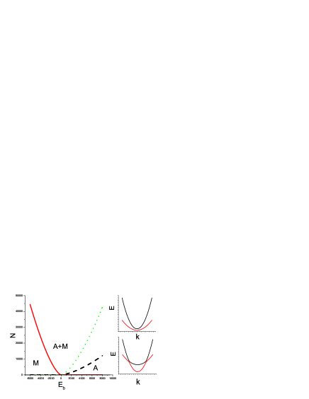
Figure 1: (color online) The mean-field $N-E_{\text{b}}$ phase diagram. Below the red solid line is the pure fermionic molecules phase; below the black dash line is the pure fermionic atoms phase, and in the region between the solid line and dash line atoms and molecules coexist. In the left-hand side of the dotted line, the Fermi momentum of atoms $k_{\text{Fa}}$ is smaller than the Fermi momentum of molecules $k_{\text{Fm}}$. The two insets schematically show the dispersion relations $\epsilon_{\pm}({\bf k})$, with $E_{\text{b}}<0$ for the upper one and $E_{\text{b}}>0$ for the lower one. The momentum $k$ is in the unit of $k_{0}=L/(2\pi)$, where $L$ is the length of the system, and the energy is in the unit of $\hbar^{2}k_{0}^{2}/(2m_{1})$. All the figures in this paper are plotted for ⁴⁰K-⁸⁷Rb mixture.

The mean-filed solution. At nearly zero temperature, the bosonic atoms are condensed. Adopting the standard Bogoliubov approximation, we expand the operator $\hat{\Phi}$ as $\sqrt{n_{0}}+\sum_{{\bf k}}e^{i{\bf k}{\bf r}}\hat{\Phi}_{{\bf k}}$. Neglecting some constants, the Hamiltonian at the mean-field level turns out to be $\hat{H}_{0}=\sum_{{\bf k}}\epsilon_{a}({\bf k})\hat{\Psi}^{\dagger}_{a{\bf k}}\hat{\Psi}_{a{\bf k}}+\epsilon_{m}({\bf k})\hat{\Psi}^{\dagger}_{m{\bf k}}\hat{\Psi}_{m{\bf k}}+\alpha\sqrt{n_{0}}(\hat{\Psi}^{\dagger}_{a{\bf k}}\hat{\Psi}_{m{\bf k}}+\hat{\Psi}^{\dagger}_{m{\bf k}}\hat{\Psi}_{a{\bf k}}),$ where $\epsilon_{a}({\bf k})$ denotes $\hbar^{2}{{\bf k}}^{2}/(2m_{1})$, and $\epsilon_{m}({\bf k})$ denotes $\hbar^{2}{{\bf k}}^{2}/(2m_{m})+E_{b}$. Here the binding energy $\mu_{0}$ is normalized to $E_{\text{b}}$ by the mean-field interactions, i.e. $E_{{\text{b}}}=\mu_{0}-g_{1}n_{0}+g_{2}n_{0}$. This quadratic Hamiltonian can be easily solved, which yields

$$\epsilon_{\pm}=\frac{1}{2}\left[\epsilon_{a}({\bf k})+\epsilon_{m}({\bf k})\pm\sqrt{(\epsilon_{a}({\bf k})-\epsilon_{m}({\bf k}))^{2}+4\alpha^{2}n_{0}}\right],$$ (4)

and they are shown in the insets of Fig. 1. Owing to the large mass difference, $|\epsilon_{a}({\bf k})-\epsilon_{m}({\bf k})|$ is usually very large unless ${\bf k}$ is very close to ${\bf k}_{\text{c}}$ where $\epsilon_{a}({\bf k})$ crosses $\epsilon_{m}({\bf k})$, the dispersion relations $\epsilon_{\pm}({\bf k})$ thus can be well approximated by $\epsilon_{a(m)}({\bf k})$ when $|k-k_{\text{c}}|\gg 2\alpha\sqrt{n_{0}}m_{1}m_{m}/(m_{2}\hbar^{2}k_{\text{c}})$, as can be seen from the Fig. 1. For a narrow resonance, this approximation is valid in the momentum region where the atom-molecule pairs are formed.

It is noticed that the total number of fermionic atoms, including those in the scattering states and in the bound state, is conserved during the resonance process, i.e. $\hat{\Psi}^{\dagger}_{a}\hat{\Psi}_{a}+\hat{\Psi}^{\dagger}_{m}\hat{\Psi}_{m}=N$, and these fermions fill the Fermi sphere with respect to $\epsilon_{\pm}({\bf k})$ at zero temperature. Thus we obtain the mean-field phase diagram for different $N$ and $E_{\text{b}}$ shown in Fig. 1, from which one can see that in a wide range the atoms and molecules coexist in the system. This feature, contrasting with the Feshbach resonance between the atoms of the same species, arises from the fact that both atoms and molecules in this system should obey the Pauli exclusive principle. Moreover, the Fermi surfaces difference $\Delta k_{F}$, which is defined as $k_{\text{Fm}}-k_{\text{Fa}}$, is given by $(\sqrt{2m_{\text{m}}(\mu-E_{\text{b}})}-\sqrt{2m_{1}\mu})/\hbar$ for fixed chemical potential $\mu$, and increases as the decrease of $E_{\text{b}}$. This is of crucial importance for the discussion of atom-molecule pairng below.

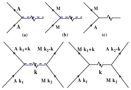
Figure 2: Upper: A diagrammatical illustration of the conventional scattering processes (a-b) and the Feshbach resonance process(c). Lower: The effective interaction between fermions owing to exchange of density fluctuations. The straight solid lines denote the propagate of Fermions, the twist solid lines denote the propagate of uncondensed Bosons, while the dotted lines denote the condensed Bosons.

Condensate fluctuation and the attractive interactions. We now incorporate the coupling between fermions and the condensate fluctuations illustrated in Fig. 2, which includes (a) density-density interaction between f.a. and b.a., $g_{1}\sqrt{n_{0}}\hat{\Psi}^{\dagger}_{a,{\bf k}_{2}}\hat{\Psi}_{a,{\bf k}_{1}}(\hat{\Phi}^{\dagger}_{{\bf k}_{1}-{\bf k}_{2}}+\hat{\Phi}_{{\bf k}_{2}-{\bf k}_{1}})$; (b) density-density interaction between h.m. and b.a., $g_{2}\sqrt{n_{0}}\hat{\Psi}^{\dagger}_{m,{\bf k}_{2}}\hat{\Psi}_{m,{\bf k}_{1}}(\hat{\Phi}^{\dagger}_{{\bf k}_{1}-{\bf k}_{2}}+\hat{\Phi}_{{\bf k}_{2}-{\bf k}_{1}})$, and (c) the Feshbach resonance, $\alpha(\hat{\Psi}^{\dagger}_{m,{\bf k}_{2}}\hat{\Phi}_{{\bf k}_{2}-{\bf k}_{1}}\hat{\Psi}_{a,{\bf k}_{1}}+\text{h.c.})$. Considering the second order processes that exchange bosonic fluctuations between fermions, an effective interaction between f.a. and h.m. will be inducedFeynman , which can be described by following effective Hamiltonian

$$\hat{H}_{\text{int}}=\sum\limits_{{\bf k}_{1}{\bf k}_{2}{\bf k}}\frac{1}{4gn_{0}+\frac{\hbar^{2}k^{2}}{2m_{2}}}\left(\alpha^{2}\hat{\Psi}^{\dagger}_{m,{\bf k}_{1}+{\bf k}}\hat{\Psi}^{\dagger}_{a,{\bf k}_{2}-{\bf k}}\hat{\Psi}_{a,{\bf k}_{1}}\hat{\Psi}_{m,{\bf k}_{2}}\right.$$

$$\left.-2g_{1}g_{2}n_{0}\hat{\Psi}^{\dagger}_{m,{\bf k}_{2}-{\bf k}}\hat{\Psi}^{\dagger}_{a,{\bf k}_{1}+\bf{k}}\hat{\Psi}_{a,{\bf k}_{1}}\hat{\Psi}_{m,{\bf k}_{2}}\right).$$ (5)

Given the typical values of $g_{1}$ and $g_{2}$, when the density of bosonic atoms $n_{0}$ is as large as $10^{16}\text{cm}^{-3}$ for the width of resonance around $1\text{G}$, or when the width of the resonance is as narrow as $10\text{mG}$ for the density of bosonic atoms around $10^{14}\text{cm}^{-3}$, $2g_{1}g_{2}n_{0}$ will be larger than $\alpha^{2}$ and the interaction between atoms and molecules will be attractive. This attraction will lead to the formation of atom-molecule pairs, and consequently the superfluid order $\langle\hat{\Psi}_{a}\hat{\Psi}_{m}\rangle$.

Before proceeding, we should remark that not only the attraction between f.a. and h.m., but also the attraction between f.a.( h.m.) themselves will be induced. Indeed these terms will result in an atom-atom (or molecule-molecule) pairing order $\langle\sum_{{\bf k}}\hat{\Psi}_{a,{\bf k}}\hat{\Psi}_{a,-{\bf k}}\rangle$. However, In this work we focus on the pairng structure and superfluid properties of atom-molecule paired state because the $p$-wave pairing between atoms (molecules) is usually weak.

Atom-molecule pairing. The following discussion on the pairing problem is based on the effective Hamiltonian for the low-energy fermionic degrees of freedom, that is, $\hat{H}_{\text{eff}}=\hat{H}_{0}+\hat{H}_{\text{int}}$. For the low-energy scattering processes where the exchanged momentum $k$ is much smaller than $\sqrt{8gn_{0}m_{2}}/\hbar$, we can approximate $\hat{H}_{\text{int}}$ by $-V\sum_{{\bf k_{1}}{\bf k}_{2}{\bf k}}\hat{\Psi}^{\dagger}_{m,{\bf k_{2}-k}}\hat{\Psi}^{\dagger}_{a,{\bf k_{1}+k}}\hat{\Psi}_{a,{\bf k}_{1}}\hat{\Psi}_{m,{\bf k}_{2}}$, with $V$ denoting $(2g_{1}g_{2}n_{0}-\alpha^{2})/(4gn_{0})$. Following the idea of FF and LOFF ; LO ; Takada , we start with a generalized BCS order parameter $\Delta_{q}=V\langle\sum_{{\bf k}}\Psi^{\dagger}_{a,{\bf k+q}}\Psi^{\dagger}_{m,{\bf-k+q}}\rangle$, where ${\bf q}$ is introduced as a variational parameter characterizing the center-of-mass momentum of pairs. With the standard BCS mean-field theory, we can obtain the excitation spectrums $E_{\pm}({\bf k})$ as

$$E_{\pm}({\bf k})=\pm\frac{\epsilon_{a}({\bf k+q})-\epsilon_{m}({\bf-k+q})}{2}+$$

$$\sqrt{\left(\frac{\epsilon_{a}({\bf k+q})+\epsilon_{m}({\bf-k+q})}{2}-\mu\right)^{2}+\Delta_{q}^{2}},$$ (6)

where $\mu$ is the chemical potential. Contrary to the conventional BCS superconductor case, here $E_{\pm}({\bf k})$ are not always positive for arbitrary $\Delta_{q}$, and the pairs will break where the quasi-particle excitation energy is negative. Therefore the wave function should be taken as

$$|\varphi\rangle=\prod\limits_{\{{\bf k}|E_{+}({\bf k})<0\}}\Psi^{\dagger}_{a,{\bf k+q}}\prod\limits_{\{{\bf k}|E_{-}({\bf k})<0\}}\Psi^{\dagger}_{m,{\bf-k+q}}$$

$$\prod\limits_{\{{\bf k}|E_{\pm}({\bf k})>0\}}\left(u_{{\bf k}}+v_{{\bf k}}\Psi^{\dagger}_{a,{\bf k+q}}\Psi^{\dagger}_{m,{\bf-k+q}}\right)|0\rangle.$$ (7)

The order parameter $\Delta_{q}$, as well as the depairing regions, should be determined self-consistently from following gap equation

$$1=V\sum\limits_{{\bf k}}\frac{1-\Theta(E_{+}({\bf k}))-\Theta(E_{-}({\bf k}))}{\sqrt{\left(\frac{\epsilon_{a}({\bf k+q})+\epsilon_{m}({\bf-k+q})}{2}-\mu\right)^{2}+\Delta_{q}^{2}}},$$ (8)

where $\Theta(x)$ is the step function, with $\Theta(x)=1$ for $x<0$ and $\Theta(x)=0$ for $x>0$.

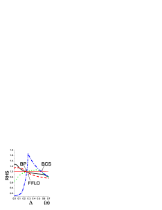
Figure 3: (color online) (a) The right-hand side (R. H. S.) of the gap equation Eq.(8) as a function of $\Delta$ with different values of $q$. $q=0$ for the dash-dotted line, $q=0.175k_{\text{Fa}}$ for the dotted line, $q=0.255k_{\text{Fa}}$ for the solid line and $q=0.35k_{\text{Fa}}$ for the dash line. (b) The solutions of the gap equation Eq.(8), $\Delta_{q}$, as a function of $q$. Both figures are plotted for the chemical potential $\mu$ fixed at $E_{\text{Fa}}$, $\Delta k_{\text{F}}=0.41k_{\text{Fa}}$ and $V=8\times 10^{-8}E_{\text{Fa}}$. The unit of $q$ is $k_{\text{Fa}}$, and the unit of $\Delta$, $\mu$ and $V$ is taken as $E_{\text{Fa}}=\hbar^{2}k_{\text{Fa}}^{2}/(2m_{1})$ with $\hbar^{2}/(2m_{1})$ setting as unity.

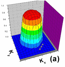
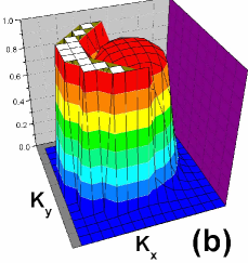
Figure 4: (color online) A illustration of the distribution of atoms(a) and the distribution of molecules(b) in the FFLO state. Here $\Delta k_{\text{F}}=0.41k_{\text{Fa}}$, $q=0.255k_{\text{Fa}}$, and $V=8\times 10^{-8}E_{\text{Fa}}$.

In the Fig.3(a) we plot the right-hand side of the gap equation Eq.(8) as a function of $\Delta_{q}$ with different values of $q$, from which we can know all the possible solutions to the gap equation. We find that the equation for $\Delta_{0}$ has two solutions. The one of large $\Delta$ is the BCS solution, where Cooper pairs are formed around $k_{\text{F}}=[(k^{3}_{\text{Fa}}+k^{3}_{\text{Fm}})/2]^{1/3}$ and the excitation spectrums are all gapped; and another of small $\Delta$ corresponds to the breached-pair state. The energy of the breached-pair state has been extensively studied before for similar modelBP and will not be repeated here. The curves with small $q$, such as $q=0.175k_{\text{Fa}}$, are similar to the curve with $q=0$. However, as $q$ increases the gap equation has only one solution at small $\Delta$, which corresponds to the FFLO states. The values of $\Delta_{q}$ are obtained numerically for different $q$, and shown in Fig.3(b). The small $\Delta$ solutions, including the breached-pair state and the FFLO states, are all characterized by the existence of the deparing region, which can be found from Fig.4 where the particle populations of a typical FFLO state are shown.

In the FFLO state, the center of Fermi sphere moves to ${\bf q}$. The atoms pair with molecules at the small momentum side of the Fermi sphere, while the pairs at the high-momentum side will break. In this way, the FFLO states find a proper balance between lowering the interaction energy and not costing too much kinetic energy, and the nonzero momentum carried by the pairs can be cancelled out by the depaired normal molecules, producing an energetic stable FFLO state with the total momentum $Q$ vanishing. We calculate the total momentum of the FFLO states for different values of $q$ and find stable state exists for large $\Delta k_{\text{F}}$, such as $\Delta k_{\text{F}}=0.41k_{\text{Fa}}$ as shown in Fig. 5(a), and in Fig. 5(b) we also compare the energy of two FFLO states with the BCS state, and find the FFLO state will dominate over the BCS state with the increase of $\Delta k_{\text{F}}$.

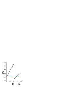
Figure 5: (color online)(a) The momentum per particle $Q/N$ of the FFLO states for different values of $q$. $\Delta k_{\text{F}}$ is fixed at $0.41k_{\text{Fa}}$. (b) The free energy per particle $F=E/N-\mu$ as a function of $\Delta k_{\text{F}}$ for BCS state (dotted line) and the FFLO states with $q=0.255k_{\text{Fa}}$(solid line) and $q=0.30k_{\text{Fa}}$(dash line). We change $\Delta k_{\text{F}}$ by tuning $E_{\text{b}}$. Both figures are plotted for $V=8\times 10^{-8}E_{\text{Fa}}$. The units of $q$, $Q$ and $\Delta k_{\text{F}}$ is $k_{\text{Fa}}$ and the unit of $F$ is $E_{\text{Fa}}$.

Remark. Although we have demonstrated the existence of non-BCS type pairing state in certain region, the phase diagram of this system in the full parameter region is much richer. With the increase of $E_{\text{b}}$, the system will enter a pure atomic phase, the atom-molecule pairing will be replaced by the $p$-wave pairing between fermionic atoms. Provided that the electric moments of these heteronuclear molecules are polarized by an external electric field, the direct dipole-dipole interactions between molecules can not be neglected, and it will lead to the pairing between moleculesdipole . The competition between these different superfluid orders will manifest itself in quantum phase transitions, and more fruitful physics is expected from the interplay of these phases, which will be a subject for further inverstigations.

The authors would like to thank Professor C. N. Yang for encouragement and valuable support, and we thank L. Chang, T. L. Ho, F. Zhou, Z. Z. Chen, R. Lü and M. Zhang for helpful discussions, and we would like to thank Q. Zhou for critical reading the manuscript. This work is supported by NSF China (No. 10247002 and 10404015).

References

- (1) M. Greiner et al., Nature (London) 426, 537 (2003); S. Jochim et al., Science 302, 2101 (2003) and M. W. Zwierlein et al., Phys. Rev. Lett. 91, 250401 (2003).
- (2) C. A. Regal, M. Greiner, and D. S. Jin, Phys. Rev. Lett. 92, 040403 (2004), C. Chin et al., Science 305 1128 (2004).
- (3) M. Greiner, C. A. Regal, and D. S. Jin, Phys. Rev. Lett. 94, 070403 (2005), M. Bartenstein et al., Phys. Rev. Lett. 92, 203201 (2004).
- (4) C.A. Stan, M.W. Zwierlein, C.H. Schunck, S.M.F. Raupach, and W. Ketterle, Phys. Rev. Lett. 93, 143001 (2004).
- (5) S. Inouye, J. Goldwin, M. L. Olsen, C. Ticknor, J. L. Bohn, and D. S. Jin, Phys. Rev. Lett. 93, 183201 (2004).
- (6) P. Fulde and R. A. Ferrell, Phys. Rev. 135 A550 (1964).
- (7) A. I. Larkin and Yu. N. Ovchinnikov, Sov. Phys. JETP 20, 762 (1965).
- (8) A. Bianchi et al., Phys. Rev. Lett. 91, 187004 (2003); and K. Kakuyanagi et al., Phys. Rev. Lett. 94, 047602 (2005).
- (9) R. Casalbuoni and G. Nardulli, Rev. Mod. Phys. 76, 263 (2004).
- (10) R. Combescot, Europhys.Lett. 55, 150 (2001).
- (11) T. Mizushima, K. Machida, and M. Ichioka, Phys. Rev. Lett. 94, 060404 (2005).
- (12) W. V. Liu and F. Wilczek, Phys. Rev. Lett. 90, 047002 (2003); E. Gubankova, W. V. Liu, and F. Wilczek, Phys. Rev. Lett. 91, 032001 (2003), M. M. Forbes et al., Phys. Rev. Lett. 94, 017001 (2005); and S. T. Wu, and S. K. Yip, Phys. Rev. A 67, 053603 (2003).
- (13) H. Müther and A. Sedrakian, Phys. Rev. Lett. 88, 252503 (2002); A. Sedrakian et al., cond-mat/0504511.
- (14) S. Takada and T. Izuyama, Prog. Theor. Phys. 41, 634 (1969).
- (15) For instance, L. Viverit, C. J. Pethick, and H. Smith, Phys. Rev. A 61, 053605 (2000); M. J. Bijlsma, B. A. Heringa, and H. T. C. Stoof, Phys. Rev. A 61, 053601 (2000); and H. Pu et al., Phys. Rev. Lett. 88, 070408 (2002).
- (16) M. Holland et al, Phys. Rev. Lett. 87, 120406 (2001); S. J. J. M. F. Kokkelmans and M. J. Holland, Phys. Rev. Lett. 89, 180401 (2002).
- (17) S. Powell, S. Sachdev and H. P. Buchler, cond-mat/0502299.
- (18) D. B. M. Dickerscheid et al., cond-mat/0502328.
- (19) P. R. Feynman, Statistical Mechanisc p270 (Addison Wesley, Massachusetts, 1998).
- (20) M. A. Baranov, L. Dobrek, and M. Lewenstein, Phys. Rev. Lett. 92, 250403 (2004); L. You and M. Marinescu, Phys. Rev. A 60, 2324 (1999).