Least action principle for envelope functions in abrupt heterostructures

Abstract

We apply the envelope function approach to abrupt heterostructures starting with the least action principle for the microscopic wave function. The interface is treated nonperturbatively, and our approach is applicable to mismatched heterostructure. We obtain the interface connection rules for the multiband envelope function and the short-range interface terms which consist of two physically distinct contributions. The first one depends only on the structure of the interface, and the second one is completely determined by the bulk parameters. We discover new structure inversion asymmetry terms and new magnetic energy terms important in spintronic applications.

The envelope function method is a powerful tool which has been widely used to describe and predict various effects in semiconductors. It is normally applicable to materials with translation invariance (allowing for the expansion of the wave function into Bloch functions) and to slowly varying potentials. There are two competing approaches to extending this method to abrupt heterostructures foreman_prl taking into account interface–related effects. The first one is to impose appropriate boundary conditions (interface connection rules) on the envelope wave function at the interface bc ; gbc ; lagr1 ; ivkamros . Another possibility is deriving the exact envelope function differential equations which are valid near the interface and which contain the iterface–related terms foremanburt ; volkov . The second approach is more detailed, and it requires a lot more information on the microscopic structure of the interface. Up to now, it has only been applied to the lattice–matched heterostructures where the interface is a weak perturbation. In this case, it has been shown foreman_prl that connection rules and differential equations are equally valid representations of the interface behavior.

It is the aim of this letter to present an extension of the envelope function method which treats the interface nonperturbatively, and which is applicable to mismatched heterostructures. It turns out that the best approach to the problem is via the Lagrangian variational principle which encodes the Schrödinger equation. The advantage of this method is that both the Hamiltonian and the boundary conditions at the interface are contained in the averaged variational functional. The resulting ${\bm{k}}\cdot{\bm{p}}$ heterostructure Hamiltonian coincides with the ordinary ${\bm{k}}\cdot{\bm{p}}$ Hamiltonians on two sides of the interface. In addition, it contains short–range interface (SRI) terms which are the main object of our study. We show that the SRI terms consist of two physically distinct contributions. The first one is represented by the Hermitian interface matrix. Its components are directly connected to the parameters of boundary conditions for the envelope functions bc and determined by the microscopic structure of the interface. The second contribution is completely determined by the bulk parameters of the materials. It includes new structure inversion asymmetry (SIA) terms and new SRI magnetic terms that are additional to the well known Rashba SIA terms and to the macroscopic magnetic terms, respectively. Taking them into account is important for various mechanisms of spin polarization, spin filtering and spin manipulation that play a key role in semiconductor spintronic applications spintronic .

In this letter we consider a model of a semiconductor heterostructure made of two homogeneous semiconductor layers $A$ and $B$ of characteristic length $L$. The layers are joined by a thin boundary region $\Pi$ of the width $d\approx a_{0}\ll L$ (see Fig. 1), where $a_{0}$ is the lattice constant. We work in the single electron approximation, and we denote by $U(\bm{r})$ the effective potential for electrons. $U(\bm{r})$ coincides with periodic crystal potentials $U_{A,B}(\bm{r})$ inside the bulk–like regions $A$ and $B$, respectively.

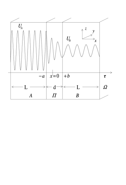
Figure 1: Sketch of the planar heterointerface between $A$ and $B$ semiconductor layers. $\Pi$ denotes the boundary region. $U_{A}$($U_{B}$) is the crystal potential in $A$($B$).

We start with the microscopic Lagrangian variational principle which encodes the stationary single electron Schrödinger equation. The corresponding Lagrangian density is of the form,

$${\cal L}(\Phi^{*},\Phi) = (E-U(\bm{r}))|\Phi({\bm{r}})|^{2}-\frac{\hbar^{2}}{2m_{0}}|\nabla\Phi|^{2}\,.$$ (1)

Here $m_{0}$ is the free electron mass and $\Phi$ is the microscopic spinor wave function. To simplify the presentation we first neglect the spin-orbit terms in Eq. (1). The variational principle reads,

$$\delta{\cal S} = \delta\int_{\Omega}{\bm{d}}^{3}{\bm{r}}{\cal L}(\Phi^{*},\Phi)=0\,,$$ (2)

where variations $\delta\Phi$ and $\delta\Phi^{*}$ are independent of each other and vanish at the outer boundaries of the integration region $\Omega=A+\Pi+B$. The variational principle implies the microscopic Schrödinger equation $\hat{H}_{\rm micro}{\Phi}({\bm{r}})=E{\Phi}({\bm{r}})$ with the microscopic Hamiltonian $\hat{H}_{\rm micro}=({\hat{p}^{2}}/{2m_{0}}+U(\bm{r}))$, where $\hat{\bm{p}}=-i\hbar{\bm{\nabla}}$ is the momentum operator. The microscopic probability flux density ${\bm{j}}=({\Phi}^{*}({\bm{r}})\hat{\bm{p}}{\Phi}({\bm{r}})+\hat{\bm{p}}^{*}{\Phi}^{*}({\bm{r}}){\Phi}({\bm{r}}))/2m_{0}$ is conserved: ${\bm{\nabla}}{\bm{j}}=0$, the microscopic wave function $\Phi$ is continuous everywhere in the heterostructure.

It is our aim to pass from the description in terms of the microscopic wave function $\Phi$ to the envelope function approximation. To this end, we use expansions ${\Phi({\bm{r}})}=\sum_{n=1}^{N_{A,B}}\Psi_{n}^{A,B}({\bm{r}})u_{n}^{A,B}$ within $A$ and $B$. Here $u_{n}^{A,B}$, $n=N_{A,B}$ are the Bloch functions at extremum points of the bulk energy band structure. The $N_{A,B}$ component envelope functions $\Psi_{n}^{A,B}({\bm{r}})$ are smooth in the $A$ and $B$ regions where they satisfy matrix Schrödinger equations $\hat{H}^{A,B}(\hat{\bm{k}}){\Psi}^{A,B}({\bm{r}})=E{\Psi}^{A,B}({\bm{r}})$. Here $\hat{H}^{A,B}=\hat{C}+\hbar\hat{B}^{\mu}\hat{k}_{\mu}+\hbar^{2}\hat{D}^{\mu\,\nu}\hat{k}_{\mu}\hat{k}_{\nu}$ are the standard ${\bm{k}}\cdot{\bm{p}}$ Hamiltonians including the terms up to the second order in the wave vector operator $\hat{\bm{k}}=-i{\bm{\nabla}}$. The matrices $\hat{C}$, $\hat{B}^{\mu}$ and $\hat{D}^{\mu\,\nu}$ ($\mu\,,\nu=x,y,z$) are Hermitian $N_{A,B}\times N_{A,B}$ tensors of rank $0$,$1$, and $2$, respectively. The Hamiltonians $\hat{H}^{A,B}$ give a direct description of the $N_{A,B}$ basic bands as well as the contributions of the remote bands in the second order of perturbation theory bir . Note that symmetry of the materials, the number of basic bands in the ${\bm{k}}\cdot{\bm{p}}$ approximation can be different on two sides of the interface. Moreover, parameters of bulk Hamiltonians $\hat{H}^{A,B}$ can vary significantly across the interface, so as it cannot be treated as a weak perturbation of the bulk problem.

We fix once and for all the basic functions $u^{A,B}$ in $A$ and $B$, and we derive the ${\bm{k}}\cdot{\bm{p}}$ version of Lagrangian variational principle. The result has the form $\delta{\cal S}_{\rm kp}=\delta{\cal S}_{A}+\delta{\cal S}_{B}+\delta{\cal S}_{\rm sur}=0$, and it contains $\tilde{N}=N_{A}+N_{B}$ independent variations of the envelope wave functions $\delta\Psi_{n}^{A},\delta\Psi_{n}^{B}$. Here $\delta{\cal S}_{A,B}=\int_{{{A,B}}}{\bm{d}}^{3}{\bm{r}}{\cal L}({\Phi}^{*},{\Phi})=\int_{{{A,B}}}{\bm{d}}^{3}{\bm{r}}{\cal L}_{A,B}({\Psi}^{*},{\Psi})$ and $\delta{\cal S}_{\rm sur}=\delta\int_{{\bm{\Pi}}}{\bm{d}}^{3}{\bm{r}}\delta(x){\cal L}_{\rm sur}$, where $\delta(x)$ is the Dirac delta–function. The bulk multiband Lagrangian densities ${\cal L}_{A,B}$ are obtained from the microscopic Lagrangian by averaging over the unit cells in $A$ and $B$, respectively. They have the form:

$${\cal L}({\Psi}^{*},{\Psi})=E|\Psi|^{2}-\Psi^{*}\hat{C}\Psi-\frac{\hbar^{2}}{2}{\nabla}_{\mu}\Psi^{*}\hat{A}^{\,\mu\,\nu}{\nabla}_{\nu}\Psi$$ (3)

$$-\frac{i\hbar}{2}\left({\bm{\nabla}}\Psi^{*}\hat{\bm{B}}\Psi-\Psi^{*}\hat{\bm{B}}{\bm{\nabla}}\Psi\right)+\frac{\hbar^{2}}{2}{\bm{\nabla}}\Psi^{*}\cdot[\hat{\bm{K}}\times{\bm{\nabla}}\Psi]\,.$$

Here $\hat{A}^{\mu\,\nu}=\hat{D}^{\mu\,\nu}+\hat{D}^{\nu\,\mu}$, $\hat{K}^{\eta}=\epsilon_{\eta\mu\nu}\hat{D}^{\mu\,\nu}$, $\eta,\mu,\nu=x,y,z$ and $\epsilon_{xyz}$ is Levi-Civita anti-symmetric tensor. The surface Lagrangian is nonlocal and it can be written as

$${\cal L}_{\rm sur}=\tilde{\Psi}^{*}\hat{T}_{\rm sur}\tilde{\Psi}\,,\quad\hat{T}_{\rm sur}=\frac{\hbar^{2}}{2m_{0}}\left(\begin{array}[]{cc}\hat{t}^{A}/a&\hat{t}/d\\ \hat{t}^{*}/d&\hat{t}^{B}/b\end{array}\right)\,,$$ (4)

where

$\tilde{\Psi}=\left(\begin{array}[]{c}\Psi^{A}({\bm{\rho}},x-a)\\ \Psi^{B}({\bm{\rho}},x+b)\end{array}\right)$, with ${\bm{\rho}}=(y,z)$, and $d=a+b$ (see Fig. 1). The energy independent hermitian $\tilde{N}\times\tilde{N}$ interface matrix $\hat{T}_{\rm sur}$ depends on the symmetry of both bulk materials and of the interface. It can be constructed by using the method of the invariants bir or calculated directly via the microscopic modeling of the potential $U(r)$ in the interface region $\Pi$ (the details will be presented elsewhere).

The effective Lagrangians ${\cal L}_{A,B}$ together with ${\cal L}_{\rm sur}$ contain all the relevant information about the bulk and interface properties of the heterostructure. Application of the least action principle $\delta{\cal S}_{\rm kp}=0$ generates the Schrödinger equation $\hat{H}_{AB}\tilde{\Psi}=E\tilde{\Psi}$ with the complete heterostructure ${\bm{k}}\cdot{\bm{p}}$ Hamiltonian $\hat{H}_{AB}$ and the general boundary conditions (GBC) to be imposed on $\Psi^{a}=\Psi^{A}({\bm{\rho}},-a)$ and $\Psi^{b}=\Psi^{B}({\bm{\rho}},b)$. The GBC (see bc ) can be written as $\left(\begin{array}[]{c}i\hat{V}_{\tau}\Psi^{a}\\ -i\hat{V}_{\tau}\Psi^{b}\end{array}\right)={\displaystyle{\frac{2\hat{T}_{\rm sur}}{\hbar}}}\left(\begin{array}[]{c}\Psi^{a}\\ \Psi^{b}\end{array}\right)$ or as $\left(\begin{array}[]{c}\Psi^{a}\\ i\hat{V}_{\tau}\Psi^{a}\end{array}\right)=\hat{T}_{\rm tr}\left(\begin{array}[]{c}\Psi^{b}\\ i\hat{V}_{\tau}\Psi^{b}\end{array}\right)$, where the components of the $2N_{A}\times 2N_{B}$ transfer matrix $\hat{T}_{\rm tr}$ (see bc ; gbc ) can be readily expressed via the components of the surface matrix $\hat{T}_{\rm sur}$ (see also balian ). Here ${\bm{\tau}}$ is the normal vector to the interface, $\hat{V}_{\tau}={\bm{\tau}}\cdot\hat{\bm{V}}$, and the envelope velocity operator $\hat{\bm{V}}_{nm}\Psi_{m}={2i}/{\hbar}({\partial{\cal L}}/{\partial{\bm{\nabla}}\Psi^{*}_{n}})$ can be written explicitly as

$$\hat{\bm{V}}=\hat{\bm{B}}+\hbar\frac{\partial\hat{A}^{\mu\nu}\{\hat{k}_{\mu}\hat{k}_{\nu}\}}{\partial{\bm{k}}}-\hbar\left[\hat{\bm{K}}\times\hat{\bm{k}}\right]\,.$$ (5)

The last term is new in comparison to bc . The corresponding extra term in the envelope flux density ${\bm{J}}({\bm{r}})={1}/{2}\left({\Psi}_{n}^{*}\hat{\bm{V}}_{nm}{\Psi_{m}}+{\Psi_{n}}(\hat{\bm{V}}_{nm}{\Psi_{m}})^{*}\right)$ is proportional to ${\bm{\nabla}}\times(\Psi^{*}\hat{\bm{K}}\Psi)$ and does not alter the continuity property ${\bm{\nabla}}\cdot{\bm{J}}=0$. It is straightforward to verify that $J^{\alpha\,\beta}_{\tau}={\bm{\tau}}\cdot{\bm{J}}^{\alpha\,\beta}({\bm{r}})={\rm const}$, where $\alpha$ and $\beta$ label two functions $\Psi_{\alpha}$ and $\Psi_{\beta}$ satisfying the same GBC (see Ref. bc ). This ensures that the heterostructure ${\bm{k}}\cdot{\bm{p}}$ Hamiltonian $\hat{H}_{AB}$ is self-adjoint. It has the form:

$$\hat{H}_{AB}=\left(\begin{array}[]{cc}\hat{H}^{A}_{h}+\delta(x)\hat{H}_{\rm sri}^{A}&\delta(x)\hat{H}_{\rm sri}^{AB}\\ \delta(x)\hat{H}_{\rm sri}^{BA}&\hat{H}^{B}_{h}+\delta(x)\hat{H}_{\rm sri}^{B}\end{array}\right)\,,$$ (8)

where $\hat{H}^{A}_{h}=\Theta(-x)\hat{H}^{A}({\bm{\rho}},x-a)$, $\hat{H}^{B}_{h}=\Theta(x)\hat{H}^{A}({\bm{\rho}},x+b)$, $\Theta(x)$ is the Heaviside step function and

$$\hat{H}_{\rm sri}^{A}=\frac{\hbar}{2}\left(i\hat{V}_{\tau}^{A}+\frac{\hbar}{m_{0}a}\hat{t}_{a}\right)\,,\quad H_{\rm sri}^{AB}=\frac{\hbar^{2}}{2m_{0}d}\hat{t}\,,$$ (9)

$$\hat{H}_{\rm sri}^{B}=\frac{\hbar}{2}\left(-i\hat{V}_{\tau}^{B}+\frac{\hbar}{m_{0}b}\hat{t}_{b}\right)\,,\quad H_{\rm sri}^{BA}=\frac{\hbar^{2}}{2m_{0}d}\hat{t}^{*}\,.$$

We see that there are two physically distinct contributions to the short–range interface (SRI) terms of the Hamiltonian $\hat{H}_{AB}$. The first one arises from the nonlocal surface Lagrangian ${\cal L}_{\rm sur}$ and it depends on the properties of the interface via the energy independent parameters of the GBC. The other contribution comes from the velocity operator $\hat{V}_{\tau}$. It is entirely determined by the bulk parameters and it arises from the nonvanishing variation of the bulk Lagrangians ${\cal L}_{A,B}$ at the interface. The important feature of this contribution is the presence of the asymmetric $\hat{\bm{K}}$ term. In homogeneous semiconductors the asymmetric $\hat{\bm{K}}$ term does not contribute to $\hat{H}$ in the absence of external fields (see lut ). Examples below demonstrate that the $\hat{\bm{K}}$ terms in the Lagrangian of Eq. (3) and in the velocity operator of Eq. (5) become important if the symmetry is broken due to the presence of external fields or asymmetric interfaces. To emphasize this point we neglect effects of bulk inversion asymmetry.

As a first example, we consider the effective mass Hamiltonian $\hat{H}(\Gamma_{6})=E_{c}+{\hbar^{2}\hat{k}^{2}}/{2m}$ for the spinor envelope function $\Psi_{\alpha}$ ($\alpha=\pm 1/2$), where $E_{c}$ is the bottom of the conduction band and $m$ is the effective mass. Following our method we introduce the effective mass Lagrangian density

$${\cal L}=(E-E_{c})|\Psi|^{2}-\frac{\hbar^{2}}{2m}|\nabla\Psi({\bm{r}})|^{2}+{\cal L}_{\rm SIA}\,,$$ (10)

which contains the asymmetric term

$${\cal L}_{\rm SIA}(\Gamma_{6})=-\frac{i\hbar^{2}}{4m_{0}}\tilde{g}{\bm{\nabla}}\Psi^{*}[{\bm{\sigma}}\times{\bm{\nabla}}\Psi]\,$$ (11)

obtained with ${\bm{K}}(\Gamma_{6})=-(i\tilde{g}/2m_{0}){\bm{\sigma}}$, where $\sigma_{x}$, $\sigma_{y}$, $\sigma_{z}$ are Pauli matrices, and $\tilde{g}=g_{0}-g$ is the difference between free electron and effective electron $g$ factors. Note that $\tilde{g}\neq 0$ only if the spin-orbit splitting $\Delta$ of the valence band or $\Delta^{c}$ of the remote conduction band is taken into account. We discover now that it is this asymmetric term ${\cal L}_{\rm SIA}(\Gamma_{6})$ (missing in Refs. lagr1 ; lagr ) that induces the spin dependence of the velocity operator $\hat{\bm{V}}=(\hbar/m)\hat{\bm{k}}-({i\hbar}\tilde{g}/2{m_{0}})[{\bm{\sigma}}\times\hat{\bm{k}}]$ and thus the spin dependence of the standard boundary conditions $\Psi={\rm const}$, $\hat{V}_{\tau}\Psi={\rm const}$ at the interface (see vasko ; pfeffer ). The short-range interface SIA term in the heterostructure Hamiltonian $\hat{H}_{AB}$ of Eq. (8) also results from ${\cal L}_{\rm SIA}(\Gamma_{6})$. Moreover, exactly this term ${\cal L}_{\rm SIA}(\Gamma_{6})$ produces the magnetic energy term $-{1}/{2}\mu_{B}\tilde{g}({\bm{\sigma}}{\bm{H}})$ additional to the free electron magnetic energy ${1}/{2}\mu_{B}g_{0}({\bm{\sigma}}\,{\bm{H}})$ in the bulk semiconductor in external magnetic field ${\bm{H}}$. Here $\mu_{B}$ is the Bohr magneton. Next, it can be shown that the macroscopic SIA term $\hat{H}^{\rm so}=\alpha_{R}[{\bm{\sigma}}\times\hat{\bm{k}}]{\bm{\tau}}$, postulated by Rashba rashba for the asymmetric $2D$ structure, is generated by the term ${\cal L}_{\rm SIA}(\Gamma_{6})$. For this the dependence of $g$ on the potential $V=-|e|{\cal E}x$ should be taken into consideration, where the average electric field ${\bm{E}}={\cal E}{\bm{\tau}}$ characterizes the macroscopic asymmetry. In the eight band model for cubic semiconductors $g=g_{0}-g_{r}-2E_{p}\Delta/3(E_{g}-V)(E_{g}-V+\Delta)$, where $E_{p}$ is Kane energy, $E_{g}$ is a band gap and $g_{r}$ is a correction from remote bands, and the effective Rashba constant is $\alpha_{R}\propto\left.\partial g/\partial x\right|_{x=0}\propto\Delta$. Using the expression for $g$ in the 14 band model one finds that the correction to $\alpha_{R}$ is proportional to $\Delta^{c}$.

Another useful example is provided by the degenerate valence band at the $\Gamma$ point described by the envelope Hamiltonians obtained in lut . We consider two cases of $\Delta=0$ and $\Delta\rightarrow\infty$. The remarkable property of the respective envelope Lagrangians obtained according to Eq. (3) is the existence of the asymmetric term with ${\bm{K}}(\Gamma_{15})=-i(1+3\kappa)/m_{0}{\bm{I}}$ even in the case $\Delta=0$:

$${\cal L}_{\rm SIA}(\Gamma_{15})=-\frac{i\hbar^{2}}{2m_{0}}(1+3\kappa){\bm{\nabla}}\Psi_{\alpha}^{*}[{\bm{I}}\times{\bm{\nabla}}\Psi_{\alpha}]\,.$$ (12)

Here $\kappa$ is the magnetic Luttinger constant, $\hat{\bm{I}}$ is the internal angular momentum operator ($I=1$) and $\Psi_{\alpha}$, $\alpha=0,\pm 1$, is the 3 component envelope function. The SIA component of the velocity operator $\hat{\bm{V}}_{\rm so}={i\hbar}(1+3\kappa)/{m_{0}}[{\bm{I}}\times{\bm{k}}]$ induces a new short range SIA term in the heterostructure Hamiltonian for the $\Gamma_{15}$ holes as well as the ${\bm{I}}$-dependent boundary conditions. This leads to the splitting of the heavy hole subband in asymmetric structures mediated by the interaction with light hole states. Note that it is this asymmetric term ${\cal L}_{\rm SIA}(\Gamma_{15})$ which is responsible for the magnetic energy term $\propto\mu_{B}(1+3\kappa)({\bm{I}}{\bm{H}})$ in the bulk Hamiltonian of Ref. lut .

In the case of $\Delta\rightarrow\infty$, the top of valence band is four-fold degenerate corresponding to the $J=3/2$ subspace of the total internal momentum ${\bm{J}}={\bm{I}}+1/2{\bm{\sigma}}$. We obtain the asymmetric term in the envelope Lagrangian with ${\bm{K}}(\Gamma_{8})=-i(2/3+2\kappa)/m_{0}{\bm{J}}-iq/m_{0}{\bm{F}}$, where $q$ is cubically anisotropic magnetic Luttinger constant and ${\bm{F}}=(F_{x},F_{y},F_{z})\equiv(J_{x}^{3},J_{y}^{3},J_{z}^{3})$:

$${\cal L}_{\rm SIA}(\Gamma_{8})=\frac{\hbar^{2}}{2}{\bm{\nabla}}\Psi_{\alpha}^{*}[{\bm{K}}(\Gamma_{8})\times{\bm{\nabla}}\Psi_{\alpha}]\,.$$ (13)

Here $\Psi_{\alpha}$, $\alpha=\pm 3/2,\pm 1/2$, is the 4 component envelope wave function. The SIA component of the velocity operator $\hat{\bm{V}}_{\rm so}={i\hbar}/m_{0}((2/3+2\kappa)[{\bm{J}}\times{\bm{k}}]+q[{\bm{F}}\times{\bm{k}}])$ produces a new short range SIA term in the heterostructure Hamiltonian as well as the asymmetric contribution to the boundary conditions of the $\Gamma_{8}$ holes (see pfeffer ; foreman ). The very same asymmetric term ${\cal L}_{\rm SIA}(\Gamma_{8})$ induces the magnetic energy terms $\propto({\bm{J}}{\bm{H}})$ and $\propto q({\bm{F}}{\bm{H}})$ in the bulk Hamiltonian of Ref. lut as well as the macroscopic SIA term $H^{\rm so}_{8v}=\beta_{1}[{\bm{J}}\times{\bm{k}}]{\bm{E}}+\beta_{2}[{\bm{F}}\times{\bm{k}}]{\bm{E}}$ postulated recently in Ref. winkler . The cubically anisotropic constant $q$ and, consequently, $\beta_{2}$ are proportional to $\Delta^{c}$ and usually small. Considering the dependence of $\kappa=\kappa_{r}+E_{p}/6(E_{g}+V)$ on $V=-|e|{\cal E}x$, where $\kappa_{r}$ is the contribution from remote bands, we are able to derive for the first time the effective SIA constant $\beta_{1}$ for the $\Gamma_{8}$ valence band:

$$\beta_{1}=\frac{|e|\hbar^{2}}{6m_{0}}\frac{E_{p}}{E_{g}^{2}}\,.$$ (14)

We found that in contrast to the Rashba constant, $\beta_{1}$ is not proportional to the spin–orbit splittings $\Delta$ or $\Delta_{c}$.

The short–range SIA contribution to the zero field splitting becomes more pronounced in the case of the interface between very dissimilar materials. The general Hamiltonian $\hat{H}_{AB}$ of Eqs. (8,Least action principle for envelope functions in abrupt heterostructures) enables to describe, for example, the interface coupling between $\Gamma_{6}$ electrons and $\Gamma_{8}$ holes and the SIA effects in type II and type III quantum wells, and to take into consideration the microscopic asymmetry caused by the nonequivalence of two opposite interfaces (see as ).

Finally, the developed approach reveals a new short–range magnetic energy term in the heterostructure Hamiltonian $\hat{H}_{AB}$ in the presence of the in-plane external magnetic field. Indeed, choosing ${\bm{H}}\parallel{\bm{z}}$ we obtain the new term in the velocity operators $V_{\tau}\Psi$ proportional to $Hx(\hat{K}_{z}\Psi)$. In small fields this term can be treated as a perturbation. The short-range contribution to the Zeeman energy is proportional to the sum of the discontinuities of $(\Psi^{*}\hat{K}_{z}\Psi)$ at the interfaces. Unlike the zero field splitting, this interface magnetic energy contribution is present even in completely symmetric $2D$ structures as well as in spherical dots (see so ).

In conclusion, the variational least action principle allows to consistently extend the envelope function approach to the heterostructures with abrupt interfaces. The SRI terms in the heterostructure Hamiltonian $\hat{H}_{AB}$ and the GBC are equally valid representation of the interface properties and can be written for any interface between dissimilar materials including the case $N_{A}\neq N_{B}$. For lattice-matched heterostructures ($N_{A}=N_{B}=N$) the obtained $\hat{H}_{AB}$ allows direct comparison with previously derived Hamiltonians foremanburt ; volkov ; foreman . The discretization of $\hat{H}_{AB}$ for numerical calculations is straightforward and requires no additional symmetrization. All macroscopic and short-range interface SIA terms as well as the magnetic energy terms in $\hat{H}_{AB}$ originate from the asymmetric term ${\cal L}_{\rm SIA}$ in the bulk envelope Lagrangian.

We are grateful to R. Suris for attracting our attention to the importance of the variational principle for boundary condition problems. A.V. Rodina acknowledges the support from the Swiss National Science Foundation.

References

- (1) B. A. Foreman, Phys. Rev. Lett. 80, 3823 (1998).
- (2) A. V. Rodina, A. Yu. Alekseev, Al. L. Efros, M. Rosen, and B. K. Meyer, Phys. Rev. B 65, 125302 (2002).
- (3) I. V. Tokatly, A. G. Tsibizov, and A. A. Gorbatsevich, Phys. Rev. B 65, 165328 (2002); M. V. Kisin, B. L. Gelmont, and S. Luryi, Phys. Rev. B 58, 4605 (1998).
- (4) Smadar de-Leon, B. Laikhtman, and L. D. Shvartsman, J. Phys.: Condens. Matter 10, 8715 (1998).
- (5) E. L. Ivchenko, A. Yu. Kaminski, and U. Rössler, Phys. Rev. B 54, 5852 (1996).
- (6) M. G. Burt, J. Phys. Condens. Matter 4, 6651 (1992); B. A. Foreman, Phys. Rev. B 54, 1909 (1996); B. A. Foreman, Phys. Rev. Lett. 81, 425 (1998).
- (7) E. E. Takhtamirov and V. A. Volkov, Semicond. Sci. Technol. 12, 77 (1997); E. E. Takhtamirov and V. A. Volkov, Zh. Eksp. Teor. Fiz. 116, 1843 (1999) [JETP89, 1000 (1999)].
- (8) L. P. Rokhinson, V. Larkina, Y. B. Lyanda-Geller, L.N.Pfeiffer, and K.W. West, Phys. Rev. Lett. 93, 146601 (2004); M. Khodas, A. Shekhter, and A. Finkel’stein, Phys. Rev. Lett. 92, 086602 (2004); E. I. Rashba and Al. L. Efros, Phys. Rev. Lett. 91, 126405 (2003).
- (9) E. I. Ivchenko and G. E. Pikus, Superlattices and Other Heterostucture (Springer, Berlin, 1995).
- (10) R. Balian, D. Bessis, and G. A. Mezincescu, Phys. Rev. B 51, 17624 (1995).
- (11) J. M. Luttinger, Phys. Rev. 102, 1030 (1956).
- (12) F. S.A. Cavalcante, R. N. Costa Filho, J. Ribeiro Filho, C. A. S. de Almeida, and V. N. Freire, Phys. Rev. B 55, 1326 (1997); H. C. Liu, Supperlattice and Microstructures 3, 413 (1987).
- (13) F. T. Vasko, Pis’ma Zh. Eksp. Theor. Fiz. 30, 574 (1979) [JETP Lett. 30, 541 (1979)].
- (14) P. Pfeffer and W. Zawadzki, Phys. Rev. B 59, R5312 (1999); E. A. de Andrada e Silva, G. C. La Rocca, and F. Bassani, Phys. Rev. B 55, 16 293 (1997).
- (15) Yu. A. Bychkov and E. I. Rashba, Pis’ma Zh. Eksp. Theor. Fiz. 39, 66 (1984) [JETP Lett. 39, 78 (1984)].
- (16) B.A. Foreman, Phys. Rev. B 48, R4964 (1993); G. F. Glinskii, K. O. Kravchenko, Fiz. Tverdogo Tela 40, 872 (1998).
- (17) R. Winkler, Phys. Rev. B 62, 4245 (2000).
- (18) T. Reker, H. Im, L. E. Bremme, H. Choi, Y. Chung, P. C. Klipstein, and H. Shtrikman, Phys. Rev. Lett. 88, 056403 (2002); A. V. Platonov, V. P. Kochereshko, E. L. Ivchenko, G. V. Mikhailov, D. R. Yakovlev, M. Keim, W. Ossau, A. Waag, and G. Landwehr, Phys. Rev. Lett. 83, 3546 (1999); J. A. Majewski, P. Vogl, and P. Lugli, in Proceedings of the 25th International Conference on Physics of Semiconductors, Osaka, 2000 (Springer, Berlin, 2001), p.791.
- (19) A. V. Rodina, Al. L. Efros, A. Yu. Alekseev, Phys. Rev. B 67, 155312 (2003).