PERIODIC HOMOGENIZATION FOR INERTIAL PARTICLES

Abstract

We study the problem of homogenization for inertial particles moving in a periodic velocity field, and subject to molecular diffusion. We show that, under appropriate assumptions on the velocity field, the large scale, long time behavior of the inertial particles is governed by an effective diffusion equation for the position variable alone. To achieve this we use a formal multiple scale expansion in the scale parameter. This expansion relies on the hypo-ellipticity of the underlying diffusion. An expression for the diffusivity tensor is found and various of its properties studied. In particular, an expansion in terms of the non-dimensional particle relaxation time $\tau$ (the Stokes number) is shown to co-incide with the known result for passive (non-inertial) tracers in the singular limit $\tau\to 0$. This requires the solution of a singular perturbation problem, achieved by means of a formal multiple scales expansion in $\tau.$ Incompressible and potential fields are studied, as well as fields which are neither, and theoretical findings are supported by numerical simulations.

1 Introduction

Understanding the transport properties of particles moving in fluid flows and subject to molecular diffusion is a problem of great theoretical and practical interest [11, 23]. For the purposes of mathematical analysis, the fluid velocity is assumed to have some statistical or geometrical structure which mimics features of real fluid flows, and yet is such that the resulting equation describing the motion of the particle is amenable to both analysis and efficient numerical investigations. For example the velocity may be assumed steady and periodic in space, or may be assumed to be a Gaussian random field in space–time. This is the problem of turbulent diffusion [7, 23].

It is often the case that the velocity field of interest is active at various length and time scales. Consequently, the equations which govern the particle motion are very hard to analyze directly. In such cases an effective equation which governs the behavior of the particles at long times and large scales compared to those of the fluid velocity is sought. The derivation of such an effective equation is based on multiscale/homogenization techniques [4].

This problem has been studied extensively over the last thirty years for passive tracers, i.e. massless particles. It has been shown that, for periodic or random velocity fields with short range correlations, the particles perform an effective Brownian motion. The covariance matrix of this Brownian motion – the effective diffusivity – is computed through the solution of an auxiliary equation, the cell problem. In the case of steady periodic velocity fields the cell problem is a linear elliptic PDE with periodic coefficients. Various properties of the effective diffusivity have been investigated. In particular, it has been shown that the diffusivity is always enhanced (over bare molecular diffusion) for incompressible flows [12, 23, 29] and always depleted for potential flows [46]. Extensions of the above results to the case where the molecular diffusivity is modelled as colored noise have also been analyzed [5].

However, there are various applications where the particles cannot be modelled as tracers and inertial effects have to be taken into account. The need for adequate modelling and analysis of the motion of inertial particles in various applications in science and engineering has been recognized over the last few years with a number of publications in this direction [8, 10, 38]. As well as bringing important physical features into the problem, the presence of inertia also renders the mathematical study of the resulting equations more delicate. The purpose of the present paper is to study the long time, large scale behavior of inertial particles moving in periodic velocity fields, under the influence of molecular diffusion. Both analytical and numerical techniques are used. From a physical standpoint the main interest in this work is perhaps the enormous enhancement in diffusion which can be introduced through relatively small inertial effects; see section 6. From the mathematical standpoint, the main interest is perhaps (i) the hypo-elliptic structure of the differential operators arising in the multi-scale expansions (section 3) and (ii) the elucidation of the passive tracer limit, from within the inertial particles framework, again by use of multiple scales expansions (section 5).

We consider the diffusive behaviour of trajectories satisfying the equation

$$\tau\ddot{x}=v(x)-\dot{x}+\sigma\dot{\beta},$$ (1)

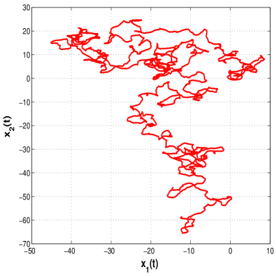
Figure 1: The two components of the solution of (1), (2) with $\tau=\sigma=1.0$.

where $\beta(t)$ is a standard Brownian motion in ${\mathbb{R}}^{d},\,d\geq 1$. In Figure 1 we plot a sample trajectory of (1) with dimension $d=2$, $\tau=1$ and $\sigma=1$; the velocity $v(x)$ is given by the Taylor–Green field:

$$v(x)=\nabla^{\bot}\psi_{TG}(x),\quad\psi_{TG}(x)=\sin(x_{1})\sin(x_{2}).$$ (2)

This figure strongly suggests that the long time behavior of the particles is diffusive. Our goal is to make this type of observation precise. We provide a mathematical formula for the effective diffusivity, and study its properties by a combination of analysis and Monte Carlo simulations. The results raise a number of interesting questions of physical interest, regarding behaviour of the effective diffusivity, and also provide a framework for mathematical analysis to further probe questions of physical interest.

Problems of this type have already been studied in a variety of situations:

1. When $\sigma=0$, $\nabla\cdot U(x)\equiv 0$ and

   $$v(x)=U(x)+\delta\tau U(x)\cdot\nabla U(x)$$ (3)

   we obtain the following model for the motion of a particle in an incompressible steady velocity field [27, 28]:

   $$\ddot{x}=\delta U(x)\cdot\nabla U(x)+\frac{1}{\tau}(U(x)-\dot{x}).$$ (4)

   

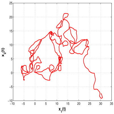
   Figure 2: The two components of the solution of (4), for $U(x)$ given by (2), with $\delta=0.7$ and $\tau=2.0$.

   Here $x(t)$ denotes the particle position and $U(x)$ is the fluid velocity. The parameter $\delta=\frac{\rho_{f}}{\rho_{p}}$ is the ratio between the fluid density and the particle density and $\tau$ denotes the Stokes number. Equation (4) becomes Stokes’ law when $\delta=0$, i.e. when the particles are much denser than the surrounding fluid. The model (4) was analyzed numerically for two dimensional steady incompressible cellular flows by Crisanti et al. [6]. Their numerical experiments showed that for particles slightly denser than the surrounding fluid ($1-\delta\approx 0$ and $\delta<1$), and for $\tau=1$, the particles perform an effective Brownian motion with a well defined diffusion coefficient The term inertial diffusion was introduced to describe this phenomenon. In Figure 2 we present a sample trajectory of (4) with $U(x)$ given by the Taylor Green velocity field (2), for $\tau=2.0$ and $\delta=0.7$. The figure again suggests long time behavior of the particle trajectories which is diffusive. This phenomenon has been observed and analyzed–mostly numerically–by various authors [6, 26, 37, 47, 48]. The range of $\delta$ in which Brownian motion behaviour is observed appears to be connected to the linear stability properties of the equilibria of (4); see the discussion in section 6.

2. When $\sigma=0$, $\nabla\cdot U(x)=0$ and $v(x)=U(x)$ (i.e. $\delta=0$ in (4)) a similar investigation was carried out by Wang et al. in [47] in the case $d=3$. They studied equation (4) numerically for the three–dimensional ABC flow. It is well known that the streamlines of this flow are chaotic [2]. It was exhibited numerically that, for sufficiently small $\tau$, the particles perform Brownian motion. The resulting diffusion coefficient was evaluated numerically and its dependence on $\tau$ was investigated.

3. When $\sigma>0$ and $v(x)=-\nabla V(x)$ it is possible to study the effective behavior of particles moving in a periodic or random potential flow, under the influence of molecular diffusion. This has been addressed by various researchers [15, 22, 31, 35]. In this case the particle motion is governed by the Langevin equation:

   $$\ddot{x}=-\nabla V(x)-\dot{x}+\sigma\dot{\beta},$$ (5)

   where $\beta(t)$ is the standard Brownian motion in $\mathbb{R}^{d}$, $\sigma>0$ and $V(x)$ is a potential which can be either periodic or random. It was shown by Papanicolaou and Varadhan [31] that, for sufficiently smooth random potentials $V(x)$, the particles perform an effective Brownian motion, at long length and time scales, with a nonnegative–definite effective diffusivity. A similar result was proved for periodic potentials in [35] and various refinements were analyzed in [15, 22]. The analysis of equation (5) is greatly simplified by the fact that the explicit form of the invariant distribution associated to the particle position and velocity is known.

4. The problem of averaging for equations of the form (1) with periodic coefficients was studied by Freidlin in [13]. He considered the equation

   $$\tau\ddot{x}=v\left(\frac{x}{\epsilon}\right)-\dot{x}+\sigma\left(\frac{x}{\epsilon}\right)\dot{\beta},$$

   where $v(x),\,\sigma(x)$ are smooth, $1$–periodic functions and the matrix $a(x)=\sigma(x)\sigma(x)^{*}$ is non–degenerate. It was shown in [13] that as $\tau,\,\epsilon$ tend to $0$, the particle position $x$ converges to the solution of a first order SDE with constant coefficients, leading to linear in time mean flow, with superimposed Brownian fluctuations. The averaged coefficients of the limiting SDE depend on how fast $\epsilon$ tends to $0$ relative to $\tau$ and two different cases have to be distinguished.

The purpose of the present paper is to study the long time, large scale behavior of inertial particles satisfying (1) when the velocity field is periodic with period $1$: $v(x+\hat{e}_{j})=v(x),\;\;j=1,\dots,d$ where $\{\hat{e}_{j}\}_{j=1}^{d}$ are the unit vectors in $\mathbb{R}^{d}$. We show, by applying multiscale techniques to the backward Kolmogorov equation associated to (1), that, provided the drift term is centered with respect to the invariant distribution of the stochastic process corresponding to (1), the long time, large scale behavior of the inertial particles is governed by an effective Brownian motion. The effective diffusivity tensor ${\mathcal{K}}$ is computed through the solution of the cell problem which is an equation posed on ${\mathbb{R}}^{d}\times{\mathbb{T}}^{d}$, where ${\mathbb{T}}^{d}$ is the $d$–dimensional unit torus. It is shown that this tensor is nonnegative and that, consequently, the effective dynamics is well–posed. We emphasize that our analysis does not assume any specific structure on the drift term and that, in particular, it is valid for both divergence free as well as potential flows, provided that a centering condition on $v(x)$ is satisfied. However, in the case of potential flows, the effective diffusivity is shown to be depleted, for all Stokes’ numbers, when compared with bare molecular diffusion; this generalizes a known result for passive tracers.

Our theoretical findings are supported by numerical simulations which probe the dependence of the effective diffusivity on parameters such as $\tau$ and, when the velocity field is given by (3), $\delta.$ The equations of motion (1) are solved for the Taylor–Green flow (2) and the long time behavior of the particle trajectories is shown numerically to be that of a Brownian motion. The numerically computed effective diffusivity is compared with the enhancement for passive tracers, i.e. when $\tau=0$, and it is shown that the presence of inertia enhances the diffusivity beyond the enhancement for the passive tracers. The problem is also analyzed through a small $\tau$ expansion of the effective diffusivity. We show that, to leading order in $\tau$, the effective diffusivity is equal to that arising from the homogenization of passive tracers. We also compute the $\mathcal{O}(\tau)$ correction to the effective diffusivity for one dimensional gradient flows of the type (5) and show that it is always negative. Thus, in the one dimensional case and for $\tau$ sufficiently small but positive, the diffusivity is depleted over bare molecular diffusion even further than the depletion which occurs when $\tau=0$.

Here we analyze the problem of homogenization of inertial particles and derive the formula for the effective diffusivity using formal multi–scale calculations. We emphasize that the basic homogenization result derived in this paper can be proved rigorously using techniques from stochastic analysis, in particular the martingale central limit theorem [18]; we refer to [16] for the rigorous proof of the homogenization theorem.

The paper is organized as follows. In section 2 we review homogenization for passive tracers. The derivation of the homogenized equation for the general second order stochastic differential equation (1) with periodic velocity field $v(x)$ is discussed in section 3. Various properties of the effective diffusivity are derived and analyzed in section 4. The homogenization result for the equation (4), subject to molecular diffusion, is also presented there. The small $\tau$ expansion for ${\mathcal{K}}$ is studied in section 5. Numerical experiments for the Taylor–Green flow are presented in section 6. Section 7 contains our conclusions. Finally, some technical results which are needed for the rigorous justification of the multi–scale method employed in this paper are proved in the appendix.

2 Homogenization for Passive Tracers

In this section we review the homogenization result for passive tracers – i.e. massless particles – advected by a velocity field $v(x)$ and subject to molecular diffusion:

$$\dot{x}=v(x)+\sigma\dot{\beta}.$$ (6)

We do this in order to emphasize the structural similarities between this case and the inertial case (1) which is the focus of the paper.

The velocity field $v(x)$ is assumed smooth and periodic with period $1$. We will take $\sigma>0$. This problem has been extensively analyzed, cf. [4, 23, 29, 46]. Here we merely outline the main steps in the derivation of the homogenized equation. Notice that we do not assume that the flow is either incompressible or potential. We also remark that we have chosen to base our analysis on the Backward Kolmogorov equation as opposed to Forward Kolmogorov–i.e. the Fokker–Planck– equation, which is more customary. Of course, the two approaches are equivalent, provided that the field $v(x)$ is sufficiently smooth. We feel, however, that the analysis based on the backward Kolmogorov equation is cleaner than that based on the Fokker–Planck equation. Furthermore, the backward Kolmogorov equation is the starting point for the rigorous justification of the results reported here, see [16, 18].

The process $x(t)$ whose evolution is governed by (6) is ergodic on the torus ${\mathbb{T}}^{d}$, [4, ch. 3] for details. This in particular implies the existence of a unique, smooth, invariant density $\pi_{0}(x)$ which is the unique solution to the stationary Fokker–Planck equation. We will assume that the drift term averages to $0$ with respect to this invariant density $\pi_{0}$:

$$\int_{\mathbb{T}^{d}}v(x)\pi_{0}(x)\,dx=0.$$ (7)

The above centering condition ensures that the long time, large scale behavior of the particle is diffusive and, in particular, excludes the possibility of the existence of an effective drift. It is automatically satisfied for potential flows (for which the invariant density $\pi_{0}(x)$ is the Boltzmann distribution) and it reduces to the condition that the average of the drift over the unit cell vanishes for incompressible flows, since in this case $\pi_{0}(x)=1$ .

2.1 The Rescaled Process

We use the scaling property of Brownian motion $\beta(ct)=\sqrt{c}\beta(t)$ in law [17, Lemma 2.9.4] to deduce that, under the re-scaling $t\to t/\epsilon^{2}$, $x\to x/\epsilon$ we obtain

$$\dot{x}=\frac{1}{\epsilon}v(\frac{x}{\epsilon})+\sigma\dot{\beta}.$$

Setting $z=x/\epsilon$ gives the system of SDEs

$$\dot{x}=\frac{1}{\epsilon}v(z)+\sigma\dot{\beta},$$ (8a)

$$\dot{z}=\frac{1}{\epsilon^{2}}v(z)+\frac{\sigma}{\epsilon}\dot{\beta},$$ (8b)

with the understanding that $z\in{\mathbb{T}}^{d}$ and $x\in{\mathbb{R}}^{d}.$ This clearly exhibits the fact that the problem possesses three time scales of ${\cal O}(1),{\cal O}(\epsilon)$ and ${\cal O}(\epsilon^{2})$. We now average out the fastest scale, given by $z$.

2.2 Mutiscale Expansion

The backward Kolmogorov equation for (8b) is

$$\frac{\partial u}{\partial t}=\left(\frac{1}{\epsilon^{2}}\mathcal{L}_{0}+\frac{1}{\epsilon}\mathcal{L}_{1}+\mathcal{L}_{2}\right)u,$$ (9)

with

$$\mathcal{L}_{0} = v(z)\cdot\nabla_{z}+\frac{\sigma^{2}}{2}\Delta_{z},$$

$$\mathcal{L}_{1} = v(z)\cdot\nabla_{x}+\sigma^{2}\nabla_{z}.\nabla_{x},$$

$$\mathcal{L}_{2} = \frac{\sigma^{2}}{2}\Delta_{x}.$$

Here ${\mathcal{L}}_{0}$ is a uniformly elliptic operator with periodic boundary conditions on ${\mathbb{T}}^{d}$. We look for a solution of equation (9) which has the form:

$$u=u_{0}+\epsilon u_{1}+\epsilon^{2}u_{2}+\dots$$

with $u_{i}=u_{i}(x,z,t),i=1,2,\dots$. Substituting the above ansatz into (9) we obtain the following sequence of equations:

$$\mathcal{L}_{0}\,u_{0} = 0,$$

$$\mathcal{L}_{0}\,u_{1} = -\mathcal{L}_{1}\,u_{0},$$ (10)

$$\mathcal{L}_{0}\,u_{2} = -\mathcal{L}_{1}\,u_{1}-{\mathcal{L}}_{2}\,u_{0}+\frac{\partial u_{0}}{\partial t}.$$

The ergodicity of the process generated by ${\mathcal{L}}_{0}$ implies that the null space of the operator $\mathcal{L}_{0}$ consists of functions which are constants in $z$. We let $\pi_{0}$ be the invariant density which satisfies the equation

$${\mathcal{L}}_{0}^{*}\pi_{0}(z)=0.$$ (11)

Thus the equation $\mathcal{L}_{0}f=g$ has a solution if and only if $g$ averages to $0$ over $\mathbb{T}^{d}$ with respect to $\pi_{0}(z)$:

$$\langle g\rangle_{\pi_{0}}:=\int_{{\mathbb{T}}^{d}}g(z)\pi_{0}(z)\,dz=0.$$ (12)

We refer to [4, ch. 3] for proofs of these results.

In view of the discussion in the previous paragraph, from the first equation in (10) we deduce that $u_{0}=u_{0}(x,t)$. Furthermore, the centering condition on the drift term $v(x)$ implies that

$$\int_{\mathbb{T}^{d}}\mathcal{L}_{1}u_{0}(x,t)\pi_{0}(z)\,dz=\left(\int_{\mathbb{T}^{d}}v(z)\pi_{0}(z)\,dz\right)\cdot\nabla_{x}u_{0}=0,$$

and consequently the second equation in (10) is well–posed. We can solve this equation using separation of variables:

$$u_{1}(x,z,t)=\chi(z)\cdot\nabla_{x}u_{0}(x,t)$$

where the corrector field $\chi(z)$ satisfies the cell problem :

$$\mathcal{L}_{0}\chi(z)=-v(z).$$ (13)

Notice that, in view of the centering condition on the drift term, the cell problem is well–posed and it admits a unique solution.

Now we proceed with the final equation in (10). We apply the solvability condition to obtain:

$$0 = \int_{\mathbb{T}^{d}}\left(\mathcal{L}_{1}u_{1}+\mathcal{L}_{2}u_{0}-\frac{\partial u_{0}}{\partial t}\right)\pi_{0}(z)\,dz$$

$$= -\frac{\partial u_{0}}{\partial t}+\frac{\sigma^{2}}{2}\Delta_{x}u_{0}+\left(\int_{\mathbb{T}^{d}}\left[v(z)\otimes\chi(z)+\sigma^{2}\nabla_{z}\chi(z)\right]\pi_{0}(z)\,dz\right):D_{x}^{2}u_{0}$$

$$= -\frac{\partial u_{0}}{\partial t}+\mathcal{K}:D_{x}^{2}u_{0}.$$

We have used the notation $D_{x}^{2}u_{0}$ for the Hessian of $u_{0}$: $D_{x}^{2}u_{0}=\left(\frac{\partial^{2}u_{0}}{\partial{x_{i}}\partial{x_{j}}}\right)_{i,j=1}^{d}$ and $A:B$ for the product of the matrices $A$ and $B$. Moreover, $\otimes$ stands for the tensor product between two vectors.

From the above equation we deduce that:

$$\frac{\partial u_{0}}{\partial t}=\mathcal{K}_{ij}\frac{\partial^{2}u_{0}}{\partial{x_{i}}\partial{x_{j}}},$$ (14)

where the summation convention has been used. The effective diffusivity ${\mathcal{K}}$ is

$$\mathcal{K}_{ij}=\frac{\sigma^{2}}{2}\delta_{ij}+\int_{\mathbb{T}^{d}}v_{j}(z)\chi_{i}(z)\pi_{0}(z)\,dz+\sigma^{2}\int_{\mathbb{T}^{d}}\frac{\partial\chi_{i}}{\partial z_{j}}(z)\pi_{0}(z)\,dz.$$ (15)

Equation (14) is the backward Kolmogorov equation associated to a Brownian motion $X(t)$ with covariance matrix $\mathcal{K}$. We remark that these formal calculations can be justified rigorously using either energy estimates [4], the method of two–scale convergence [1] or probabilistic methods [3, 32].

2.3 Well-posedness of the Limiting Equation

The limiting backward Kolmogorov equation (14) is well–posed, i.e. the effective diffusivity is a nonnegative matrix. To see this, we first observe that

$$\mathcal{L}_{0}^{*}(f\pi_{0}) = -\pi_{0}\mathcal{L}_{0}f+\sigma^{2}(\Delta_{z}f)\pi_{0}+\sigma^{2}\nabla_{z}f\cdot\nabla_{z}\pi_{0}$$ (16)

$$= -\pi_{0}\mathcal{L}_{0}f+\sigma^{2}\nabla_{z}\cdot\{(\nabla_{z}f)\pi_{0}\},$$

for every smooth periodic function $f(z).$ Consequently:

$$\int_{\mathbb{T}^{d}}f\left(\mathcal{L}_{0}f\right)\pi_{0}\,dz=-\frac{\sigma^{2}}{2}\int_{\mathbb{T}^{d}}|\nabla_{z}f|^{2}\pi_{0}\,dz,$$ (17)

in view of (16) and an integration by parts. Now let $a$ be an arbitrary vector in ${\mathbb{R}}^{d}$ and let $\chi_{0}=a.\chi$ where $\chi$ is the solution of the cell problem (13). The scalar quantity $\chi_{0}$ satisfies the equation

$$\mathcal{L}_{0}\chi_{0}=-a\cdot v.$$ (18)

We consider the effective diffusivity along the direction $a$. We use (17) to obtain:

$$\begin{array}[]{ccc}a\cdot\mathcal{K}a&=&\frac{\sigma^{2}}{2}|a|^{2}+\int_{\mathbb{T}^{d}}(a\cdot v)\chi_{0}\pi_{0}\,dz+\sigma^{2}\int_{\mathbb{T}^{d}}(\nabla_{z}\chi_{0}\cdot a)\pi_{0}\,dz\\ &=&\frac{\sigma^{2}}{2}|a|^{2}-\int_{\mathbb{T}^{d}}({\cal L}_{0}\chi_{0})\chi_{0}\pi_{0}\,dz+\sigma^{2}\int_{\mathbb{T}^{d}}(\nabla_{z}\chi_{0}\cdot a)\pi_{0}\,dz\\ &=&\frac{\sigma^{2}}{2}|a|^{2}+\frac{\sigma^{2}}{2}\int_{\mathbb{T}^{d}}|\nabla_{z}\chi_{0}|^{2}\pi_{0}\,dz+\sigma^{2}\int_{\mathbb{T}^{d}}(\nabla_{z}\chi_{0}\cdot a)\pi_{0}\,dz\\ &=&\frac{\sigma^{2}}{2}\int_{\mathbb{T}^{d}}|\nabla_{z}\chi_{0}+a|^{2}\pi_{0}dz.\end{array}$$ (23)

Using the notation (12), the penultimate line in (23) may be written as

$$a\cdot{\mathcal{K}}a=\frac{\sigma^{2}}{2}|a|^{2}+\frac{\sigma^{2}}{2}\langle|\nabla_{z}\chi_{0}|^{2}\rangle_{\pi_{0}}+\sigma^{2}\langle\nabla_{z}\chi_{0}\cdot a\rangle_{\pi_{0}}.$$ (24)

From (23) we deduce that the effective diffusivity is indeed nonnegative and the well posedness of the effective equation (14) is demonstrated.

2.4 Incompressible Flows

Whether the diffusivity is enhanced or depleted depends on the specific properties of the periodic drift term. For the case where the flow is steady and either divergence free or potential more detailed information can be obtained. In particular, for incompressible flows we have that $\pi_{0}(z)=1$. Consequently the last integral on the right hand side of the penultimate line in (23) vanishes on account of the periodicity of $\chi_{0}(z)$. Thus, the effective diffusivity along the vector $a$ becomes:

$$a.\mathcal{K}a=\frac{\sigma^{2}}{2}|a|^{2}+\frac{\sigma^{2}}{2}\int_{{\mathbb{T}}^{d}}|\nabla_{z}\chi_{0}|^{2}\pi_{0}(z)\,dz.$$ (25)

This shows that transport is always enhanced over bare molecular diffusion, for incompressible flows [29].

2.5 Potential Flows

When $v(z)=-\nabla V(z)$, the invariant density $\pi_{0}(z)$ is the Boltzmann distribution:

$$\pi_{0}(z)=\frac{1}{Z}\exp(-\frac{2}{\sigma^{2}}V(z)),\;\;Z=\int_{{\mathbb{T}}^{d}}\exp(-\frac{2}{\sigma^{2}}V(z))\,dz.$$

An integration by parts, together with the periodicity of $\chi_{0}(z),\,\pi_{0}(z)$ and equation (17), gives:

$$\sigma^{2}\int_{\mathbb{T}^{d}}\nabla_{z}\chi_{0}(z).a\pi_{0}(z)\,dz=-\sigma^{2}\int_{{\mathbb{T}}^{d}}|\nabla_{z}\chi_{0}(z)|^{2}\pi_{0}(z)\,dz,$$

and consequently, from the penultimate line in (23), we find that

$$\begin{array}[]{ccc}a.\mathcal{K}a&=&\frac{\sigma^{2}}{2}|a|^{2}-\frac{\sigma^{2}}{2}\int_{{\mathbb{T}}^{d}}|\nabla_{z}\chi_{0}|^{2}\pi_{0}(z)\,dz,\\ &=&\frac{\sigma^{2}}{2}|a|^{2}-\frac{\sigma^{2}}{2}\langle|\nabla_{z}\chi_{0}|^{2}\rangle_{\pi_{0}}\end{array}$$ (26)

with $\pi_{0}(z)$ being the Boltzmann distribution. This shows that transport is always depleted, compared with bare molecular diffusion, for potential flows [46].

3 Homogenization for Inertial Particles

In this section we will derive the homogenized equation which describes the motion of inertial particles at long times and large scales using multi-scale techniques. The equation of motion for the inertial particles is (1).

3.1 The Rescaled Process

We start by performing a diffusive rescaling to the equations of motion (1): $t\rightarrow t/\epsilon^{2}$, $x\rightarrow\frac{x}{\epsilon}$. Using the fact that $\beta(c\,t)=\sqrt{c}\beta(t)$ in law we obtain:

$$\tau\epsilon^{2}\ddot{x}=\frac{1}{\epsilon}v(\frac{x}{\epsilon})-\dot{x}+\sigma\dot{\beta}.$$

Introducing $y=\sqrt{\tau}\epsilon\dot{x}$ and $z=x/\epsilon$ we write this equation as a first order system:

$$\begin{array}[]{ccc}\dot{x}&=&\frac{1}{\sqrt{\tau}\epsilon}y,\\ \dot{y}&=&\frac{1}{\sqrt{\tau}\epsilon^{2}}v(z)-\frac{1}{\tau\epsilon^{2}}y+\frac{\sigma}{\sqrt{\tau}\epsilon}\dot{\beta},\\ \dot{z}&=&\frac{1}{\sqrt{\tau}\epsilon^{2}}y\end{array}$$ (27)

with the understanding that $z\in{\mathbb{T}}^{d}$ and $x,y\in{\mathbb{R}}^{d}.$ This clearly exhibits the fact that the problem possesses two time scales of ${\cal O}(\epsilon)$ and ${\cal O}(\epsilon^{2}).$ We now average out the fastest scales, on which $(y,z)$, evolve, and show that the fast and large fluctuations in $x$ induces diffusion on time-scales of ${\cal O}(1).$

3.2 Multiscale Expansion

The backward Kolmogorov equation associated to equations (27) is

$$\frac{\partial u^{\epsilon}}{\partial t} = \frac{1}{\sqrt{\tau}\epsilon}y\cdot\nabla_{x}u^{\epsilon}+\frac{1}{\epsilon^{2}}\left(\frac{1}{\sqrt{\tau}}y\cdot\nabla_{z}+\frac{1}{\sqrt{\tau}}v(z)\cdot\nabla_{y}+\frac{1}{\tau}\mathcal{L}^{OU}\right)u^{\epsilon}.$$ (28)

$$:= \left(\frac{1}{\epsilon^{2}}\mathcal{L}_{0}+\frac{1}{\epsilon}\mathcal{L}_{1}\right)u^{\epsilon},$$

where:

$${\mathcal{L}}^{OU} =-y\cdot\nabla_{y}+\frac{\sigma^{2}}{2}\Delta_{y},$$

$$\mathcal{L}_{0} =\frac{1}{\sqrt{\tau}}\left(y\cdot\nabla_{z}+v(z)\cdot\nabla_{y}\right)+\frac{1}{\tau}{\mathcal{L}}^{OU},$$

$$\mathcal{L}_{1} =\frac{1}{\sqrt{\tau}}y\cdot\nabla_{x}.$$

Note that ${\mathcal{L}}^{OU}$ is the generator of a standard $d$–dimensional Ornstein-Uhlenbeck process [14, ch. 3]. This process is ergodic with Gaussian invariant density satisfying

$$(\mathcal{L}^{OU})^{*}\rho^{OU}=0.$$ (29)

In order to carry out the analysis which follows we will make use of the ergodic properties of the solution to (1) with $x\to z$. Using the tools developed in [25] one can prove that the process $z(t),\,y(t)$ with $y(t)=\sqrt{\tau}\dot{z}(t)$ is ergodic on $\mathbb{T}^{d}\times\mathbb{R}^{d}$. The analysis implies that there exists a unique invariant density $\rho(y,z)$ with support of positive measure on $\mathbb{T}^{d}\times\mathbb{R}^{d}.$ The hypo-ellipticity of ${\cal L}_{0}^{*}$ established in [25] shows that the density is smooth and is hence the unique solution to the stationary Fokker–Planck equation associated to the process (1) [21, ch. 11]:

$${\mathcal{L}}_{0}^{*}\rho(y,z):=-\frac{1}{\sqrt{\tau}}\left(y\cdot\nabla_{z}\rho+v(z)\cdot\nabla_{y}\rho\right)+\frac{1}{\tau}\left(\nabla_{y}\cdot(y\rho)+\frac{\sigma^{2}}{2}\Delta_{y}\right)\rho=0.$$ (30)

The Fokker–Planck operator ${\mathcal{L}}_{0}^{*}$ is the adjoint of the generator of the process ${\mathcal{L}}_{0}$. The null space of the generator ${\mathcal{L}}_{0}$ consists of constants in $z,\,y$. Moreover, the equation $\mathcal{L}_{0}f=g$, has a unique (up to constants) solution if and only if

$$\langle g\rangle_{\rho}:=\int_{{\mathbb{R}}^{d}}\int_{{\mathbb{T}}^{d}}g(y,z)\rho(y,z)\,dydz=0.$$ (31)

In Appendix A we prove the ergodicity of the process $\{z,y\}$, together with the fact that ${\mathcal{L}}_{0}$ satisfies the Fredholm alternative.

We will assume that the average of the velocity with respect to the invariant density $\rho$ vanishes:

$$\langle v(z)\rangle_{\rho}=0.$$ (32)

From the identity $\int_{\mathbb{T}^{d}}\int_{\mathbb{R}^{d}}y\mathcal{L}_{0}^{*}\rho(y,z)\,dydz=0$ and after an integration by parts using (30), it follows that condition (32) is equivalent to

$$\langle y\rangle_{\rho}=0.$$

We assume that the following ansatz for the solution $u^{\epsilon}$ holds:

$$u^{\epsilon}=u_{0}+\epsilon u_{1}+\epsilon^{2}u_{2}+\dots$$ (33)

with $u_{i}=u_{i}(x,y,z,t),\,i=1,2,\dots$. We substitute (33) into (28) and obtain the following sequence of equations:

$$\begin{array}[]{ccc}\mathcal{L}_{0}\,u_{0}&=&0,\\ \mathcal{L}_{0}\,u_{1}&=&-\mathcal{L}_{1}\,u_{0},\\ \mathcal{L}_{0}\,u_{2}&=&-\mathcal{L}_{1}\,u_{1}+\frac{\partial u_{0}}{\partial t}.\end{array}$$ (34)

From the first equation in (34) we deduce that $u_{0}=u_{0}(x,t)$, since the null space of ${\mathcal{L}}_{0}$ consists of functions which are constants in $y$ and $z$. Now the second equation in (34) becomes:

$$\mathcal{L}_{0}u_{1}=-\frac{1}{\sqrt{\tau}}y\cdot\nabla_{x}u_{0}.$$

The centering condition that we have imposed on the vector field $v(y,z)$ implies that $\langle y\rangle_{\rho}=0$. Hence the above equation is well–posed. We solve it using separation of variables:

$$u_{1}=\Phi(y,z)\cdot\nabla_{x}u_{0}$$

with

$$\mathcal{L}_{0}\Phi(y,z)=-\frac{1}{\sqrt{\tau}}y.$$ (35)

This is the cell problem which is posed on ${\mathbb{T}}^{d}\times{\mathbb{R}}^{d}$. Now we proceed with the third equation in (34). We apply the solvability condition to obtain:

$$\frac{\partial u_{0}}{\partial t} = \langle\mathcal{L}_{1}u_{1}\rangle_{\rho}$$

$$= \frac{1}{\sqrt{\tau}}\langle y_{i}\Phi_{j}\rangle_{\rho}\frac{\partial^{2}u_{0}}{\partial{x_{i}}\partial{x_{j}}}$$

$$= \frac{1}{\sqrt{\tau}}\langle y\otimes\Phi\rangle_{\rho}:D^{2}_{x}u_{0}.$$

This is the Backward Kolmogorov equation which governs the dynamics on large scales. We write it in the form

$$\frac{\partial u_{0}}{\partial t}={\mathcal{K}}_{ij}\frac{\partial^{2}u_{0}}{\partial{x_{i}}\partial{x_{j}}}$$ (36)

where the effective diffusivity is

$$\mathcal{K}_{ij}=\frac{1}{\sqrt{\tau}}\langle y_{i}\Phi_{j}\rangle_{\rho}.$$ (37)

The calculation of the effective diffusivity requires the solution of the cell problem (35). Notice that the cell problem is not elliptic – it is, however, hypo-elliptic. This follows from the calculations in Lemma A.1.

Before studying various properties of the effective diffusivity, let us briefly present the basic ingredients of the rigorous proof of the homogenization theorem presented in [16]. The basic idea is to apply Itô formula to the solution $\Phi(y,z)$ of the cell problem to obtain, from (27),

$$x(t) = x(0)+\frac{1}{\epsilon\sqrt{\tau}}\int_{0}^{t}y(s)\,ds$$

$$= x(0)-\epsilon\left(\Phi(y(t),z(t))-\Phi(y(0),z(0))\right)+\frac{\sigma}{\sqrt{\tau}}\int_{0}^{t}\nabla_{y}\Phi\left(y(s),z(s)\right)\,d\beta(s).$$

It is straightforward to show that the bracketed terms on the right hand side of the above equation converge to $0$, as $\epsilon\rightarrow 0$. By using the fact that the $(y,z)$ process is fast, the martingale central limit theorem facilitates proof that the stochastic integral which appears in the above equation converges to a Brownian motion whose covariance is given by the limit of the quadratic variation of the stochastic integral [18], [9, Thm. 7.1.4]. The application of this theorem automatically provides us with the well–posedness of the limiting Backward Kolmogorov equation. In the next section we establish this well–posedness directly, through the multiple-scales framework.

4 Properties of the Effective Diffusivity Tensor

4.1 Well-posedness of the Limiting Equation

In the previous section we showed that the dynamics of the inertial particles at large scales is governed by the backward Kolmogorov equation (36). In this subsection we prove that this equation is well–posed, i.e. that the effective diffusivity is nonnegative. To see this, we first observe that

$$\mathcal{L}_{0}^{*}(f\rho)=-\rho\mathcal{L}_{0}f+\frac{\sigma^{2}}{\tau}\rho\Delta_{y}f+\frac{\sigma^{2}}{\tau}\nabla_{y}\rho\cdot\nabla_{y}f,$$

for every periodic function $f(y,z)$ which is sufficiently smooth. We use this equation, together with an integration by parts and some algebra to obtain:

$$\int_{\mathbb{R}^{d}}\int_{\mathbb{T}^{d}}f\left(\mathcal{L}_{0}f\right)\rho\,dydz = -\frac{\sigma^{2}}{2\tau}\int_{\mathbb{R}^{d}}\int_{\mathbb{T}^{d}}|\nabla_{y}f|^{2}\rho\,dydz=-\frac{\sigma^{2}}{2\tau}\langle|\nabla_{y}f|^{2}\rangle_{\rho}.$$ (38)

This is the analogue of (17) for passive tracers. Now let $\phi=a\cdot\Phi$ where $\Phi$ is the solution of the cell problem (35) and $a$ is a constant vector in $\mathbb{R}^{d}$. The scalar quantity $\phi$ satisfies the equation

$$\mathcal{L}_{0}\phi=-\frac{1}{\sqrt{\tau}}a\cdot y.$$ (39)

From the formula for the effective diffusivity, together with equation (38), we obtain:

$$a.\mathcal{K}a = \frac{1}{\sqrt{\tau}}\int_{\mathbb{R}^{d}}\int_{\mathbb{T}^{d}}(a\cdot y)(a\cdot\Phi)\rho\,dydz$$

$$= -\int_{\mathbb{R}^{d}}\int_{\mathbb{T}^{d}}\phi\mathcal{L}_{0}\phi\rho\,dydz$$

$$= \frac{\sigma^{2}}{2\tau}\int_{\mathbb{R}^{d}}\int_{\mathbb{T}^{d}}|\nabla_{y}\phi|^{2}\rho\,dydz$$

$$= \frac{\sigma^{2}}{2\tau}\langle|\nabla_{y}\phi|^{2}\rangle_{{\rho}}\geq 0.$$

4.2 Alternative Representation of the Effective Diffusivity

The aim of this subsection is the derivation of an alternative representation for the effective diffusivity along the direction of the vector $a$ in ${\mathbb{R}}^{d}$. To this end, we define the field $\chi$ through $\phi=\sqrt{\tau}y.a+\chi$ with $\phi=\Phi.a$, $\Phi$ being the solution of the cell problem (35). Substituting this expression in (35) we obtain the following modified cell problem:

$$\mathcal{L}_{0}\chi=-a\cdot v.$$ (40)

The effective diffusivity along the direction of the vector $a$ expressed in terms of $\chi$ is:

$$a.\mathcal{K}a=\frac{\sigma^{2}}{2}|a|^{2}+\frac{\sigma^{2}}{2\tau}\langle|\nabla_{y}\chi|^{2}\rangle_{\rho}+\frac{\sigma^{2}}{\sqrt{\tau}}\langle\nabla_{y}\chi\cdot a\rangle_{\rho}$$ (41)

Equations (40) and (41) have the same structure as the corresponding equations (18), (24) for the first order dynamics. We will exploit this in the next section when we consider the $\tau\to 0$ limit of (41).

4.3 Incompressible Flows

We are unable to prove the analogue of what is known for passive tracers, namely that diffusion is always enhanced for incompressible flow fields. Numerical evidence, however, suggests that this enhancement is seen in a wide variety of situations and that, furthermore, the presence of inertia further enhances the diffusivity over the passive tracer enhancement. See section 6.

4.4 Potential Flows

From the representation (41) we can prove that, for potential flows, the diffusivity is depleted for all $\tau>0$, as is true for the case $\tau=0$ of passive tracers. As for passive tracers we use the fact that the explicit form of the invariant measure is known for potential flows. From equation (38), with $f=\phi$, the facts that $\langle|a.y|^{2}\rangle_{\rho}=\frac{\sigma^{2}}{2}|a|^{2}$ and that $a.\nabla_{y}\rho=-\frac{2}{\sigma^{2}}\rho y.a$ and an integration by parts we obtain:

$$\frac{\sigma^{2}}{2\sqrt{\tau}}\langle\nabla_{y}\chi\cdot a\rangle_{\rho}=a\cdot{\mathcal{K}}a-\frac{\sigma^{2}}{2}|a|^{2}$$

We use the above formula in equation (41) to deduce that, for potential flows, we have $\langle a.\nabla_{y}\chi\rangle_{\rho}=-\frac{1}{\sqrt{\tau}}\langle|\nabla_{y}\chi|^{2}\rangle_{\rho}$ which implies:

$$a\cdot{\mathcal{K}}a=\frac{\sigma^{2}}{2}|a|^{2}-\frac{\sigma^{2}}{2\tau}\langle|\nabla_{y}\chi|^{2}\rangle_{\rho}.$$ (42)

Hence, transport is always depleted for potential flows. This formula should be compared with the formula (26) arising in the case $\tau=0$, passive tracers. We also remark that a more sophisticated analysis, based on the variational formulation of the effective diffusivity for passive tracers, yields that for potential flows, and at least in one dimension, the diffusivity for $\tau>0$ is depleted even beyond its depletion for $\tau=0$ [30, Thm. 5.1]:

$${\mathcal{K}}(\tau)\leq{\mathcal{K}}(\tau=0)\leq\frac{\sigma^{2}}{2}.$$

This is a sharper upper bound on ${\mathcal{K}}(\tau)$ than the one that follows from (42). On the other hand, equation (42) has the advantage that it provides us with an explicit expression for the difference between molecular diffusivity and ${\mathcal{K}}(\tau)$ in terms of the solution of equation (40).

4.5 Conditions for the Centering Hypothesis (32) to be satisfied

In this section we present some conditions which ensure that the centering condition (32). It is easy to check that this condition is satisfied for potential flows. Indeed, the explicit form of the invariant density is known in this case and this enables us to perform the following computation:

$$\int_{{\mathbb{T}}^{d}}\int_{{\mathbb{R}}^{d}}v(z)\rho(y,z)\,dydz = -\frac{1}{Z}\frac{1}{(\pi\sigma^{2})^{\frac{n}{2}}}\int_{{\mathbb{T}}^{d}}\int_{{\mathbb{R}}^{d}}\nabla V(z)e^{-\frac{2}{\sigma^{2}}\left(\frac{1}{2}y^{2}+V(z)\right)}\,dydz$$

$$= \frac{\sigma^{2}}{2}\frac{1}{Z}\frac{1}{(\pi\sigma^{2})^{\frac{n}{2}}}\int_{{\mathbb{T}}^{d}}\int_{{\mathbb{R}}^{d}}\nabla\left(e^{-\frac{2}{\sigma^{2}}\left(\frac{1}{2}y^{2}+V(z)\right)}\right)\,dydz$$

$$= 0.$$

In the general case, for which the invariant density is not explicitly known, we have to study the symmetry properties of the drift term in order to identify other classes of flows for which the centering condition is satisfied. Let us consider the case of a parity invariant flow, i.e. a flow satisfying the condition

$$v(-z)=-v(z).$$ (43)

It follows from (43) that the solution of equation (30) –i.e. the invariant density– satisfies

$$\rho(y,z)=\rho(-y,-z).$$

Hence (32) is satisfied.

As a concrete example which shows that condition (43) is necessary for the centering hypothesis (32) to be satisfied, let us consider the two–dimensional velocity field

$$v(z_{1},z_{2})=(\sin z_{1},-\cos z_{1}).$$ (44)

We have that

$$v_{1}(-z_{1})=-v_{1}(z_{1})\quad\mbox{and}\quad v_{2}(-z_{1})=v_{2}(z_{1}),$$

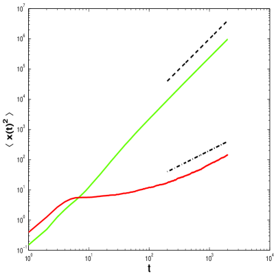
Figure 3: Second moments of the particle position versus time for the velocity field (44). The graphs of $t$ and $t^{2}$ are also included for comparison.

and hence we expect diffusive long time behavior along the $z_{1}$ direction and ballistic motion along the $z_{2}$ direction. In Figure 3 we present the second moments $\langle x_{1}(t)^{2}\rangle,\,\langle x_{2}(t)^{2}\rangle$ of solutions to equation (1) with $v(x)$ given by (44).

4.6 Homogenization When the Centering Hypothesis (32) is not Satisfied

In the previous section we imposed the centering condition (32) in order to ensure that there is no mean drift and that the motion of the inertial particles at long scales is diffusive. In the case where this condition is not satisfied, then we expect that the effective behavior of the particles is described by a transport equation and that the diffusion appears only as a higher order correction. Indeed, an analysis similar to the one presented in the previous section, using the advective rescaling $t=t/\epsilon$ and $x=x/\epsilon,$ shows that in this case the particle motion at large scales is goverened by the following backward Kolmogorov equation

$$\frac{\partial u}{\partial t}=\langle v_{i}\rangle_{\rho}\frac{\partial u}{\partial x_{i}}+\epsilon{\mathcal{K}}_{ij}\frac{\partial^{2}u}{\partial{x_{i}}\partial{x_{j}}},$$

where $\langle v\rangle_{\rho}=\int_{{\mathbb{T}}^{d}}\int_{{\mathbb{R}}^{d}}v(z)\rho(y,z)\,dydz$. Alternatively, the behavior of the particles is diffusive at the reference frame moving with the mean flow.

4.7 The Homogenization Problem for Equation (4)

Let us now consider the equation (4) in the presence of molecular diffusion. For steady flows this equation becomes

$$\ddot{x}=\delta v(x)\cdot\nabla v(x)+\frac{1}{\tau}\left(v(x)-\dot{x}+\sigma\dot{\beta}\right),$$ (45)

where $\delta$ is the ratio of fluid density to particle density. The techniques developed in [25] enable us to conclude that there exists a unique, smooth, invariant density for the process $\{x(t),\,\sqrt{\tau}\dot{x}(t)\}$, which we denote by $\rho^{\delta}(y,z)$. It is straightforward to check that the assumption $v(-z)=-v(z)$ ensures that the drift term $b^{\delta}(z)=\delta v(z)\cdot\nabla v(z)+\frac{1}{\tau}v(z)$ is centered with respect to this invariant density, $\langle b^{\delta}\rangle_{\rho^{\delta}}=0$. Hence, the multiscale techniques developed in section 3 apply with $\frac{1}{\tau}v(z)\to b^{\delta}(z)$ and we can conclude that the rescaled process $x^{\epsilon}=\epsilon x(t/\epsilon^{2})$, with $x(t)$ being the solution of equation (45), converges as $\epsilon\rightarrow 0$ to a Brownian motion. The covariance–effective diffusivity– of this Brownian motion is

$${\mathcal{K}}^{\delta}=\frac{1}{\sqrt{\tau}}\langle\Phi^{\delta}\otimes y\rangle_{\rho^{\delta}}$$

where $\Phi^{\delta}$ solves the cell problem

$${\mathcal{L}}^{\delta}\Phi^{\delta}=-\frac{1}{\sqrt{\tau}}y,$$ (46)

with

$${\mathcal{L}}^{\delta}=\left(\sqrt{\tau}b^{\delta}\cdot\nabla_{y}+\frac{1}{\sqrt{\tau}}y\cdot\nabla_{x}\right)+\frac{1}{\tau}{\mathcal{L}}_{OU}.$$

Now the effective diffusivity depends on $\delta$ as well as on $\tau$ and $\sigma.$ We study the effect of varying $\delta$ in section 6, by means of numerical experiments. The main interest here stems from the fact that, for $\sigma=0$, equation (4) exhibits effective diffusive behaviour for certain cellular flows and choices of $\delta.$ How this diffusive mechanism interacts with molecular diffusion is a matter of some interest.

5 Small $\tau$ Asymptotics

In this section we show that the effective diffusivity tensor ${\mathcal{K}}={\mathcal{K}}(\tau)$ reduces to the effective diffusivity tensor from first order dynamics, as $\tau\to 0$. To this end we define

$$\mathcal{A}_{0}=\mathcal{L}^{OU},\quad\mathcal{A}_{1}=y\cdot\nabla_{z}+v(z)\cdot\nabla_{y}$$

and then, by polarization, the effective diffusion tensor ${\mathcal{K}}(\tau)$ is determined by (41) with $\chi$ solving (40), $\rho$ solving (30) and

$$\mathcal{L}_{0}=\frac{1}{\tau}\mathcal{A}_{0}+\frac{1}{\sqrt{\tau}}\mathcal{A}_{1}.$$

We wish to expand $\chi$ and $\rho$ in powers of $\tau$ and show that the leading order behaviour of ${\mathcal{K}}(\tau)$ is given by (24). Higher order terms in the small $\tau$ expansion of the effective diffusivity ${\mathcal{K}}(\tau)$ will be computed only for the case of a one dimensional potential flow in section 5.4. Perturbation calculations similar to the ones presented in this section were reported in [43, 44] for linear shear flows.

5.1 Expansion for $\chi$

We set

$$\chi=\chi_{0}+\sqrt{\tau}\chi_{1}+\tau\chi_{2}+\cdots$$

in (40) and then find

$$\mathcal{A}_{0}\chi_{0} =0$$ (47)

$$\mathcal{A}_{0}\chi_{1} =-\mathcal{A}_{1}\chi_{0}$$ (48)

$$\mathcal{A}_{0}\chi_{2} =-a\cdot v-\mathcal{A}_{1}\chi_{1}.$$ (49)

The first of these equations implies that $\chi_{0}=\chi_{0}(z)$ only and the second is soluble because

$$\langle\mathcal{A}_{1}\chi_{0}\rangle_{\rho^{OU}}=\langle y\cdot\nabla_{z}\chi_{0}(z)\rangle_{\rho^{OU}}=0.$$

Here $\rho^{OU}$ is the mean zero Gaussian invariant density of the OD process, satisfying (29). Solving for $\chi_{1}$ gives

$$\chi_{1}=y\cdot\nabla_{z}\chi_{0}(z)+\psi_{1}(z)$$

and the solvability condition for the $\chi_{2}$ equation yields

$$\frac{\sigma^{2}}{2}\Delta_{z}\chi_{0}+v(z)\cdot\nabla_{z}\chi_{0}=-a.v(z).$$

Thus $\chi_{0}$ is the solution of the cell problem arising in the passive tracer case, equation (18). Furthermore $\nabla_{y}\chi_{1}=\nabla_{z}\chi_{0}(z)$ and hence

$$\nabla_{y}\chi=\sqrt{\tau}\nabla_{z}\chi_{0}(z)+{\cal O}(\tau).$$ (50)

Notice that the function $\psi_{1}(z)$ is undetermined at this point, but that it does not enter equation (50).

5.2 Expansion For $\rho$

Now it remains to expand $\rho(y,z)$ from (30) in $\tau.$ Notice that

$$\mathcal{A}_{0}^{*}\rho^{OU}(y)=0,\quad\nabla_{y}\rho^{OU}(y)=-2y\rho^{OU}(y)/\sigma^{2}.$$

Then, by (16) with $z\to y$ and $\mathcal{L}_{0}\to\mathcal{A}_{0}$ we find that

$$\mathcal{A}_{0}^{*}(f\rho^{OU}) =-\rho^{OU}[\mathcal{A}_{0}f-\sigma^{2}\Delta_{y}f+2y\cdot\nabla_{y}f]$$

$$=\rho^{OU}\mathcal{A}_{0}f.$$

Let $\rho=\rho^{OU}\hat{\pi}.$ Then

$$0 =\mathcal{L}_{0}^{*}(\rho^{OU}\hat{\pi})$$

$$=\frac{1}{\tau}\mathcal{A}_{0}^{*}(\rho^{OU}\hat{\pi})+\frac{1}{\sqrt{\tau}}\mathcal{A}_{1}^{*}(\rho^{OU}\hat{\pi})$$

$$=\frac{\rho^{OU}}{\tau}\mathcal{A}_{0}\hat{\pi}+\frac{\rho^{OU}}{\sqrt{\tau}}\left(y\cdot\nabla_{z}\hat{\pi}+v\cdot\nabla_{y}\hat{\pi}-\frac{2}{\sigma^{2}}(v\cdot y)\hat{\pi}\right).$$

Since $\rho^{OU}>0$ everywhere we may divide through by it in the above expression. If we then set

$$\hat{\pi}=\pi_{0}+\sqrt{\tau}\pi_{1}+\tau\pi_{2}$$

we find that

$$-\mathcal{A}_{0}\pi_{0} =0$$

$$-\mathcal{A}_{0}\pi_{1} =y\cdot\nabla_{z}\pi_{0}+v\cdot\nabla_{y}\pi_{0}-\frac{2}{\sigma^{2}}(v\cdot y)\pi_{0}$$

$$-\mathcal{A}_{0}\pi_{2} =y\cdot\nabla_{z}\pi_{1}+v\cdot\nabla_{y}\pi_{1}-\frac{2}{\sigma^{2}}(v\cdot y)\pi_{1}.$$

The first equation shows that $\pi_{0}=\pi_{0}(z)$ only and the second then gives

$$\pi_{1}(y,z)=y\cdot\{\nabla_{z}\pi_{0}-\frac{2}{\sigma^{2}}\pi_{0}v\}-\mu_{1}.$$

As with the second term in the dual expansion, the function $\mu_{1}$ is undetermined at this point. However, as the subsequent calculations will show, it is not needed in order to compute the first term in the small $\tau$ expansion of the effective diffusivity.

The negative of the right hand side of the third equation is

$$-y\otimes y:\{D_{z}^{2}\pi_{0}-\frac{2}{\sigma^{2}}\nabla_{z}\{\pi_{0}v\}\}-v\cdot\{\nabla_{z}\pi_{0}-\frac{2}{\sigma^{2}}\pi_{0}v\}$$

$$+y\otimes y:\{\nabla_{z}\pi_{0}-\frac{2}{\sigma^{2}}\pi_{0}v\}\otimes\frac{2v}{\sigma^{2}}+y\cdot\{\nabla_{z}\mu_{1}-\frac{2}{\sigma^{2}}v\mu_{1}\}.$$

Now

$$\langle y\otimes y\rangle_{\rho^{OU}}=\frac{\sigma^{2}}{2}I\quad\mbox{and}\quad\langle y\rangle_{\rho^{OU}}=0$$

and so the solvability condition for $\pi_{2}$ yields

$$-\frac{\sigma^{2}}{2}\Delta_{z}\pi_{0}+\nabla_{z}\cdot\{\pi_{0}v\}=0$$

and hence shows that $\pi_{0}$ coincides with the passive tracer case, equation (11). In summary, we have shown that

$$\rho(y,z)=\rho^{OU}(y)\pi_{0}(z)+{\cal O}(\sqrt{\tau})$$ (51)

where $\pi_{0}(z)$ is the invariant density from the first order dynamics, satisfying (11).

5.3 Limit of the Diffusivity Tensor

Combining (50) and (51) in (41) gives

$$a\cdot{\mathcal{K}}a=\frac{\sigma^{2}}{2}|a|^{2}+\frac{\sigma^{2}}{2}\int_{\mathbb{T}^{d}}\pi(z)|\nabla_{z}\chi_{0}(z)|^{2}dz+\sigma^{2}\int_{\mathbb{T}^{d}}\pi(z)a.\nabla_{z}\chi_{0}(z)+{\cal O}(\sqrt{\tau})$$

which, to leading order in $\tau$, is the expression for the first order dynamics.

5.4 One dimensional Potential Flows

The calculation of higher order terms in the small $\tau$ expansion for the effective diffusivity is quite involved. Moreover, in the general case, these higher order terms do not seem to be of definite sign. However, it is possible to compute explicitly the next term in the small $\tau$ expansion and to prove that it has a definite sign in the case of one dimensional potential flows and we now pursue this. Consider the equation

$$\tau\ddot{z}=-V^{\prime}(z)-\dot{z}+\sigma\dot{\beta}.$$ (52)

In this case we only need to solve perturbatively the cell problem (35) since the stationary Fokker–Planck equation corresponding to (52) is exactly solvable yielding an invariant density independent of $\tau$:

$$\rho(y,z)=\frac{1}{Z}\frac{1}{\sqrt{\pi\sigma^{2}}}e^{-\frac{2}{\sigma^{2}}\left(\frac{1}{2}y^{2}+V(z)\right)},$$ (53)

with $Z=\int_{0}^{1}\exp(-\frac{2}{\sigma^{2}}V(z))\,dz$ and $y=\frac{1}{\sqrt{\tau}}\dot{z}$. The effective diffusivity–which now is a scalar– is given by the formula:

$$\mathcal{K}=\frac{1}{\sqrt{\tau}}\int_{-\infty}^{+\infty}\int_{0}^{1}y\phi(y,z)\rho(y,z)\,dydz.$$ (54)

A lengthy calculation enables us to compute the first four terms in the small $\tau$ expansion for the cell problem:

$$\phi_{0}=\chi(z),$$ (55a)

$$\phi_{1}(y,z)=y(\chi^{\prime}(z)+1),$$ (55b)

$$\phi_{2}(y,z)=\frac{1}{2}y^{2}\chi^{\prime\prime}(z)+\psi_{2}(z),$$ (55c)

$$\phi_{3}(y,z)=\frac{1}{6}y^{3}\chi^{\prime\prime\prime}(z)+y\left(\frac{1}{2}\sigma^{2}\chi^{\prime\prime\prime}(z)-V^{\prime}(z)\chi^{\prime\prime}(z)+\psi_{2}^{\prime}(z)\right).$$ (55d)

The cell problem for the first order dynamics, equation (13), can be solved explicitly [46] to give

$$\chi(z)=\int_{0}^{z}\widehat{\rho}(z)\,dz-z+c_{0},$$

with

$$\widehat{\rho}(z)=e^{\frac{2}{\sigma^{2}}V(z)},\quad\widehat{Z}=\int_{0}^{1}e^{\frac{2}{\sigma^{2}}V(z)}\,dz.$$

We use the above formula for $\chi(z)$ in equation (15) to obtain the following formula for the effective diffusivity

$$\mathcal{K}(\tau=0)=\frac{\sigma^{2}}{2}\frac{1}{Z\widehat{Z}}.$$ (56)

The term $\psi_{2}(z)$ satisfies an equation similar to the cell problem of the first order dynamics. The solution of this equation is

$$\psi_{2}(z)=-\frac{2}{\sigma^{2}}\int_{0}^{z}\left(\frac{1}{2}(V^{\prime}(z))^{2}+\frac{3\sigma^{2}}{4}V^{\prime\prime}(z)\right)\widehat{\rho}(z)\,dz+c_{1}\int_{0}^{z}\widehat{\rho}(z)\,dz+c_{2},$$

where

$$c_{1}=-\frac{2}{\sigma^{2}}\int_{0}^{z}\frac{1}{2}(V^{\prime}(z))^{2}\widehat{\rho}(z)\,dz.$$

The values of the constants $c_{0},\,c_{2}$ are not needed for the computation of the effective diffusivity. We substitute now (55d) and (53), using the formulas for $\chi(z)$ and $\psi_{2}(z)$ and for the moments of the Ornstein–Uhlenbeck process. The final result is

$$\mathcal{K}=\frac{\sigma^{2}}{2}\frac{1}{Z\widehat{Z}}-\tau\int_{0}^{1}\frac{1}{2}(V^{\prime}(z))^{2}\widehat{\rho}(z)\,dz+{\mathcal{O}}(\tau^{2}).$$

The above formula shows that, for $\tau$ sufficiently small, the diffusivity is depleted beyond the depletion exhibited by homogenization in the passive tracer case, which is given by (56).

6 Numerical Experiments

In this section we study the dependence of the effective diffusivity for equations (1), (3) on the non–dimensional parameters of the problem $\tau,\,\sigma$ and $\delta$. For simplicity all the experiments we perform are for the Taylor–Green flow (2)

$$U(x)=\nabla^{\bot}\psi_{TG}(x),\quad\psi_{TG}(x)=\sin(x_{1})\sin(x_{2}).$$

The closed streamlines of Lagrangian particle paths in this velocity field is a rather special situation and we describe numerical experiments for other stream functions, including open streamline topologies, in [34].

It is straightforward to check that the Taylor–Green flow satisfies condition (43) and hence the absence of ballistic motion at long scales is ensured. Moreover, the symmetry properties of (2) imply that the two diagonal components of the effective diffusivity are equal, whereas the off–diagonal components vanish. In the figures presented below we use the notation $K:={\mathcal{K}}_{11}={\mathcal{K}}_{22}$.

Rather than solving the cell problem (46), we compute the effective diffusivity using Monte Carlo simulations: we solve the equations of motion (45) numerically for different realizations of the noise and we compute the effective diffusivity through the formula

$$\mathcal{K}=\lim_{t\rightarrow\infty}\frac{1}{2t}\langle(x(t)-\langle x(t)\rangle)\otimes(x(t)-\langle x(t)\rangle)\rangle,$$

where $\langle\cdot\rangle$ denotes ensemble average. We solve the stochastic equations of motion using Milstein’s method, appropriately modified for the second order SDE [19, p. 386]:

$$x_{n+2}=(2-r)x_{n+1}-(1-r)x_{n}+r\Delta tv(x_{n+1})+\sigma r\Delta t\mathcal{N}(0,1).$$

where $r=\frac{\Delta t}{\tau}$ and $s_{1}=1-\frac{r}{2},\;\;s_{2}=1+\frac{r}{2}.$. This method has strong order of convergence $1.0$. We use $N=1024$ uniformly distributed particles in $2\pi\mathbb{T}^{2}$ with zero initial velocities and we integrate over a very long time interval (which is chosen to depend upon the parameters of the problem) with $\Delta t\approx 5.10^{-4}\min\{1,\tau\}$.

In some instances we compare the effective diffusivities for inertial particles with those for passive tracers. The latter are computed by solving the cell problem directly, by means of a spectral method similar to that described in [24], together with extrapolation into parameter regimes where the dependence of the diffusivity is provably linear.

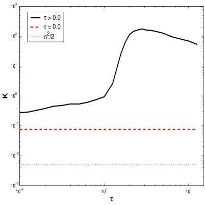
Figure 4: Effective diffusivity versus $\tau$ for $\delta=0.0,\sigma=0.1$ .

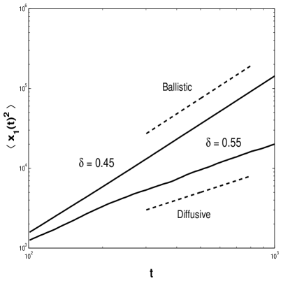
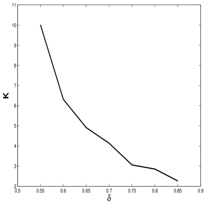
a.   The second moment of the particle velocity for $\delta=0.45$ and $\delta=0.55$. The lines $t$ and $t^{2}$ are also plotted for comparison. b.   ${\mathcal{K}}$ vs $\delta$

Figure 5: Effective diffusivity as a function of $\delta$ for $\sigma=0.0$ and $\tau=2.0$.

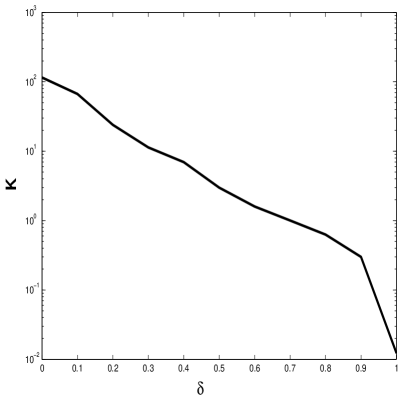
Figure 6: Effective diffusivity as a function of $\delta$ for $\sigma=0.1$ and $\tau=2.0$.

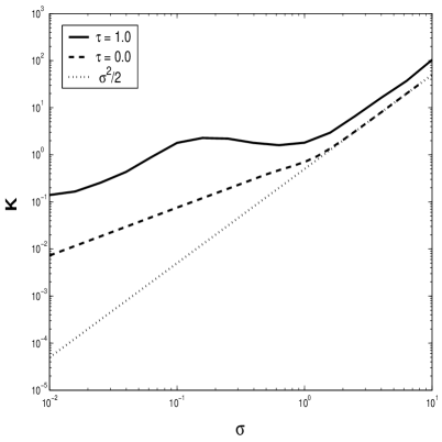
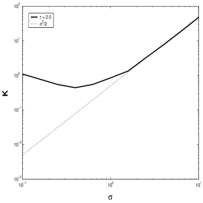
a.   $\delta=0.0,\,\tau=1.0$ b.   $\delta=0.7,\,\tau=2.0$

Figure 7: Effective Diffusivity versus $\sigma$ for $\delta=0.0$ and $\delta=0.7$ .

6.1 The Effect of $\tau$ on Diffusivity

We compute the effective diffusivity as a function of the non–dimensional particle relaxation time $\tau$ for the Taylor–Green flow when $\delta=0.0$. Our results are presented in Figure 4, for $\sigma=0.1$. For comparison, the effective diffusivity of the tracer particle ($\tau=0$) and that of the free particle, namely $\frac{\sigma^{2}}{2}$, are also plotted. The parameter $\tau$, apart from influencing the effective diffusivity, introduces an additional time scale into the problem [20]. In particular, for $\tau$ large, we need to integrate the equations of motion over a longer time interval in order to compute accurate statistics.

The main interest in this data is that it shows highly non–trivial dependence of the effective diffusivity on the parameter $\tau$ as well as giving quantative information about how inertia enhances the diffusivity over that obtained in the case of passive tracers. We remark, in particular, that the effective diffusivity reaches its maximum for $\tau={\mathcal{O}}(1)$. It is in this regime that the free-flight time-scale for the inertial particle is of the same order as that induced by the velocity field. A similar phenomenon, in a different context, has been observed by Vassilicos et. al. [45].

6.2 The Effect of $\delta$ on Diffusivity

It is a well documented result [6, 37, 47, 48, 26] that the particle trajectories of (4) perform an effective Brownian motion even in the absence of noise, in certain parameter regimes. The linear stability analysis of (4) for the Taylor–Green flow indicates that in the parameter regime $\delta\in(1/\tau,1)$ we expect a very complicated, chaotic behavior which might be interpreted as an effective Brownian motion at long times. When $U(x)=\nabla^{\bot}\psi_{TG}(x)$ then the noise free dynamics arising from (1) when $\sigma=0$ has two sets of equilibria, $X_{0}^{1}=[n\pi,0,m\pi,0],\,n,m\in\mathbb{N}$ and $X_{0}^{2}=[\frac{\pi}{2}+n\pi,0,\frac{\pi}{2}+m\pi,0],\,n,m\in\mathbb{N}$. The first set of equilibria have two dimensional unstable manifold for $\delta>\tau^{-1}$ and one dimensional for $\delta<\tau^{-1}$; the second set have a two dimensional unstable manifold for $\delta<1$ and is stable for $\delta>1.$ Numerically we observe diffusive behaviour, in the absence of noise, if and only if $\delta\in(\tau^{-1},1).$ In this regime, all equilibria have two dimensional unstable manifolds. The basic mechanism for diffusion is chaotic mixing caused by separation near the separatrices of equilibria; it is unsurprising therefore that the linear stability of equilibria play a strong role on determining the interval of $\delta$ in which diffusion occurs.

In Figure 5a we plot the second moment of the particle position as a function of time for values of $\delta$ below and above the threshold $\delta=0.5$, and in the absence of noise. As expected, the particle motion is ballistic for $\delta=0.45$ and diffusive for $\delta=0.55$.

In Figure 5b we plot the effective diffusivity as a function of $\delta$, again in the absence of noise. Since we have chosen $\tau=2.0$ we expect an effective Brownian motion for $\delta\in(0.5,1)$. Notice that the effective diffusivity increases as $\delta\rightarrow 0.5^{+}$, and appears to diverge in the limit. This is to be expected, since $\delta=0.5$ separates ballistic motion (for $\delta<0.5$) and diffusive motion (for $\delta>0.5$) motion.

In Figure 6 we plot the effective diffusivity as a function of $\delta$ when the particles are subject to additional molecular diffusion. In this case the effective diffusivity is a decreasing function of $\delta$.

6.3 The Effect of $\sigma$ on Diffusivity

It is well known, see e.g. [23], that for the case of passive tracers the effective diffusivity depends on the molecular diffusivity $\sigma$ in a highly non–linear, very complicated way. In particular, the limit as $\sigma$ tends to $0$ is singular and the enhancement in the diffusivity–for divergence free flows– depends crucially on the topology of the streamlines. It is therefore interesting to study the dependence of the effective diffusivity on $\sigma$ for the inertial particles problem.

In Figure 7 we present the effective diffusivity as a function of the molecular diffusion for two sets of parameters: (a) for $\delta=0.0$ (for which the streamlines are closed), $\tau=1.0$ and (b) for $\delta=0.7,\,\tau=2.0$ (a regime in which there exists a well defined effective diffusivity even in the respectively. The diffusivity of the free particle $\frac{\sigma^{2}}{2}$ is also plotted for comparison. Moreover, in Figure 7(a), we also plot the effective diffusivity for passive tracers.

In both figures we see the clear enhancement of diffusivity over the bare molecular value. Furthermore, in Figure 7(a) we also observe that the enhancement in the diffusivity is significantly greater for $\tau>0$ (inertial particles) than it is for $\tau=0$ (passive tracers), especially when $\sigma$ is small.

A further interesting observation concerns the dependence of the diffusivity on $\sigma$. For $\delta=0$ the dependence is highly non-trivial, exhibiting both a local maximum and a local minimum. For $\delta=0.7$ the presence of inertia leads to an effective diffusivity which increases as $\sigma$ becomes smaller. This should be contrasted with the established fact that, for passive tracers in periodic cellular flows, the effective diffusivity decreases linearly in $\sigma$, for $\sigma$ sufficiently small [39, 42]. It would be interesting to understand how the enhancement scales with $\sigma\rightarrow 0$ and to compare it with known theoretical results for the passive tracer case; in particular, it would be interesting to extend the theory of maximally and minimally enhanced diffusion [24] to the inertial situation studied here.

7 Conclusions

The problem of periodic homogenization for inertial particles is considered in this paper. It is shown that, at long times and large scales, the inertial particles perform Brownian motion and a formula for the effective diffusivity is derived. Furthermore, the dependence of the effective diffusivity on the non–dimensional particle mass $\tau$ a(Stokes number) and the ratio of the fluid to particle density $\delta$ is studied, by means of analysis and numerics.

It is shown that, as $\tau\rightarrow 0,$ the effective diffusivity converges to the one obtained from the homogenization of passive tracers. Moreover, it is shown through numerical experiments that for a variety of interesting divergence free flows, the diffusivity in the presence of inertia is enhanced much beyond the well documented enhancement of the diffusivity for passive tracers. Furthermore, the dependence of the effective diffusivity on $\tau$ and $\delta$ is studied numerically in some detail.

The calculation of the effective diffusion tensor requires the numerical solution of equations (35) and (30). It is coneivable that this task might be as computationally demanding as direct Monte Carlo simulations, because the domain of the PDE is unbounded in the momentum variable, and because the PDE is not elliptic (only hypo-elliptic). This is to be contrasted to the case of passive tracers in periodic flows; there the calculation of the effective diffusivity requires the solution of the elliptic PDE (13) on a periodic domain. Equations of this type can be routinely and effeciently solved using, for example, a spectral method. From this point of view our results might not provide any computational advantage over Monte Carlo simulations. However, the results reported in this paper provide a mathematical framework for rigorous analysis of the dependence of the effective diffusion coefficient on the physical parameters of the problem. We have already undertaken such an analysis to study the limit of small Stokes number and we plan to undertake further studies in future work.

The numerical results reported in section 6, for a simple two– dimensional steady flow, exhibit a wide range of interesting physical phenomena. As examples we mention the dependence of the effective diffusivity on the Stokes number and the fluid/particle density ratio, for a given streamline topology, question which are, we believe, of great interest to the applied community. The purpose of this work is to develop a framework within which such questions can be addressed. We plan to investigate some of these issues in future work. The dependence of the effective diffusivity for a wider class of velocity fields is undertaken in [34].

Summarizing, we note the following specific areas where future work would be of interest:

• the extension to time dependent velocity fields $v(x,t)$, either periodic in time or random in time – for example with an Ornstein–Uhlenbeck structure as in [33, 40, 41];

• the extension to random velocity fields in space;

• rigorous analysis of the parametric dependence of the effective diffusivity on $\sigma$, $\tau$ and $\delta$, taking into account the free streamline topologies;

• further numerical studies for velocity fields other than the simple Taylor Green flows studied here – in particular to study problems where the Lagrangian particle paths have open streamline topologies, such as the Childress-Soward family; this is initiated in [34].

Appendix A Appendix

In this appendix we prove the existence of a unique invariant measure for the process $\{x,\dot{x}\}$ solving (1) and, moreover, that the generator ${\mathcal{L}}$ of the process satisfies the Fredholm alternative. This justifies the formal multi–scale calculations presented in section 3. To simplify the notation we set $\sigma=\tau=1$. The equations of motion become

$$\ddot{x}=v(x)-\dot{x}+\dot{\beta}.$$ (57)

The generator of the Markov process $\{x,y\}$, with $y=\dot{x}$ is

$${\mathcal{L}}=y\cdot\nabla_{x}+\left(v(x)-y\right)\cdot\nabla_{y}+\frac{1}{2}\Delta_{y}$$

We have the following theorem

Theorem A.1.

Assume that $v(x)\in C^{\infty}({\mathbb{T}}^{d})$. Then there exists a unique, smooth invariant density $\rho(x,y)$ for the process $\{x,y\}$:

$${\mathcal{L}}^{*}\rho(x,y)=0.$$

Let further $h(x,y)$ be a smooth function such that $\int_{{\mathbb{R}}^{d}}\int_{T^{d}}h(x,y)\rho(x,y)\,dxdy=0$. Then the Poisson equation

$$-{\mathcal{L}}f=h$$ (58)

has a unique mean zero solution in $L^{2}({\mathbb{T}}^{d}\times{\mathbb{R}}^{d},e^{-\delta^{2}\|y\|^{2}}dxdy)$ for every $\delta\in(0,2\sigma^{-2})$.

The proof of the existence of a unique invariant measure for our process is based on the results of [25] and is broken into three lemmas. First, we need to prove the existence of a smooth transition probability density for our Markov process. This is accomplished by means of Hörmander’s theorem [36, Thm V38.16]. Then we need to prove the compactness of phase space, for which we need to find an appropriate Lyapunov functions. Finally, we need to prove that the transition probability density is everywhere positive. To show this we need to use a controllability argument. The proof of the existence and uniqueness of solutions of the Poisson equation (58) is based on Fredholm’s theorem.

Lemma A.1.

The Markov process generated by ${\mathcal{L}}$ has a smooth transition probability density.

Proof.

This follows by an application of Hörmander’s theorem. The basic idea behind this theorem is that, even though noise does not act directly to the position variable, there is nevertheless sufficient interaction between momentum and position so that noise, and consequently smoothness, is transmitted to all degrees of freedom. We write the generator in Hörmander’s ”sum of squares” form:

$${\mathcal{L}}=\frac{1}{2}\sum_{i=1}^{d}X_{i}^{2}+X_{0},$$

where $X_{i}=\frac{\partial}{\partial y_{i}},\,i=1,\dots d$ and $X_{0}=y\cdot\nabla_{x}+\left(v(x)-y\right)$. Let now $[A,B]$ denote the commutator between the vector fields $A,\,B$ and let $\mbox{Lie}\{F\}$ denote the Lie algebra generated by the family of vector fields $F$. Define

$$\mathcal{A}_{0}=\mbox{Lie}\{X_{1},\dots X_{d}\}$$

and

$$\mathcal{A}_{k}=\mbox{Lie}\{[X_{0},U],\,U\in\mathcal{A}_{k-1}\},\,k=1,2,\dots$$

Set finally

$$\mathcal{H}=\mbox{Lie}\{\mathcal{A}_{0},\mathcal{A}_{1}\dots\}.$$

According to Hörmander’s theorem, a sufficient condition for the Markov process $\{x,y\}$ to possess a smooth invariant density is for $\mathcal{H}$ to span the tangent space $T_{x,y}M$, where $M={\mathbb{T}}^{d}\times{\mathbb{R}}^{d}$. We readily check now that

$$[X_{0},X_{i}]=-\frac{\partial}{\partial x_{i}}+\frac{\partial}{\partial y_{i}},\quad i=1,\dots d,$$

and consequently

$$\mbox{Span}\left(\mbox{Lie}\left\{\mathcal{A}_{0},\mathcal{A}_{1}\right\}\right)=T_{x,y}M.$$

Thus, Hörmander’s hypothesis is satisfied and the Markov process generated by ${\mathcal{L}}$ has a smooth density. ∎

Now we prove that the existence of a Lyapunov function.

Lemma A.2.

There exists a constant $\beta>0$ such that the function $V(x,y)=1+\frac{1}{2}\|y\|^{2}$ satisfies

$${\mathcal{L}}(V(x,y))\leq-\frac{1}{2}V(x,y)+\beta.$$

Proof.

We have that $V(x,y)$ maps the state space onto $[1,\infty)$ and that $\lim_{\|y\|\rightarrow\infty}V(x,y)=\infty$. Moreover we have

$${\mathcal{L}}(V(x,y)) = v\cdot y-\|y\|^{2}+\frac{d}{2}$$ (59)

$$\leq -\frac{1}{2}\|y\|^{2}+\left(\frac{d}{2}+\frac{1}{2}\|v\|^{2}\right)$$

$$\leq -V(x,y)+\beta,$$

with $\beta=d/2+(1/2)\sup_{x\in{\mathbb{T}}^{d}}\|v(x)\|^{2}+1$. ∎

The last ingredient which is needed for the proof of the ergodicity of the process generated by ${\mathcal{L}}$ is the fact the transition probability $P_{t}$ is everywhere positive.

Lemma A.3.

For all $z:=(x,y)\in{\mathbb{T}}^{d}\times{\mathbb{R}}^{d},t>0$ and open $\mathcal{O}\subset{\mathbb{T}}^{d}\times{\mathbb{R}}^{d}$, the transition kernel for (57) satisfies $P_{t}(z,\mathcal{O})>0$.

For the proof of this lemma we refer to [25, Lemma 3.4].

Proof of Theorem A.1. The existence of a unique invariant measure follows from Lemmas A.1, A.2 and A.3, upon using Corollary 2.8 from [25]. In order to prove the existence and uniqueness of solutions of the Poisson equation (58) we need to prove that the generator ${\mathcal{L}}$ has compact resolvent. This is accomplished in [16, Thm 3.1, Thm 3.2]. ∎

Remark A.1.

The above lemmas enable us to conclude that the system converges exponentially fast to its invariant distribution [25].

Remark A.2.

We a bit of extra work we can also prove sharp estimates for the invariant distribution and the solution of the Poisson equation $-{\mathcal{L}}f=h$. We refer to [16, Thm 3.1, Thm 3.2] for details.

References

- [1] G. Allaire. Homogenization and two-scale convergence. SIAM J. Math. Anal., 23(6):1482–1518, 1992.
- [2] H. Aref, S.W. Jones, S. Mofina, and I. Zawadzki. Vortices, Kinematics and chaos. Phys. D, 37(1-3):423–440, 1989.
- [3] R. Battacharya. A central limit theorem for diffusions with periodic coefficients. The Annals of Probability, 13:385–396, 1985.
- [4] A. Bensoussan, J.L. Lions, and G. Papanicolaou. Asymptotic analysis of periodic structures. North-Holland, Amsterdam, 1978.
- [5] P. Castiglione and A. Crisanti. Dispersion of passive tracers in a velocity field with non-- corellated noise. Phys. Rev. E, 59(4):3926–3934, 1999.
- [6] A. Crisanti, M. Falcioni, A. Provenzale, and A. Vulpiani. Passive advection of particles denser than the surrounding fluid. Phys. Let. A, 150(2):79–84, 1990.
- [7] G. T. Csanady. Turbulent Diffusion in the Enviroment. D. Reidel, Dordrecht, 1973.
- [8] J.K. Eaton and J.R. Fessler. Preferential concetration of particles by turbulence. Int. J. Mult. Flow, 20:169–209, 1994.
- [9] S.N. Ethier and T.G. Kurtz. Markov processes. Wiley Series in Probability and Mathematical Statistics: Probability and Mathematical Statistics. John Wiley & Sons Inc., New York, 1986.
- [10] G. Falkovich, A. Fouxon, and M.G. Stepanov. Acceleration of rain initiation by cloud turbulence. Nature, 419:151–154, 2002.
- [11] G. Falkovich, K. Gawȩdzki, and M. Vergassola. Particles and fields in fluid turbulence. Rev. Modern Phys., 73(4):913–975, 2001.
- [12] A. Fannjiang and G.C. Papanicolaou. Convection enhanced diffusion for periodic flows. SIAM J. APPL. MATH, 54:333–408, 1994.
- [13] M. Freidlin. Some remarks on the Smoluchowski–Kramers approximation. J. Statist. Phys., to appear, 2004.
- [14] C. W. Gardiner. Handbook of stochastic methods. Springer-Verlag, Berlin, second edition, 1985. For physics, chemistry and the natural sciences.
- [15] J. Garnier. Homogenization in a periodic and time-dependent potential. SIAM J. APPL. MATH, 57(1):95–111, 1997.
- [16] M. Hairer and G. A. Pavliotis. Periodic homogenization for hypoelliptic diffusions. J. Stat. Phys., 117(1/2):261–279, 2004.
- [17] I. Karatzas and S.E. Shreve. Brownian Motion and Stochastic Calculus, volume 113 of Graduate Texts in Mathematics. Springer-Verlag, New York, second edition, 1991.
- [18] C. Kipnis and S. R. S. Varadhan. Central limit theorem for additive functionals of reversible Markov processes and applications to simple exclusions. Comm. Math. Phys., 104(1):1–19, 1986.
- [19] P.E. Kloeden and E. Platen. Numerical solution of stochastic differential equations, volume 23 of Applications of Mathematics (New York). Springer-Verlag, Berlin, 1992.
- [20] A.M. Lacasta, J.M Sancho, A.H. Romero, I.M. Sokolov, and K. Lindenberg. From subdiffusion to superdiffusion of particles on solid surfaces. Phys. Rev. E, 70:051104, 2004.
- [21] A. Lasota and M.C. Mackey. Chaos, Fractals, Noise. Springer-Verlag, New York, 1994.
- [22] J.L. Lebowitz and H. Rost. The Einstein relation for the displacement of a test particle in a random environment. Stochastic Process. Appl., 54(2):183–196, 1994.
- [23] A.J. Majda and P.R. Kramer. Simplified models for turbulent diffusion: Theory, numerical modelling and physical phenomena. Physics Reports, 314:237–574, 1999.
- [24] A.J. Majda and R.M. McLaughlin. The effect of mean flows on enhanced diffusivity in transport by incompressible periodic velocity fields. Studies in Applied Mathematics, 89:245–279, 1993.
- [25] J.C. Mattingly and A. M. Stuart. Geometric ergodicity of some hypo-elliptic diffusions for particle motions. Markov Processes and Related Fields, 8(2):199–214, 2002.
- [26] M.R. Maxey. The motion of small spherical particles in a cellular flow field. Phys. Fluids, 30(7):1915–1928, 1987.
- [27] M.R. Maxey. On the advection of spherical and nonspherical particles in a nonuniform flow. Philos. Trans. Roy. Soc. London Ser. A, 333(1631):289–307, 1990.
- [28] M.R. Maxey and J.J. Riley. Equation of motion for a small rigid sphere in a nonuniform flow. Phys. Fluids, 26:883–889, 1983.
- [29] D.W. McLaughlin, G.C. Papanicolaou, and O.R. Pironneau. Convection of microstructure and related problems. SIAM J. APPL. MATH, 45:780–797, 1985.
- [30] S. Olla. Homogenization of diffusion processes in random fields. Lecture Notes, 1994.
- [31] G. Papanicolaou and S. R. S. Varadhan. Ornstein-Uhlenbeck process in a random potential. Comm. Pure Appl. Math., 38(6):819–834, 1985.
- [32] E. Pardoux. Homogenization of linear and semilinear second order parabolic pdes with periodic coefficients: A probabilistic approach. Journal of Functional Analysis, 167:498–520, 1999.
- [33] G. A. Pavliotis and A. M. Stuart. White noise limits for inertial particles in a random field. Multiscale Model. Simul., 1(4):527–533 (electronic), 2003.
- [34] G. A. Pavliotis, A.M. Stuart, and L. Band. Monte carlo studies of effective diffusivities for inertial particles. submitted, 2004.
- [35] H. Rodenhausen. Einstein’s relation between diffusion constant and mobility for a diffusion model. J. Statist. Phys., 55(5-6):1065–1088, 1989.
- [36] L. C. G. Rogers and David Williams. Diffusions, Markov processes, and martingales. Vol. 1. Cambridge Mathematical Library. Cambridge University Press, Cambridge, 2000.
- [37] J. Rubin, C. K. R. T. Jones, and M. Maxey. Settling and asymptotic motion of aerosol particles in a cellular flow field. J. Nonlinear Sci., 5(4):337–358, 1995.
- [38] R. A. Shaw. Particle-turbulence interactions in atmosphere clouds. Annu. Rev. Fluid Mech., 35:183–227, 2003.
- [39] B. I. Shraiman. Diffusive transport in a rayleigh-benard convection cell. Phys. Rev. A, 36(1):261–267, 1987.
- [40] H. Sigurgeirsson and A. M. Stuart. Inertial particles in a random field. Stoch. Dyn., 2(2):295–310, 2002.
- [41] H. Sigurgeirsson and A. M. Stuart. A model for preferential concentration. Phys. Fluids, 14(12):4352–4361, 2002.
- [42] T.H. Solomon and J. P. Gollub. Passive transport in steady rayleigh-benard convection. Phys. Fluids, 31(6):1372–1378, 1988.
- [43] G. Subramanian and J. F. Brady. A Chapman-Enskog formalism for inertial suspensions. Phys. A, 334(3-4):385–416, 2004.
- [44] G. Subramanian and J. F. Brady. Multiple scales analysis of the Fokker-Planck equation for simple shear flow. Phys. A, 334(3-4):343–384, 2004.
- [45] J.C. Vassilicos, L. Chen, S. Goto, and D. Osborne. Persistent stagnation points and turbulent clustering of inertial particles. Preprint, 2005.
- [46] M. Vergassola and M. Avellaneda. Scalar transport in compressible flow. Phys. D, 106(1-2):148–166, 1997.
- [47] L.-P. Wang, T.D. Burton, and D.E. Stock. Quantification of chaotic dynamics for heavy particle dispersion in abc flow. Phys. Fluids. A, 3(5):1073–1080, 1991.
- [48] L.P. Wang, M.R. Maxey, T.D. Burton, and D.E. Stock. Chaotic dynamics of particle dispersion in fluids. Phys. Fluids A, 4(8):1789–1804, 1992.