A MULTISCALE APPROACH TO BROWNIAN MOTORS

Abstract

The problem of Brownian motion in a periodic potential, under the influence of external forcing, which is either random or periodic in time, is studied in this paper. Multiscale techniques are used to derive general formulae for the steady state particle current and the effective diffusion tensor. These formulae are then applied to calculate the effective diffusion coefficient for a Brownian particle in a periodic potential driven simultaneously by additive Gaussian white and colored noise. Our theoretical findings are supported by numerical simulations.

1 Introduction

Particle transport in spatially periodic, noisy systems has attracted considerable attention over the last decades, see e.g. [33, Ch. 11], [30] and the references therein. There are various physical systems where Brownian motion in periodic potentials plays a prominent role, such as Josephson junctions [1], surface diffusion [18, 34] and superionic conductors [11]. While the system of a Brownian particle in a periodic potential is kept away from equilibrium by an external, deterministic or random, force, detailed balance does not hold. Consequently, and in the absence of any spatial symmetry, a net particle current will appear, without any violation of the second law of thermodynamics. It was this fundamental observation [21] that led to a revival of interest in the problem of particle transport in periodic potentials with broken spatial symmetry. These types of non– equilibrium systems, which are often called Brownian motors or ratchets, have found new and exciting applications e.g as the basis of theoretical models for various intracellular transport processes such as molecular motors [5]. Furthermore, various experimental methods for particle separation have been suggested which are based on the theory of Brownian motors [4].

The long time behavior of a Brownian particle in a periodic potential is determined uniquely by the effective drift and the effective diffusion tensor which are defined, respectively, as

$$U_{eff}=\lim_{t\rightarrow\infty}\frac{\langle x(t)-x(0)\rangle}{t}$$ (1)

and

$$D_{eff}=\lim_{t\rightarrow\infty}\frac{\langle x(t)-\langle x(t)\rangle)\otimes(x(t)-\langle x(t)\rangle)\rangle}{2t}.$$ (2)

Here $x(t)$ denotes the particle position, $\langle\cdot\rangle$ denotes ensemble average and $\otimes$ stands for the tensor product. Indeed, an argument based on the central limit theorem [3, Ch. 3], [16] implies that at long times the particle performs an effective Brownian motion which is a Gaussian process, and hence the first two moments are sufficient to determine the process uniquely. The main goal of all theoretical investigations of noisy, non–equilibrium particle transport is the calculation of (1) and (2). One wishes, in particular, to analyze the dependence of these two quantities on the various parameters of the problem, such as the friction coefficient, the temperature and the particle mass.

Enormous theoretical effort has been put into the study of Brownian ratchets and, more generally, of Brownian particles in spatially periodic potentials [30]. The vast majority of all these theoretical investigations is concerned with the calculation of the effective drift for one dimensional models. This is not surprising, since the theoretical tools that are currently available are not sufficient for the analytical treatment of the multi–dimensional problem. This is only possible when the potential and/or noise are such that the problem can be reduced to a one dimensional one [9]. For more general multi–dimensional problems one has to resort to numerical simulations. There are various applications, however, where the one dimensional analysis is inadequate. As an example we mention the technique for separation of macromolecules in microfabricated sieves that was proposed in [6]. In the two–dimensional setting considered in this paper, an appropriately chosen driving force in the $y$ direction produces a constant drift in the $x$ direction, but with a zero net velocity in the $y$ direction. On the other hand, a force in the $x$ direction produces no drift in the $y$ direction. The theoretical analysis of this problem requires new technical tools.

Furthermore, the number of theoretical studies related to the calculation of the effective diffusion tensor has also been scarce [12, 20, 31, 32, 35]. In these papers, relatively simple potentials and/or forcing terms are considered, such as tilting periodic potentials or simple periodic in time forcing. It is widely recognized that the calculation of the effective diffusion coefficient is technically more demanding than that of the effective drift. Indeed, as we will show in this paper, it requires the solution of a Poisson equation, in addition to the solution of the stationary Fokker–Planck equation which is sufficient for the calculation of the effective drift. Diffusive, rather than directed, transport can be potentially extremely important in the design of experimental setups for particle selection [30, Sec 5.11] [35]. It is therefore desirable to develop systematic tools for the calculation of the effective diffusion coefficient (or tensor, in the multi–dimensional setting).

From a mathematical point of view, non–equilibrium systems which are subject to unbiased noise can be modelled as non–reversible Markov processes [28] and can be expressed in terms of solutions to stochastic differential equations (SDEs). The SDEs which govern the motion of a Brownian particle in a periodic potential possess inherent length and time scales: those related to the spatial period of the potential and the temporal period (or correlation time) of the external driving force. From this point of view the calculation of the effective drift and the effective diffusion coefficient amounts to studying the behavior of solutions to the underlying SDEs at length and time scales which are much longer than the characteristic scales of the system. A systematic methodology for studying problems of this type, which is based on scale separation, has been developed many years ago [3, 24, 25]. The techniques developed in the aforementioned references are appropriate for the asymptotic analysis of stochastic systems (and Markov processes in particular) which are spatially and/or temporally periodic. The purpose of this work is to apply these multiscale techniques to the study Brownian motors in arbitrary dimensions, with particular emphasis to the calculation of the effective diffusion tensor.

The rest of this paper is organized as follows. In section 2 we introduce the model that we will study. In section 3 we obtain formulae for the effective drift and the effective diffusion tensor in the case where all external forces are Markov processes. In section 4 we study the effective diffusion coefficient for a Brownian particle in a periodic potential driven simultaneously by additive Gaussian white and colored noise. Section 5 is reserved for conclusions. In Appendix A we derive formulae for the effective drift and the effective diffusion coefficient for the case where the Brownian particle is driven away from equilibrium by periodic in time external fluctuations. Finally, in appendix B we use the method developed in this paper to calculate the effective diffusion coefficient of an overdamped particle in a one dimensional tilted periodic potential.

2 The Model

We consider the overdamped $d$–dimensional stochastic dynamics for a state variable $x(t)\in{\mathbb{R}}^{d}$ [30, sec. 3]

$$\gamma\dot{x}(t)=-\nabla V(x(t),f(t))+y(t)+\sqrt{2\gamma k_{B}T}\xi(t),$$ (3)

where $\gamma$ is the friction coefficient, $k_{B}$ the Boltzmann constant and $T$ denotes the temperature. $\xi(t)$ stands for the standard $d$–dimensional white noise process, i.e.

$$\langle\xi_{i}(t)\rangle=0\quad\mbox{and}\quad\langle\xi_{i}(t)\xi_{j}(s)\rangle=\delta_{ij}\delta(t-s),\quad i,j=1,\dots d.$$

We take $f(t)$ and $y(t)$ to be Markov processes with respective state spaces $E_{f},\,E_{y}$ and generators ${\mathcal{L}}_{f},\,{\mathcal{L}}_{y}$. The potential $V(x,f)$ is periodic in $x$ for every $f$, with period $L$ in all spatial directions:

$$V(x+L\hat{e}_{i},f)=V(x,f),\quad i=1,\dots,d,$$

where $\{\hat{e}_{i}\}_{i=1}^{d}$ denotes the standard basis of ${\mathbb{R}}^{d}$. We will use the notation $Q=[0,L]^{d}$.

The processes $f(t)$ and $y(t)$ can be continuous in time diffusion processes which are constructed as solutions of stochastic differential equations, dichotomous noise [15, Ch. 9], more general Markov chains etc. The (easier) case where $f(t)$ and $y(t)$ are deterministic, periodic functions of time is treated in the appendix.

For simplicity, we have assumed that the temperature in (3) is constant. However, this assumption is with no loss of generality, since eqn. (3) with a time dependent temperature can be mapped to an equation with constant temperature and an appropriate effective potential [30, sec. 6]. Thus, the above framework is general enough to encompass most of the models that have been studied in the literature, such as pulsating, tilting, or temperature ratchets. We remark that the state variable $x(t)$ does not necessarily denote the position of a Brownian particle. We will, however, refer to $x(t)$ as the particle position in the sequel.

The process $\{x(t),f(t),y(t)\}$ in the extended phase space ${\mathbb{R}}^{d}\times E_{f}\times E_{y}$ is Markovian with generator

$${\mathcal{L}}=F(x,f,y)\cdot\nabla_{x}+D\Delta_{x}+{\mathcal{L}}_{f}+{\mathcal{L}}_{y},$$

where $D:=\frac{k_{B}T}{\gamma}$ and

$$F(x,f,y)=\frac{1}{\gamma}\left(-\nabla V(x,f)+y\right).$$

To this process we can associate the initial value problem for the backward Kolmogorov Equation [23, Ch. 8]

$$\frac{\partial u}{\partial t}={\mathcal{L}}u,\quad u(x,y,f,t=0)=u_{in}(x,y,f).$$ (4)

which is, of course, the adjoint to the Fokker–Planck equation. Our derivation of formulae for the effective drift and the effective diffusion tensor is based on singular perturbation analysis of the initial value problem (4).

3 Multiscale Analysis

In this section we derive formulae for the effective drift and the effective diffusion tensor for $x(t)$, the solution of (3). Let us outline the basic philosophy behind the derivation of formulae (13) and (18). We are interested in the long time, large scale behavior of $x(t)$. For the analysis that follows it is convenient to introduce a parameter $\epsilon\ll 1$ which in effect is the ratio between the length scale defined through the period of the potential and a large ”macroscopic” length scale at which the motion of the particle is governed by and effective Brownian motion. The limit $\epsilon\rightarrow 0$ corresponds to the limit of infinite scale separation. The behavior of the system in this limit can be analysed using singular perturbation theory.

We remark that the calculation of the effective drift and the effective diffusion tensor are performed seperately, because a different re–scaling is needed in each case. This is due to the fact that advection and diffusion have different characteristic time scales.

3.1 Calculation of the Effective Drift

The backward Kolmogorov equation reads

$$\frac{\partial u(x,y,f,t)}{\partial t}=\left(F(x,f,y)\cdot\nabla_{x}+D\Delta_{x}+{\mathcal{L}}_{f}+{\mathcal{L}}_{y}\right)u(x,y,f,t).$$ (5)

We re–scale a space and time in (5) according to

$$x\rightarrow\epsilon x,\quad t\rightarrow\epsilon t$$

and divide through by $\epsilon$ to obtain

$$\frac{\partial u^{\epsilon}}{\partial t}=\frac{1}{\epsilon}\left(F\left((\frac{x}{\epsilon},f,y\right)\cdot\nabla_{x}+\epsilon D\Delta_{x}+{\mathcal{L}}_{f}+{\mathcal{L}}_{y}\right)u^{\epsilon}.$$ (6)

We solve (6) pertubatively by looking for a solution in the form of a two–scale expansion

$$u^{\epsilon}(x,f,y,t)=u_{0}\left(x,\frac{x}{\epsilon},f,y,t\right)+\epsilon u_{1}\left(x,\frac{x}{\epsilon},f,y,t\right)+\epsilon^{2}u_{2}\left(x,\frac{x}{\epsilon},f,y,t\right)+\dots.$$ (7)

All terms in the expansion (7) are periodic functions of $z=x/\epsilon$. From the chain rule we have

$$\quad\nabla_{x}\rightarrow\nabla_{x}+\frac{1}{\epsilon}\nabla_{z}.$$ (8)

Notice that we do not take the terms in the expansion (8) to depend explicitly on $t/\epsilon$. This is because the coefficients of the backward Kolmogorov equation (6) do not depend explicitly on the fast time $t/\epsilon$. In the case where the fluctuations are periodic, rather than Markovian, in time, we will need to assume that the terms in the multiscale expansion for $u^{\epsilon}(x,t)$ depend explicitly on $t/\epsilon$. The details are presented in the appendix.

We substitute now (7) into (5), use (8) and treat $x$ and $z$ as independent variables. Upon equating the coefficients of equal powers in $\epsilon$ we obtain the following sequence of equations

$${\mathcal{L}}_{0}u_{0} = 0,$$ (9)

$${\mathcal{L}}_{0}u_{1} = -{\mathcal{L}}_{1}u_{0}+\frac{\partial u_{0}}{\partial t},$$ (10)

$$\dots = \dots,$$

where

$$\mathcal{L}_{0}=F(z,f,y)\cdot\nabla_{z}+D\Delta_{z}+{\mathcal{L}}_{y}+{\mathcal{L}}_{f}$$ (11)

and

$${\mathcal{L}}_{1}=F(z,f,y)\cdot\nabla_{x}+2D\nabla_{z}\nabla_{x}.$$

The operator ${\mathcal{L}}_{0}$ is the generator of a Markov process on $Q\times E_{y}\times E_{f}$. In order to proceed we need to assume that this process is ergodic: there exists a unique stationary solution of the Fokker–Planck equation

$${\mathcal{L}}_{0}^{*}\rho(z,y,f)=0,$$ (12)

with

$$\int_{Q\times E_{y}\times E_{f}}\rho(z,y,f)\,dzdydf=1$$

and

$${\mathcal{L}}_{0}^{*}\rho=\nabla_{z}\cdot\left(F(z,f,y)\rho\right)+D\Delta_{z}\rho+{\mathcal{L}}^{*}_{y}\rho+{\mathcal{L}}^{*}_{f}\rho.$$

In the above ${\mathcal{L}}^{*}_{f}$ and ${\mathcal{L}}^{*}_{y}$ are the Fokker–Planck operators of $f$ and $y$, respectively. The stationary density $\rho(z,y,f)$ satisfies periodic boundary conditions in $z$ and appropriate boundary conditions in $f$ and $y$. We emphasize that the ergodicity of the ”fast” process is necessary for the very existence of an effective drift and an effective diffusion coefficient, and it has been tacitly assumed in all theoretical investigations concerning Brownian motors [30].

Under the assumption that (12) has a unique solution eqn. (9) implies, by Fredholm alternative, that $u_{0}$ is independent of the fast scales:

$$u_{0}=u(x,t).$$

Eqn. (10) now becomes

$${\mathcal{L}}_{0}u_{1}=\frac{\partial u(x,t)}{\partial t}-F(z,y,f)\cdot\nabla_{x}u(x,t).$$

In order for this equation to be well posed it is necessary that the right hand side averages to $0$ with respect to the invariant distribution $\rho(z,f,y)$. This leads to the following backward Liouville equation

$$\frac{\partial u(x,t)}{\partial t}=U_{eff}\cdot\nabla_{x}u(x,t),$$

with the effective drift given by

$$U_{eff} = \int_{Q\times E_{y}\times E_{f}}F(z,y,f)\rho(z,y,f)\,dzdydf$$ (13)

$$= \frac{1}{\gamma}\int_{Q\times E_{y}\times E_{f}}\left(-\nabla V(x,f)+y\right)\rho(z,y,f)\,dzdydf.$$

3.2 Calculation of the Effective Diffusion Coefficient

We assume for the moment that the effective drift vanishes, $U_{eff}=0$. We perform a diffusive re–scaling in (5)

$$x\rightarrow\epsilon x,\quad t\rightarrow\epsilon^{2}t$$

and divide through by $\epsilon^{2}$ to obtain

$$\frac{\partial u^{\epsilon}}{\partial t}=\frac{1}{\epsilon^{2}}\left(F\left(\frac{x}{\epsilon},f,y\right)\cdot\nabla_{x}+\epsilon D\Delta_{x}+{\mathcal{L}}_{f}+{\mathcal{L}}_{y}\right)u^{\epsilon},$$ (14)

We go through the same analysis as in the previous subsection to obtain the following sequence of equations.

$${\mathcal{L}}_{0}u_{0} = 0,$$ (15)

$${\mathcal{L}}_{0}u_{1} = -{\mathcal{L}}_{1}u_{0},$$ (16)

$${\mathcal{L}}_{0}u_{2} = -{\mathcal{L}}_{1}u_{1}-{\mathcal{L}}_{2}u_{0},$$ (17)

$$\dots = \dots,$$

where ${\mathcal{L}}_{0}$ and ${\mathcal{L}}_{1}$ were defined in the previous subsection and

$${\mathcal{L}}_{2}=-\frac{\partial}{\partial t}+D\Delta_{x}.$$

Equation (15) implies that $u_{0}=u(x,t)$. Now (16) becomes

$${\mathcal{L}}_{0}u_{1}=-F(z,y,f)\cdot\nabla_{x}u(x,t).$$

Since we have assumed that $U_{eff}=0$, the right hand side of the above equation belongs to the null space of ${\mathcal{L}}_{0}^{*}$ and this equation is well posed. Its solution is

$$u_{1}(x,z,f,y,t)=\chi(z,y,f)\cdot\nabla_{x}u(x,t),$$

where the auxiliary field $\chi(z,y,f)$ satisfies the Poisson equation

$$-{\mathcal{L}}_{0}\chi(z,y,f)=F(z,y,f)$$

with periodic boundary conditions in $z$ and appropriate boundary conditions in $y$ and $f$.

We proceed now with the analysis of equation (17). The solvability condition for this equation reads

$$\int_{Q\times E_{y}\times E_{f}}\left(-{\mathcal{L}}_{1}u_{1}-{\mathcal{L}}_{2}u_{0}\right)\,dzdydf=0,$$

from which, after some straightforward algebra, we obtain the limiting backward Kolmogorov equation for $u(x,t)$

$$\frac{\partial u(x,t)}{\partial t}=\sum_{i,j=1}^{d}D^{eff}_{ij}\frac{\partial^{2}u(x,t)}{\partial{x_{i}}\partial{x_{j}}}.$$

The effective diffusion tensor is

$$D^{eff}_{ij} = D\delta_{ij}+\left\langle F_{i}(z,y,f)\chi^{j}(z,y,f)\right\rangle_{\rho}+2D\left\langle\frac{\partial\chi^{i}(z,y,f)}{\partial z_{j}}\right\rangle_{\rho},$$ (18)

where the notation $\langle\cdot\rangle_{\rho}$ for the averaging with respect to the invariant density has been introduced.

The case where the effective drift does not vanish, $U_{eff}\neq 0$, can be reduced to the situation analyzed in this subsection through a Galilean transformation with respect to $U_{eff}$ . The effective diffusion tensor is now given by

$$D^{eff}_{ij} = D\delta_{ij}+\left\langle\left(F_{i}(z,y,f)-U^{i}_{eff}\right)\chi^{j}(z,y,f)\right\rangle_{\rho}$$ (19)

$$+2D\left\langle\frac{\partial\chi^{i}(z,y,f)}{\partial z_{j}}\right\rangle_{\rho},$$

and the field $\chi(z,f,y)$ satisfies the Poisson equation

$$-{\mathcal{L}}_{0}\chi=F(z,y,f)-U_{eff}.$$ (20)

4 Effective Diffusion Coefficient for Correlation Ratchets

In this section we consider the following model [2, 8]

$$\gamma\dot{x}(t)=-\nabla V(x(t))+y(t)+\sqrt{2\gamma k_{B}T}\,\xi(t),$$ (21a)

$$\dot{y}(t)=-\frac{1}{\tau}y(t)+\sqrt{\frac{2\sigma}{\tau}}\,\zeta(t),$$ (21b)

where $\xi(t)$ and $\zeta(t)$ are mutually independent standard $d$–dimensional white noise processes. The potential $V(x)$ is assumed to be $L$–periodic in all spatial directions The process $y(t)$ is the $d$–dimensional Onrstein–Uhlenbeck (OU) process [13] which is a mean zero Gaussian process with correlation function

$$\langle y_{i}(t)y_{j}(s)\rangle=\delta_{ij}\sigma e^{-\frac{|t-s|}{\tau}},\quad i,j=1,\dots,d.$$

Let $z(t)$ denote the restriction of $x(t)$ to $Q=[0,2\pi]^{d}$. The generator of the Markov process $\{z(t),\,y(t)\}$ is

$${\mathcal{L}}=\frac{1}{\gamma}(-\nabla_{z}V(z)+y)\cdot\nabla_{z}+D\Delta_{z}+\frac{1}{\tau}\left(-y\cdot\nabla_{y}+\sigma\Delta_{y}\right)$$

with $D:=\frac{k_{B}T}{\gamma}$. Standard results from the ergodic theory of Markov processes see e.g. [3, ch. 3] ensure that the process $\{z(t),y(t)\}\in Q\times{\mathbb{R}}^{d}$, with generator ${\mathcal{L}}$ is ergodic and that the unique invariant measure has a smooth density $\rho(y,z)$ with respect to the Lebesgue measure. This is true even at zero temperature [14, 22]. Hence, the results of section 3 apply: the effective drift and effective diffusion tensor are given by formulae (13) and (18), respectively. Of course, in order to calculate these quantities we need to solve equations (12) and (20) which take the form:

$$-\frac{1}{\gamma}\nabla_{z}\cdot\left((-\nabla_{z}V(z)+y)\rho(y,z)\right)+D\Delta_{z}\rho(y,z)+\frac{1}{\tau}\big{(}\nabla_{y}\cdot(y\rho(y,z))$$

$$+\sigma\Delta_{y}\rho(y,z)\big{)}=0$$

and

$$-\frac{1}{\gamma}(-\nabla_{z}V(z)+y)\cdot\nabla_{z}\chi(y,z)-D\Delta_{z}\chi(y,z)$$

$$-\frac{1}{\tau}\big{(}-y\cdot\nabla_{y}\chi(y,z)+\sigma\Delta_{y}\chi(y,z)\big{)}=\frac{1}{\gamma}(-\nabla_{z}V(z)+y)-U.$$

The effective diffusion tensor is positive definite. To prove this, let $e$ be a unit vector in ${\mathbb{R}}^{d}$, define $f=F\cdot e,\,u=U_{eff}\cdot e$ and let $\phi:=e\cdot\chi$ denote the unique solution of the scalar problem

$$-{\mathcal{L}}\phi=(F-U)\cdot e=:f-u,\quad\phi(y,z+L)=\phi(y,z),\quad\langle\phi\rangle_{\rho}=0.$$

Let now $h(y,z)$ be a sufficiently smooth function. Elementary computations yield

$${\mathcal{L}}^{*}(h\rho)=-\rho{\mathcal{L}}h+2D\nabla_{z}\cdot\left(\rho\nabla_{z}h\right)+\frac{2\sigma}{\tau}\nabla_{y}\cdot\left(\rho\nabla_{y}h\right).$$

We use the above calculation in the formula for the effective diffusion tensor, together with an integration by parts and the fact that $\langle\phi(y,z)\rangle_{\rho}=0$, to obtain

$$e\cdot D_{eff}\cdot e = D+\langle f\phi\rangle_{\rho}+D\langle e\cdot\nabla_{z}\phi\rangle_{\rho}$$

$$= D+\langle u\phi\rangle_{\rho}-\langle\phi{\mathcal{L}}\phi\rangle_{\rho}+2D\langle e\cdot\nabla_{y}\phi\rangle_{\rho}$$

$$= D+D\langle|\nabla_{z}\phi|^{2}\rangle_{\rho}+2D\langle e\cdot\nabla_{y}\phi\rangle_{\rho}+\frac{\sigma}{\tau}\langle|\nabla_{y}\phi|^{2}\rangle_{\rho}$$

$$= D\langle|e+\nabla_{z}\phi|^{2}\rangle_{\rho}+\frac{\sigma}{\tau}\langle|\nabla_{y}\phi|^{2}\rangle_{\rho}.$$

From the above formula we see that the effective diffusion tensor is non–negative definite and that it is well defined even at zero temperature:

$$e\cdot D_{eff}(T=0)\cdot e=\frac{\sigma}{\tau}\langle|\nabla_{y}\phi(T=0)|^{2}\rangle_{\rho}.$$

Although we cannot solve these equations in closed form, it is possible to calculate the small $\tau$ expansion of the effective drift and the effective diffusion coefficient, at least in one dimension. Indeed, a tedious calculation using singular perturbation theory, e.g. [15, 27] yields

$$U_{eff}=\mathcal{O}(\tau^{3}),$$ (22)

and

$$D_{eff}=\frac{L^{2}}{Z\widehat{Z}}\left(D+\tau\sigma\left(1+\frac{1}{\gamma D^{2}}\left(\frac{Z_{2}}{\widehat{Z}}-\frac{Z_{1}}{Z}\right)\right)\right)+\mathcal{O}(\tau^{2}).$$ (23)

In writing eqn. (23) we have used the following notation

$$Z=\int_{0}^{L}e^{-\frac{V(z)}{D}}\,dz,\quad\widehat{Z}=\int_{0}^{L}e^{\frac{V(z)}{D}}\,dz,$$

$$Z_{1}=\int_{0}^{L}V(z)e^{-\frac{V(z)}{D}}\,dz,\quad Z_{2}=\int_{0}^{L}V(z)e^{\frac{V(z)}{D}}\,dz.$$

It is relatively straightforward to obtain the next order correction to (23); the resulting formula is, however, too complicated to be of much use.

The small $\tau$ asymptotics for the effective drift were also studied in [2, 8] for the model considered in this section and in [7, 36] when the external fluctuations are given by a continuous time Markov chain. It was shown in [7, 36] that, for the case of dichotomous noise, the small $\tau$ expansion for $U_{eff}$ is valid only for sufficiently smooth potentials. Indeed, the first non–zero term–of order $\mathcal{O}(\tau^{3})$–involves the second derivative of the potential. Non–smooth potentials lead to an effective drift which is $\mathcal{O}(\tau^{\frac{5}{2}})$. On the contrary, eqn. (23) does not involve any derivatives of the potential and, hence, is well defined even for non–smooth potentials. On the other hand, the $\mathcal{O}(\tau^{2})$ term involves third order derivatives of the potential and can be defined only when $V(x)\in C^{3}(0,L)$.

We also remark that the expansion (23) is only valid for positive temperatures. The problem becomes substantially more complicated at zero temperature because the generator of the Markov process becomes a degenerate differential operator at $T=0$.

Naturally, in the limit as $\tau\rightarrow 0$ the effective diffusion coefficient converges to its value for $y\equiv 0$ :

$$D_{eff}=\frac{L^{2}D}{Z\widehat{Z}}.$$ (24)

This is the effective diffusion coefficient for a Brownian particle moving in a periodic potential, in the absence of external fluctuations [19, 37]. It is well known, and easy to prove, that the effective diffusion coefficient given by (24) is bounded from above by $D$. This not the case for the effective diffusivity of the correlation ratchet (21b).

We compare now the small $\tau$ asymptotics for the effective diffusion coefficient with Monte Carlo simulations. The results presented in figures 1 and 2 were obtained from the numerical solution of equations (21b) using the Euler–Marayama method, for the cosine potential $V(x)=\cos(x)$. The integration step that was used was $\Delta t=10^{-4}$ and the total number of integration steps was $10^{7}$. The effective diffusion coefficient was calculated by ensemble averaging over $2000$ particle trajectories which were initially uniformly distributed on $[0,2\pi]$.

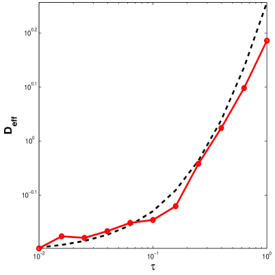
Figure 1: Effective diffusivity for (21b) with $V(x)=\cos(x)$ as a function of $\tau$, for $\sigma=1,\,D=\frac{k_{B}T}{\gamma}=1,\,\gamma=1$. Solid line: Results from Monte Carlo simulations. Dashed line: Results from formula (23).

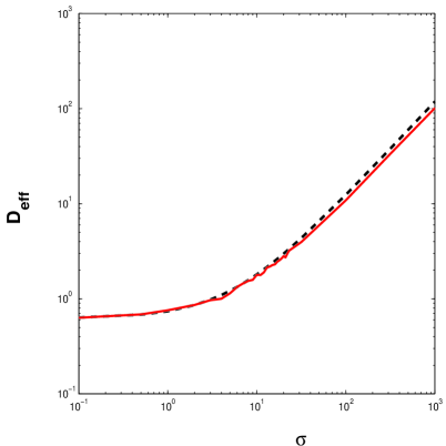
Figure 2: Effective diffusivity for (21b) with $V(x)=\cos(x)$ as a function of $\sigma$, for $\tau=0.1,\,D=\frac{k_{B}T}{\gamma}=1,\,\gamma=1$. Solid line: Results from Monte Carlo simulations. Dashed line: Results from formula (23).

In figure 1 we present the effective diffusion coefficient as a function of the correlation time $\tau$ of the OU process. We also plot the results of the small $\tau$ asymptotics. The agreement between theoretical predictions and numerical results is quite satisfactory, for $\tau\ll 1$. We also observe that the effective diffusivity is an increasing function of $\tau$.

In figure 2 we plot the effective diffusivity as a function of the noise strength $\sigma$ of the OU process. As expected, the effective diffusivity is an increasing function of $\sigma$. The agreement between the theoretical predictions from (23) and the numerical experiments is excellent.

5 Summary and Conclusions

The problem of Brownian motion in a periodic potential and driven by external forces was studied in this paper. Using multiscale techniques we derived formulae for the effective drift and the effective diffusion tensor. We used these formulae to calculate the effective diffusion coefficient for a Brownian particle in a one dimensional periodic potential which is driven by additive colored noise. The theoretical predictions are in very good agreement with the results obtained from direct numerical calculations.

In order to streamline the presentation, we studied the cases of Markovian and time–periodic external fluctuations separately. It is straightforward, of course, to combine the two and obtain formulae for the effective drift and the effective diffusion coefficient when some of the processes are random and some periodic. Furthermore, the case where the forcing terms depend on the particle position can be treated easily within the framework developed in this paper. In order for our method to be applicable in this case it is necessary for the fast process to be ergodic for all values of the state variable $x$. We believe, thus, that our multiscale approach is general enough to encompass essentially all models for periodic potentials and external fluctuations that have been considered within the framework of Brownian motors.

The multiscale technique employed in this paper provides us with a systematic method for analyzing the long time behavior of solutions to the stochastic equations of motion. The assumption of scale separation upon which the method is based is always satisfied for systems with a finite number of characteristic length and time scales. Naturally, the results of the multiscale analysis are valid at length and time scales large compared to the largest length and time scales of the system. For example, the time required for the correlation ratchet (21b) to reach its asymptotic Brownian regime increases as the correlation time $\tau$ increases. However, for finite $\tau$ the system will always eventually perform an effective Brownian motion.

In this paper we only presented formal calculations. We emphasize however that all the results presented in this paper can be justified rigorously, and in a very general setting. The key assumptions are the ergodicity of the fast process generated by ${\mathcal{L}}_{0}$, defined in (11), and the well–posedness of the Poisson equation (20). Ergodicity implies the existence of the effective drift: this is a consequence of the strong law of large numbers. Ergodicity, together with well–posedness of eqn. (20) imply the existence of the effective diffusion coefficient: this is a consequence of the martingale central limit theorem, see e.g. [10, ch. 7]. Needless to say, checking the ergodicity of the fast process and the well posedness of (20) are not trivial tasks. Results of this form are proved, for example, in [14].

In the case of stochastic external fluctuations, the calculation of the effective diffusion tensor requires the numerical solution of equations (12) and (20). It is conceivable that this task might be as computationally demanding as direct Monte Carlo simulations. From this point of view the main advantage of our approach is that it provides a natural starting point for careful asymptotic analysis and rigorous study of the dependence of the effective drift and the effective diffusion coefficient on the various parameters of the problem.

On the contrary, when the coefficients of eqn. (3) are periodic in time, the calculation of $D_{eff}$ requires the numerical solution of eqns. (30) and (37). These are PDEs with periodic coefficients and can be routinely solved with e.g. a spectral method. In this setting, our approach offers a clear computational advantage over Monte Carlo simulations. We also mention in passing that the various formulae for the effective diffusion coefficient that have been derived in the literature [12, 19, 32, 35] can be obtained from equation (36): they correspond to cases where equations (31) and (37) can be solved analytically. An example–the calculation of the effective diffusion coefficient of an overdamped Brownian particle in a tilted periodic potential–is presented in appendix. Similar calculations yield analytical expressions for all other exactly solvable models that have been considered in the literature.

In this paper we have studied the overdamped limit. There are various problems, however, where inertial effects are important and cannot be neglected. As examples we mention rocking ratchets in SQUIDS, [30, sec. 5.10], surface diffusion [18, 34], inertial particles [27, 14]. Our framework can be generalized to include inertial effects. It is very interesting, then, to understand the dependence of the effective diffusion coefficient on the particle inertia. This problem is currently under investigation.

Acknowledgements The author is indebted to Professors C.R. Doering and A.M. Stuart for useful discussions and suggestions.

Appendix A Time–Periodic Coefficients

In this appendix we derive formulae for the mean drift and the effective diffusion coefficient for a Brownian particle which moves according to

$$\gamma\dot{x}(t)=-\nabla V(x(t),t)+y(t)+\sqrt{2\gamma k_{B}T(x(t),t)}\xi(t),$$ (25)

for space–time periodic potential $V(x,t)$ and temperature $T(x,t)>0$, and periodic in time force $y(t)$. We take the spatial period to be $L$ in all directions and the temporal period of $V(x,t),\,T(x,t)$ and $y(t)$ to be $\mathcal{T}$. We use the notation $Q=[0,L]^{d}$. Equation (25) is interpreted in the Itô sense. This is the correct interpretation when eqn. (25) is obtained from the full phase space dynamics, in the limit as the inertia tends to $0$ [17, 26]. Since the analysis is very similar to the one presented in [3, 37] we will be brief.

A.1 Calculation of the Effective Drift

The backward Kolmogorov equation corresponding to (25) reads

$$\frac{\partial u(x,t)}{\partial t}=F(x,t)\cdot\nabla_{x}u(x,t)+\frac{k_{B}T(x,t)}{\gamma}\Delta_{x}u(x,t),$$ (26)

where $F(x,t)=\frac{1}{\gamma}(-\nabla V(x,y)+y(t))$. We re–scale space and time in (26) according to $x=\rightarrow\epsilon x,\,t\rightarrow\epsilon t$. We look for a solution of the resulting equation of the form

$$u^{\epsilon}(x,t)=u_{0}\left(x,\frac{x}{\epsilon},t,\frac{t}{\epsilon}\right)+\epsilon u_{1}\left(x,\frac{x}{\epsilon},t,\frac{t}{\epsilon}\right)+\epsilon^{2}u_{2}\left(x,\frac{x}{\epsilon},t,\frac{t}{\epsilon}\right)+\dots.$$ (27)

We treat $x,\,z=x/\epsilon$ and $t,\,\tau=t/\epsilon$ as independent variables. We emphasize that $u_{i}(x,z,t,\tau),\,i=0,1,2,\dots$ are periodic functions in both $z$ and $\tau$. Upon substituting (27) into (26), using the chain rule and equating the coefficients of equal powers in $\epsilon$ we obtain the following sequence of equations

$${\mathcal{R}}_{0}u_{0} = 0,$$ (28)

$${\mathcal{R}}_{0}u_{1} = -{\mathcal{R}}_{1}u_{0},$$ (29)

$$\dots = \dots,$$

where

$$\mathcal{R}_{0}=\frac{\partial}{\partial\tau}-{\mathcal{L}}_{0},\quad{\mathcal{L}}_{0}=F(z,\tau)\cdot\nabla_{z}+\frac{kT(z,\tau)}{\gamma}\Delta_{z}$$

and

$$\mathcal{R}_{1}=\frac{\partial}{\partial t}-{\mathcal{L}}_{1},\quad{\mathcal{L}}_{1}=F(z,\tau)\cdot\nabla_{x}+\frac{2k_{B}T(z,\tau)}{\gamma}\nabla_{z}\nabla_{x}.$$

The equation

$${\mathcal{R}}_{0}^{*}\rho(z,\tau)=\frac{\partial\rho(z,\tau)}{\partial\tau}+\nabla_{z}\left(F(z,\tau)\rho(z,\tau)\right)+\frac{k_{B}T(z,\tau)}{\gamma}\Delta_{z}\rho(z,\tau)=0,$$ (30)

with

$$\int_{0}^{\mathcal{T}}\int_{Q}\rho(z,\tau)\,dzd\tau=1$$

and periodic boundary conditions in both $z$ and $\tau$ has a unique solution under appropriate regularity assumptions on $F(z,t),\,T(z,t)$ [3, Thm. 3.10.1]. By Fredholm alternative, (28) implies that

$$u_{0}=u(x,t).$$

Eqn. (29) now becomes

$${\mathcal{R}}_{0}u_{1}=\frac{\partial u(x,t)}{\partial t}-F(z,\tau)\cdot\nabla_{x}u(x,t).$$

The solvability condition for this equation leads to the following backward Liouville equation

$$\frac{\partial u(x,t)}{\partial t}=U_{eff}\cdot\nabla_{x}u(x,t),$$

with

$$U_{eff}=\int_{0}^{\mathcal{T}}\int_{Q}F(z,\tau)\rho(z,\tau)\,dzd\tau=0.$$ (31)

A.2 Calculation of the Effective Diffusion Coefficient

Without loss of generality we assume that the effective drift given by (31) vanishes, $U_{eff}=0$. We perform the diffusive re–scaling in equation (26), $x\rightarrow\epsilon x,\,t\rightarrow\epsilon^{2}t$. We go through the same analysis as in the previous subsection to obtain the following sequence of equations.

$${\mathcal{R}}_{0}u_{0} = 0,$$ (32)

$${\mathcal{R}}_{0}u_{1} = -{\mathcal{L}}_{1}u_{0},$$ (33)

$${\mathcal{R}}_{0}u_{2} = -{\mathcal{L}}_{1}u_{1}-{\mathcal{L}}_{2}u_{0}$$ (34)

$$\dots = \dots,$$

where ${\mathcal{R}}_{0},\,{\mathcal{L}}_{0},\,{\mathcal{L}}_{1}$ were defined in the previous subsection and

$${\mathcal{L}}_{2}=\frac{\partial}{\partial t}-\frac{k_{B}T(z,\tau)}{\gamma}\Delta_{x}.$$

Equation (32) gives that $u_{0}=u(x,t)$. Equation (33) becomes

$${\mathcal{R}}_{0}u_{1}=-F(z,\tau)\cdot\nabla_{x}u(x,t).$$

Since we have assumed that $U_{eff}=0$, this equation is well posed. Its solution is

$$u_{1}(x,z,t,\tau)=\chi(z,\tau)\cdot\nabla_{x}u(x,t),$$

where

$$-{\mathcal{R}}_{0}\chi(z,\tau)=F(z,\tau).$$ (35)

The solvability condition for equation (34) reads

$$\int_{0}^{\mathcal{T}}\int_{Q}\left(-{\mathcal{L}}_{1}u_{1}-{\mathcal{L}}_{2}u_{0}\right)\,dzd\tau=0,$$

from which, after some algebra we obtain an evolution equation for $u(x,t)$

$$\frac{\partial u(x,t)}{\partial t}=\sum_{i,j=1}^{d}D_{ij}\frac{\partial^{2}u(x,t)}{\partial{x_{i}}\partial{x_{j}}}.$$

The effective diffusion coefficient is

$$D_{ij} = \delta_{ij}\frac{k_{B}}{\gamma}\langle T(z,\tau)\rangle_{\rho}+\langle F_{i}(z,\tau)\chi^{j}(z,\tau)\rangle_{\rho}$$ (36)

$$+\frac{2k_{B}}{\gamma}\left\langle T(z,\tau)\frac{\partial\chi^{i}(z,\tau)}{\partial y_{j}}\right\rangle_{\rho}$$

with

$$\langle\cdot\rangle_{\rho}=\int_{0}^{\mathcal{T}}\int_{Q}\cdot\rho(z,\tau)\,dzd\tau.$$

When $U_{eff}\neq 0$, eqns. (35) and (36) become, respectively,

$$-{\mathcal{R}}_{0}\chi(z,\tau)=F(z,\tau)-U_{eff}$$ (37)

and

$$D_{ij} = \delta_{ij}\frac{k_{B}}{\gamma}\langle T(z,\tau)\rangle_{\rho}+\langle\left(F_{i}(z,\tau)-U_{eff}^{i}\right)\chi^{j}(z,\tau)\rangle_{\rho}$$ (38)

$$+\frac{2k_{B}}{\gamma}\left\langle T(z,\tau)\frac{\partial\chi^{i}(z,\tau)}{\partial y_{j}}\right\rangle_{\rho}$$

Appendix B Effective Diffusion Coefficient for Tilted Periodic Potentials

In this appendix we use our method to obtain a formula for the effective diffusion coefficient of an overdamped particle moving in a one dimensional tilted periodic potential. This formula was first derived and analyzed in [32, 31] without any appeal to multiscale analysis. The equation of motion is

$$\dot{x}=-V^{\prime}(x)+F+\sqrt{2D}\xi,$$ (39)

where $V(x)$ is a smooth periodic function with period $L$, $F$ and $D>0$ constants and $\xi(t)$ standard white noise in one dimension. To simplify the notation we have set $\gamma=1$.

The stationary Fokker–Planck equation corresponding to(39) is

$$\partial_{x}\left(\left(V^{\prime}(x)-F\right)\rho(x)+D\partial_{x}\rho(x)\right)=0,$$ (40)

with periodic boundary conditions. Formula (13) for the effective drift now becomes

$$U_{eff}=\int_{0}^{L}(-V^{\prime}(x)+F)\rho(x)\,dx.$$ (41)

The solution of eqn. (40) is [29, Ch. 9]

$$\rho(x)=\frac{1}{Z}\int_{x}^{x+L}dyZ_{+}(y)Z_{-}(x),$$ (42)

with

$$Z_{\pm}(x):=e^{\pm\frac{1}{D}(V(x)-Fx)},$$

and

$$Z=\int_{0}^{L}dx\int_{x}^{x+L}dyZ_{+}(y)Z_{-}(x).$$ (43)

Upon using (42) in (41) we obtain [29, Ch. 9]

$$U_{eff}=\frac{DL}{Z}\left(1-e^{-\frac{F\,L}{D}}\right).$$ (44)

Our goal now is to calculate the effective diffusion coefficient. For this we first need to solve the Poisson equation (20) which now becomes

$${\mathcal{L}}\chi(x):=D\partial_{xx}\chi(x)+(-V^{\prime}(x)+F)\partial_{x}\chi=V^{\prime}(x)-F+U_{eff},$$ (45)

with periodic boundary conditions. Then we need to evaluate the integrals in (18):

$$D_{eff}=D+\int_{0}^{L}(-V^{\prime}(x)+F-U_{eff})\rho(x)\,dx+2D\int_{0}^{L}\partial_{x}\chi(x)\rho(x)\,dx.$$

It will be more convenient for the subsequent calculation to rewrite the above formula for the effective diffusion coefficient in a different form. The fact that $\rho(x)$ solves the stationary Fokker–Planck equation, together with elementary integrations by parts yield that, for all sufficiently smooth periodic functions $\phi(x)$,

$$\int_{0}^{L}\phi(x)(-{\mathcal{L}}\phi(x))\rho(x)\,dx=D\int_{0}^{L}(\partial_{x}\phi(x))^{2}\rho(x)\,dx.$$

Now we have

$$D_{eff} = D+\int_{0}^{L}(-V^{\prime}(x)+F-U_{eff})\chi(x)\rho(x)\,dx+2D\int_{0}^{L}\partial_{x}\chi(x)\rho(x)\,dx$$ (46)

$$= D+\int_{0}^{L}(-{\mathcal{L}}\chi(x))\chi(x)\rho(x)\,dx+2D\int_{0}^{L}\partial_{x}\chi(x)\rho(x)\,dx$$

$$= D+D\int_{0}^{L}\left(\partial_{x}\chi(x)\right)^{2}\rho(x)\,dx+2D\int_{0}^{L}\partial_{x}\chi(x)\rho(x)\,dx$$

$$= D\int_{0}^{L}\left(1+\partial_{x}\chi(x)\right)^{2}\rho(x)\,dx.$$

Now we solve the Poisson equation (45) with periodic boundary conditions. We multiply the equation by $Z_{-}(x)$ and divide through by $D$ to rewrite it in the form

$$\partial_{x}(\partial_{x}\chi(x)Z_{-}(x))=-\partial_{x}Z_{-}(x)+\frac{U_{eff}}{D}Z_{-}(x).$$

We integrate this equation from $x-L$ to $x$ and use the periodicity of $\chi(x)$ and $V(x)$ together with formula (44) to obtain

$$\partial_{x}\chi(x)Z_{-}(x)\left(1-e^{-\frac{F\,L}{D}}\right)=-Z_{-}(x)\left(1-e^{-\frac{F\,L}{D}}\right)+\frac{L}{Z}\left(1-e^{-\frac{F\,L}{D}}\right)\int_{x-L}^{x}Z_{-}(y)\,dy,$$

from which we immediately get

$$\partial_{x}\chi(x)+1=\frac{1}{Z}\int_{x-L}^{x}Z_{-}(y)Z_{+}(x)\,dy.$$

Substituting this into (46) and using the formula for the invariant distribution (42) we finally obtain

$$D_{eff}=\frac{D}{Z^{3}}\int_{0}^{L}(I_{+}(x))^{2}I_{-}(x)\,dx,$$ (47)

with

$$I_{+}(x)=\int_{x-L}^{x}Z_{-}(y)Z_{+}(x)\,dy\quad\mbox{and}\quad I_{-}(x)=\int_{x}^{x+L}Z_{+}(y)Z_{-}(x)\,dy.$$

Formula (47) for the effective diffusion coefficient (formula (22) in [31]) is the main result of this appendix.

References

- [1] A. Barone and G. Paterno. Physics and Applications of the Josephson Effect. Wiley, New York, 1982.
- [2] R. Bartussek, P. Reimann, and P. Hanggi. Precise numerics versus theory for correlation ratchets. Phys. Rev. Let., 76(7):1166–1169, 1996.
- [3] A. Bensoussan, J.L. Lions, and G. Papanicolaou. Asymptotic analysis of periodic structures. North-Holland, Amsterdam, 1978.
- [4] M. Bier and R.D. Astumian. Biasing Brownian motion in different directions in a 3–state fluctuating potential and application for the separation of small particles. Phys. Rev. Let., 76(22):4277, 1996.
- [5] C. Bustamante, D. Keller, and G. Oster. The physics of molecular motors. Acc. Chem. res., 34:412–420, 2001.
- [6] I. Derenyi, , and R.D. Astumian. ac separation of particles by biased Brownian motion in a two–dimensional sieve. Phys. Rev. E, 58(6):7781–7784, 1998.
- [7] C.R. Doering, L. A. Dontcheva, and M.M. Klosek. Constructive role of noise: fast fluctuation asymptotics of transport in stochastic ratchets. Chaos, 8(3):643–649, 1998.
- [8] C.R. Doering, W. Horsthemke, and J. Riordan. Nonequilibrium fluctuation–induced transport. Phys. Rev. Let., 72(19):2984–2987, 1994.
- [9] R. Eichhorn and P. Reimann. Paradoxical directed diffusion due to temperature anisotropies. Europhys. Lett., 69(4):517–523, 2005.
- [10] S.N. Ethier and T.G. Kurtz. Markov processes. Wiley Series in Probability and Mathematical Statistics: Probability and Mathematical Statistics. John Wiley & Sons Inc., New York, 1986.
- [11] P. Fulde, L. Pietronero, W. R. Schneider, and S. Strässler. Problem of brownian motion in a periodic potential. Phys. Rev. Let., 35(26):1776–1779, 1975.
- [12] H. Gang, A. Daffertshofer, and H. Haken. Diffusion in periodically forced Brownian particles moving in space–periodic potentials. Phys. Rev. Let., 76(26):4874–4877, 1996.
- [13] C. W. Gardiner. Handbook of stochastic methods. Springer-Verlag, Berlin, second edition, 1985. For physics, chemistry and the natural sciences.
- [14] M. Hairer and G. A. Pavliotis. Periodic homogenization for hypoelliptic diffusions. J. Stat. Phys., 117(1/2):261–279, 2004.
- [15] W. Horsthemke and R. Lefever. Noise-induced transitions, volume 15 of Springer Series in Synergetics. Springer-Verlag, Berlin, 1984. Theory and applications in physics, chemistry, and biology.
- [16] C. Kipnis and S. R. S. Varadhan. Central limit theorem for additive functionals of reversible Markov processes and applications to simple exclusions. Comm. Math. Phys., 104(1):1–19, 1986.
- [17] R. Kupferman, G. A. Pavliotis, and A.M. Stuart. Itô versus Stratonovich white noise limits for systems with inertia and colored multiplicative noise. Phys. Rev. E, 70:036120, 2004.
- [18] A.M. Lacasta, J.M Sancho, A.H. Romero, I.M. Sokolov, and K. Lindenberg. From subdiffusion to superdiffusion of particles on solid surfaces. Phys. Rev. E, 70:051104, 2004.
- [19] S. Lifson and J.L. Jackson. On the self–diffusion of ions in polyelectrolytic solution. J. Chem. Phys, 36:2410, 1962.
- [20] B. Lindner, M. Kostur, and L. Schimansky-Geier. Optimal diffusive transport in a tilted periodic potential. Fluctuation and Noise Letters, 1(1):R25–R39, 2001.
- [21] M. O. Magnasco. Forced thermal ratchets. Phys. Rev. Let., 71(10):1477–1481, 1993.
- [22] J.C. Mattingly and A. M. Stuart. Geometric ergodicity of some hypo-elliptic diffusions for particle motions. Markov Processes and Related Fields, 8(2):199–214, 2002.
- [23] B. Oksendal. Stochastic Differential Equations. Springer-Verlag, Berlin-Heidelberg-New York, 1998.
- [24] G. C. Papanicolaou. Introduction to the asymptotic analysis of stochastic equations. In Modern modeling of continuum phenomena (Ninth Summer Sem. Appl. Math., Rensselaer Polytech. Inst., Troy, N.Y., 1975), pages 109–147. Lectures in Appl. Math., Vol. 16. Amer. Math. Soc., Providence, R.I., 1977.
- [25] G.C. Papanicolaou. Asymptotic analysis of stochastic equations. In Studies in probability theory, volume 18 of MAA Stud. Math., pages 111–179. Math. Assoc. America, Washington, D.C., 1978.
- [26] G. A. Pavliotis and A.M. Stuart. Analysis of white noise limits for stochastic systems with two fast relaxation times. SIAM J. MMS, 4(1):1–35, 2005.
- [27] G. A. Pavliotis and A.M. Stuart. Periodic homogenization for inertial particles. Physica D, 204(3–4):161–187, 2005.
- [28] H. Qian, Min Qian, and X. Tang. Thermodynamics of the general duffusion process: time–reversibility and entropy production. J. Stat. Phys., 107(5/6):1129–1141, 2002.
- [29] R. L. R. L. Stratonovich. Topics in the theory of random noise. Vol. II. Revised English edition. Translated from the Russian by Richard A. Silverman. Gordon and Breach Science Publishers, New York, 1967.
- [30] P. Reimann. Brownian motors: noisy transport far from equilibrium. Phys. Rep., 361(2-4):57–265, 2002.
- [31] P. Reimann, C. Van den Broeck, H. Linke, P. Hänggi, J.M. Rubi, and A. Perez-Madrid. Diffusion in tilted periodic potentials: enhancement, universality and scaling. Phys. Rev. E, 65(3):031104, 2002.
- [32] P. Reimann, C. Van den Broeck, H. Linke, J.M. Rubi, and A. Perez-Madrid. Giant acceleration of free diffusion by use of tilted periodic potentials. Phys. Rev. Let., 87(1):010602, 2001.
- [33] H. Risken. The Fokker-Planck equation, volume 18 of Springer Series in Synergetics. Springer-Verlag, Berlin, 1989.
- [34] J.M Sancho, A.M. Lacasta, K. Lindenberg, I.M. Sokolov, and A.H. Romero. Diffusion on a solid surface: anomalous is norms. Phys. Rev. Let, 92(25):250601, 2004.
- [35] M Schreier, P. Reimann, P. Hänggi, and E. Pollak. Giant enhancement of diffusion and particle selection in rocked periodic potentials. Europhys. Let., 44(4):416–422, 1998.
- [36] T.C.Elston and C.R. Doering. Numerical and analytical studies of nonequilibrium fluctuation-induced transport processes. J. Stat. Phys., 83:359–383, 1996.
- [37] M. Vergassola and M. Avellaneda. Scalar transport in compressible flow. Phys. D, 106(1-2):148–166, 1997.