Probing the intrinsic shot noise of a Luttinger Liquid through impedance matching.
Abstract
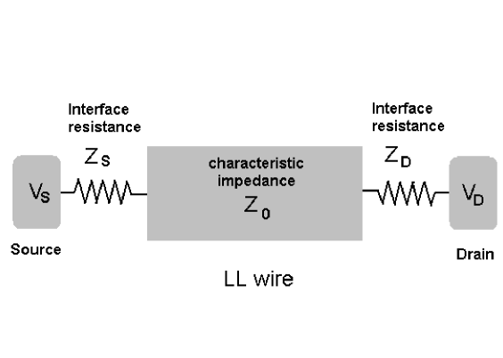
We argue that a simple way to bypass reflections at the boundaries of a finite Luttinger liquid (LL) connected to electrodes is to match load and drain impedances to the characteristic impedance of the LL viewed as a mesoscopic transmission line.
For an impedance matched LL, this implies that the AC and DC shot noise properties of a finite LL are identical to those of an infinite LL.
Even for an impedance mismatched LL, we show by a careful analysis of reflections that the intrinsic infinite LL properties can still be extracted yielding possibly irrational charges for the LL elementary excitations. We improve on existing results for AC shot noise by deriving expressions with explicit dependence on the charges of the fractional states. Most notably these results can be established quite straightforwardly without resort to the Keldysh technique.
We apply these arguments to two experimental setups which allow the observation of different sets of fractional quasiparticles: (i) injection of current by a STM tip in the bulk of a LL; (ii) backscattering of current by an impurity.
I Introduction.
Shot noise is a topic of current interest because it allows access to non-equilibrium transport properties of a system and notably to the charge carried by the elementary excitations noise . For a standard non-disordered Fermi liquid shot noise yields a unit charge for the Landau quasiparticle but in the Fractional Quantum Hall Effect (FQHE) shot noise has revealed rational charges for the famous Laughlin quasiparticles fqhe .
The Luttinger liquid ll is another example of strongly-correlated system where elementary excitations with non-integral charges are expected. While the standard bosonization picture of the LL stresses plasmon-like excitations and zero modes bosonisation , that picture is unconvenient to interpret shot noise because the charged excitations have no dynamics (they are zero-modes with no dispersion); an alternative ’fractional states picture’ of the charged excitations was recently developped fractionalization : it was shown that there are other bases of exact eigenstates for the LL consisting of states carrying in general irrational charges (a summary will be found in Appendix A). The fractional states are created in pairs with a total charge which is always an integer.
These fractional eigenstates permit a straight interpretration of earlier shot noise results for an infinite LL with an impurity, where a charge was found in the shot noise kane ( is the usual LL parameter). A very recent calculation for the shot noise due to current injection by a STM tip in an infinite LL also found that charges and are involved stm . States with such unconventional charges are difficult to account with in the standard bosonized picture of the LL while they come out naturally in the ’fractional states picture’ of the LL, where they had earlier been predicted and built as exact eigenstates of the LL hamiltonian fractionalization .
In spite of these theoretical results for the shot noise great strides are still needed toward an experimental verification for the following reason: the experimental systems have a finite length and are mostly at the mesoscopic scale, which makes it impossible to ignore the influence of electrodes on the transport properties of the LL. Theorists have therefore been busy trying to model reservoirs and compute conductance as well as current fluctuations for the LL: it is now accepted that the conductance of the finite LL connected to two electrodes differs from the conductance of the infinite LL ill . Shot noise has also been computed by several groups for the following setups: (i) STM tip injecting current stm ; (ii) backscattering due to an impurity impurity ; pono , and claims have been made that charges of fractional excitations can be recovered from AC shot noise.
However several criticisms can be addressed to those claims:
- (a) the calculations depend on a very specific model, the inhomogeneous LL which models electrodes as 1D free fermions ill , which is a debatable assumption; to what extent these calculations are sufficiently general and model-independent is hard to assess.
- (b) Both the charge of fractional excitations and the reflection parameter used in these models depend on the LL parameter : but the Fano factor mixes contributions from both the fractional charge and the reflection parameter; this implies that a measurement of the Fano factor reduces to just measuring the LL parameter and is not a direct measurement of the charge of the charge-carriers (contrast eq.(68) with our results, e.g. eq.(73) ). In the case of an impurity in a LL the AC Fano factor is a periodic function with period (for the unlikely case of an impurity sitting exactly in the middle of the LL) and it was claimed impurity that averaging over one period yields the fractional charge : it is difficult to understand why it should be so and actually as we will show in this paper this result is a model-dependent accident and in general averaging over a period does NOT yield the charge of the fractional excitation of the LL.
We use in this paper a general formalism encompassing the inhomogeneous LL and can thus address these qualms:
- (a) we indeed showed in several earlier papers that the inhomogeneous LL is actually curtailed to very specific experimental conditions (interface resistances of the LL to the electrodes pinned at half-a-quantum of resistance ): it is a special case of our theory, which is itself valid for arbitrary values of the interface resistances at the electrodes p3 .
- (b) our theory for a LL in a multi-terminal environment has the advantage of being able to sort out from the Fano factor the contributions coming from reflections and those coming from the fractional charges. As a result it does show unambiguously how to get access to the fractional charges.
To perform shot noise calculations a tool of choice is of course the Keldysh technique. That approach can also be used within our framework (and is sketched in Appendix B). However in the finite geometry in the course of the Keldysh calculation the distinction between the dual role of the LL parameter (which intervenes both in the charges scattered and in the reflection coefficients) is blurred so that the difficulties explained above apply (point (b) ). We follow another route in this paper and show the essential physics (and almost all of the earlier results found with the inhomogeneous LL) can be retrieved from a fine analysis of reflections and from viewing the LL as a mesoscopic transmission line.
More importantly such an approach yields insights on how to bypass the effect of reflections, which (although yielding an interesting physics in themselves), are largely a nuisance as far as measuring the fractional charges is concerned: to avoid reflections in a transmission line it is sufficient to match the load and drain impedances to the characteristic impedance of the line. As a result the system behaves as if it were an infinite system. The AC shot noise properties of an impedance matched LL are therefore exactly those of an infinite system.
The outline of the paper will be as follows:
- Section II is centered on the concept of impedance matching for a LL. It will introduce notations, explain the formalism used to describe the LL connected to reservoirs; that formalism makes use of boundary conditions describing quite straightforwardly the coupling of a LL to interface resistances. This assumes ohmic coupling of the LL to electrodes. The section concludes with the proof that the impedance matched LL is equivalent to an infinite LL.
- Section III discusses the setup of a STM tip injecting electrons in a LL and generalizes results found within the framework of the inhomogeneous LL.
- Section IV shows how to use calculations done for the STM tip setup to infer AC shot noise for another apparently unrelated setup, that of an impurity which backscatters current in a LL. We again generalize the inhomogeneous LL results.
II Impedance matching.
II.1 LL as a mesoscopic transmission line.
The LL is just a quantum LC line as evidenced from its hamiltonian:
where is the difference between bare right and left electron densities (at right and left Fermi points ). Rewriting the Hamiltonian in terms of charge density and current:
(the last expression follows from charge conservation and the equations of motion) there follows:
which shows the LL has both capacitance and inductance per unit length:
These capacitive and inductive behaviours show up quite well in the LL dynamical conductance and dynamical impedance as computed in Ref. p3 .
II.2 Basics of transmission lines: Impedance mismatch.
As for any finite transmission line (or for that matter, any sound wave in a tube, etc…) for the open system (rigid boundaries) one has standing waves due to perfect reflection at the boundaries.
Such a transmission line is characterized by a characteristic impedance
| (1) |
We remind the reader that a characteristic impedance IS NOT a standard DC or AC impedance: it is rather an instantaneous or surge impedance seen by the electrical wave as it moves along the LC line. The stark difference can be seen for example for a resistanceless LC line: the DC impedance is then zero while the characteristic impedance is non-zero. For the usual LC line obeys:
where the total voltage signal is and are right (or left) moving currents so that .
If one now attaches load impedances and at the interfaces of a length transmission line such that:
| (2) |
freshman physics tells us also that there will be reflection at the boundaries and with respectively reflexion coefficients (for the plasma wave):
| (3) |
This implies that reflexions are killed whenever the load impedances at the source and drain are equal to the characteristic impedance. This leads to the concept of impedance matching well-known to electrical engineers: by carefully matching the load impedances one eliminates undesired reflections and one can thus have a maximal energy transfer from source to load.
Furthermore for load impedances attached to a resistanceless transmission line one has a series addition law and therefore:
| (4) |
II.3 Formalism used in this paper: ’impedance boundary conditions’.
We will use a description of the LL connected to reservoirs p3 which is the exact implementation of the customary load impedances boundary conditions described in the previous subsection and used for transmission lines or sound waves in tubes:
| (5) | |||||
| (6) |
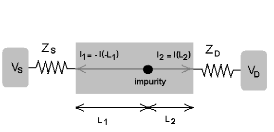
and are interface impedances at respectively the source and the drain which for simplicity will be assumed to be real numbers throughout the paper (but more general situations could be discussed), is the current operator, and source and drain are set at a voltage or (see Fig.1). The Heisenberg picture is assumed so that we work with time-dependent operators. Since is the energy needed to add locally a particle, it corresponds to a local chemical potential for the LL. Actually the boundary conditions are tantamount to assuming Ohm’s law at the boundaries of the system: the current is proportional to a voltage drop between the reservoir and the LL wire and the proportionality constant is just an interface resistance.
For calculations it is convenient to introduce chiral chemical potentials corresponding to the chiral plasmons of the LL.
We consider the standard Luttinger Hamiltonian for a wire of length .
| (7) |
and are chiral particle densities which obey the relation . Their sum is just the total particle density while the electrical current is simply .
We now define the following operators:
| (8) |
Physically they correspond to chemical potential operators: their average value yields the energy needed to add one particle at position to the chiral density: . These chiral chemical potentials correspond to the plasma chiral eigenmodes of the Luttinger liquid and not to the left or right moving (bare) electrons.
| (10) | |||||
Since these operators have a chiral time evolution:
| (11) |
it follows also:
| (12) | |||||
| (13) |
where we have defined a plasmon phase accumulated along the wire as:
| (14) |
II.4 DC conductance of the impedance mismatched system.
This section is mostly present for pedagogical reasons. We first review the derivation of the DC conductance in this formalism (earlier discussion can be found in p1 and p2 ). We will then show how the calculation is interpreted in terms of reflections of the plasma wave; this provides a simple context which will help us later when we seek to interpret this paper’s results on the shot noise.
II.4.1 A straight derivation.
The boundary conditions can be rewritten in terms of the chiral chemical potentials as:
| (15) |
In the DC regime these operators lose their space and time-dependence therefore adding the two previous equations yield: . The DC conductance is thus:
as expected for a resistanceless LC-line connected in series to two load impedances. For the impedance matched system:
and therefore using eq.(1):
which is exactly the DC conductance of the infinite system kcond .
The same considerations can be applied to the AC conductance matrix p3 and one finds that the impedance-matched system has exactly the properties of the infinite system.
II.4.2 Physical interpretation: an equivalent derivation using reflections.
As seen in the previous subsection the computation of the DC conductance is quite straightforward using the ’impedance boundary conditions’. For the sake of pedagogy we will rederive the DC conductance as a function of reflection coefficients.
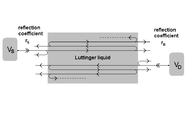
We consider for full generality arbitrary reflections coefficients at the source and drain and . The source and drain are set at voltages and . We now build the contributions to the current resulting from the multiple reflections.
Order zero:we start with the values in the infinite system for the chiral currents injected by source and drain (see for instance key-5 ) as resulting from a straightforward linear-response calculation:
which yields . Resulting for the infinite system to a conductance renormalized by interactions: .The exponent corresponds to the chirality (right or left moving plasmons).
Order one: we take into account the reflections at the boundaries. This implies additional currents:
Each current has two contributions at this order: the first one corresponds to the reflexion at the boundary of the current of opposite chirality while the second one takes into account the fact that a fraction of the incoming current does not actually enter the system due to reflexion.
Order :
We have multiple reflexions of the chiral currents within the system. Therefore one simply has:
Let us now collect each contribution to get the total current.
Thus:
and the conductance is:
| (16) |
What do we learn from this calculation?
- (i) the multiple reflections are indeed not innocuous: they are at the heart of the renormalization of the conductance.
- (ii) for arbitrary values of the reflection coefficients the conductance can take any value.
- (iii) for reflection coefficients equal to zero one recovers the infinite system physics.
The third point may sound like a tautology but to radiowave engineers used to transmission lines this is but a statement of impedance matching, a concept whose importance has yet been unrecognized for the LL and the central issue of this paper.
-(iv) Let’s make contact with the ’impedance boundary conditions’, which can be rewritten as:
The values of the reflection coefficients can then be recovered; of course as expected from the analogy to a classical LC-transmission line one finds:
This is unsurprising given that the LL hamiltonian is quadratic and that therefore the classical equations of motion are exact.
Plugging in these values of the reflection coefficients into the expression of the conductance above ( eq.(16) ) one recovers as it should be:
II.5 Relation to the inhomogeneous LL and other models of a LL connected to leads.
The significance of reflections for a LL connected to leads was first recognized using the inhomogeneous LL, which is a model using a space dependent LL parameter: for and for for Fermi liquid leads ill .
It can be shown (see Appendix of Ref. p3 ) that the inhomogeneous LL and several other theories based on boundary conditions (such as the ’radiative boundary conditions’ key-6 ) actually obeys our ’impedance boundary conditions’ albeit in a very specific case, when load and drain impedances take the values:
These earlier theories will therefore be valid only for rather clean contacts with impedances close to those of a non-interacting system. Our more general approach has the advantage of not making such assumptions.
II.6 Proof that the impedance matched LL is equivalent to an infinite LL.
The proof is simple: the impedance matched LL is equivalent to an infinite LL because the Green’s function of a LL subjected to the ’impedance boundary conditions’ is identical with that of an infinite LL provided (impedance matching condition).
The Green’s function will not be used in this paper and the reader will find details in Appendix B which sketches its derivation. This is the starting point for a Keldysh treatment using the ’impedance boundary conditions’.
III Injection of particles through a STM tip.
In this section we discuss the following setup: a STM tip tunneling electrons into the bulk of a LL.
The obvious strategy to tackle the transport properties is to use the Keldysh formalism, which is well suited to non-equilibrium physics: this is the approach followed by Crépieux, Martin et coll., stm using the inhomogeneous LL. Actually the same can be done with the ’impedance boundary conditions’ ; the main difference is that the Green functions of the inhomogeneous LL correspond to the special case and that one has two reflection coefficients (at source and drain) instead of a single one. That approach is sketched in APPENDIX B.
We will show another more economical and physically more transparent approach which yields most of the physics (and often gives the same results). It is based upon making a distinction between operators for the injected currents and operators for the measured current.
We discuss separately DC and AC shot noise because our approach is simpler to understand in the DC case; additionally:
- for the DC noise, we discuss both asymetric injection of particles (unequal probability to inject an electron either at the left or the right Fermi point) and arbitrary interface resistances (in contrast Ref. stm deals with symetric injection and implies interface resistances set to ).
- for AC noise while keeping arbitrary interface resistances (which is the required setting for a discussion of impedance matching) we restrict for simplicity to symetric injection.
We also restrict ourselves in what follows to ’excess noise’ and never discuss ’equilibrium noise’ since the latter is in some sense trivial as it obeys the fluctuation-dissipation theorem.
III.1 DC shot noise.
Our derivation of the DC shot noise wil follow these steps:
- we first relate the current operators to another set of operators (’injected curent operators’)(section III.1.2);
- we compute the excess noise of these operators (section III.1.4);
- and finally infer from them the current excess noise (section III.1.5).
III.1.1 Earlier results
We consider the following apparatus: an STM tip tunnels electrons to the bulk of a LL (say, a carbon nanotube).
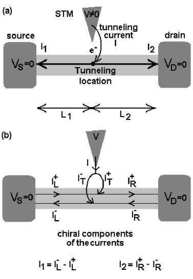
We call and the currents going to the left and to the right of the injection point. These currents are oriented OUTgoing from the injection point. They are the currents measured respectively at the source and drain. The main work on the subject is that of Crépieux, Martin and coll stm . They find that in the infinite system the direct correlations of current and cross-correlations obey:
where are the (in general irrational) charges of two fractional states: injection of a electron was proved to result in the creation of two exact fractional eigenstates of the LL fractionalization propagating in the right and left directions and carrying just such charges . (Injection of a electron results in the opposite: propagation to the left of charge and propagation to the right of charge ). These peculiar states are a combination of one Laughlin quasiparticle with one holon. A noteworthy observation is that Crépieux et al stm , find POSITIVE cross-correlations which is quite unexpected for a fermionic system.
(As an aside we note that such charges were anticipated in key-3 , where as a quantum average a charge density was found to separate into two charge packets carrying exactly the charges ; it was realized later in fractionalization that these charges are actually carried by exact fractional eigenstates).
Lebedev et al stm later found that these results were invalidated when the LL is connected to Fermi liquid reservoirs; one gets up to order two in perturbation:
So one recovers integral charges. This disappointing result is explained by Lebedev et al. as follows stm : in a second-order perturbation theory one neglects correlation between the transport of two electrons injected sequentially; assuming perfect transmission of the electron, a single injected electron will be transmitted as a whole to either one of the reservoirs so that which results into . As can one can see a crucial element of such an argumentation is perfect transmission of the injected electron. We will show in the course of this paper that such a condition can be relaxed (it actually depends crucially on the impedances at the boundaries of the system) which results in different values of the current-current correlators predicted by Crépieux, Martin and coll. stm .
(NB: As a shorthand notation we have written in the above the current correlation for the zero frequency Fourier transform of that quantity. We will also use this notation in the rest of the paper.)
III.1.2 Injected currents versus measured currents.
(We work here in the Heisenberg picture for the operators. Since we consider actually in this subsection a DC context the time dependence will be dropped.)
The goal of that subsection is to show that the operators for the measured currents and are NOT the operators for the currents and injected by the STM tip. The reason for that is simple: there are reflections at the boundaries. Imagine for instance that the STM tip injects current only to the left of the tip. Due to reflections eventually there must be some current flowing to the right which shows that the net currents and flowing in the system differ from the currents injected by the tip.
The rationale for making such distinctions is that the noise properties of and can be easily found and that from them the correlators for and can then be inferred very simply without recourse to the Keldysh technique.
Let us see that in detail.
Firstly we note that in this DC context the operators will have no space or time dependence; but due to the presence of the tunneling point we must distinguish the values of the operators to the left or to the right of the STM tip. Accordingly we note:
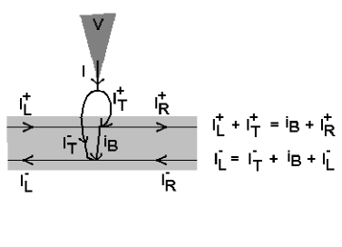
As we can see from Fig. 3 the operators for the current flowing to the left and to the right of the STM tip and the operators for the currents injected are different; by definition and using eq.(10),
where:
is the current carried by each chiral branch on the right (index ) or the left (index ) of the tunnelling tip (see Fig.2 (b) ). In other words what we call and are just the currents flowing in the wire.
In contrast the operators for the currents injected by the STM tip to its right and to its left are respectively:
The reason for that is that the eigenmodes of the LL are NOT left or right moving electrons: the current injected by the tip really goes into the chiral (plasmon) eigenmodes of the LL.
In the infinite system that discrepancy between injected and measured currents is irrelevant (for DC measurements) because for a LL wire which is grounded obviously since no current is coming from the electrodes: as a result and .
Not so in a finite geometry: there are of course reflections at the boundaries.
It is possible to relate the two sets of operators , and , . The special case of quantized resistances was previously discussed by the author and collaborators in p1 .
Using their definition one has in particular that the total tunneling current is:
We now use the boundary conditions, eq.(15) :
where the source and drain voltages have been set to the ground in this geometry; we have also used the fact that the operators are uniform.
This implies:
Finally:
| (25) | ||||
| (32) |
We stress that these relations hold very generally: the tunnel currents need not be small; the range of validity extends from the weak tunneling to the strong tunneling regime.
Essential remarks:
- (i) We recover the intuitively expected result that IF impedance matching is realized at BOTH boundaries, namely:
Then the measured currents and the injected currents are identical:
This gives the physical meaning of the injected current operators and : they would be the current operators if the system were infinite. This means that we can view the relation between the operators for the injected currents and and the operators for the measured currents , as an operator renormalization when one goes from the infinite system to the finite-length system.
- (ii) Why is it useful to consider the operators and ? Because in the DC regime by making some reasonable assumptions (Poisson injection by the STM tip) the Fano ratios are quite easy to find: actually they are identical with those of the infinite system, which is not quite unreasonable given the fact that and are just the current operators of the impedance-matched system.
For AC excess noise the correlators for and are not so easily found. But still we will find that assuming that their correlators are unchanged from their values in the infinite system yields the dominant behaviour for the excess noise for the measured currents , .
III.1.3 Physical interpretation : reflections.
The renormalization from and to and physically results from multiple reflections back and forth at the boundaries. This is a completely classical effect as seen for instance in waveguides, sound waves in a tube, etc, whenever load impedances are connected to the boundaries of the system and whenever there is an impedance mismatch.
Since this relation is the building-block of this paper for the sake of pedagogy we will now show how it can be recovered by directly considering reflections of the plasma wave. Let us define reflections coefficients and .
The plasma wave has two chiral components on the left and on the right of the impurity . We will build these currents sequentially.
Order zero:
If we take no account of the reflections then at zero order in a development in the reflection coefficients:
Order one:
The second line follows just from current conservation.
Order :
Therefore for :
and for :
Defining we have: later we will physically interpret some of this paper’s results for the shot noise through similar heuristic reasonings
and
Since and straightforward calculations lead to:
Comparison with the results found above:
shows they are identical provided one identifies
which is just the expression expected for e.g. a sound wave in a tube terminated by two load impedances!
This shows that the renormalizations of the tunneling currents follow simply from multiple reflections at the boundaries of the Luttinger liquid. Observe again that the origin of the phenomenon is purely classical and has no quantum grounds.
III.1.4 Excess noise for and for an STM with asymetric injection.
There are two processes for the injection: either (i) injection of an electron at or (ii) injection at .
As shown in fractionalization these electrons split in the LL and fractional eigenstates are created so that physically one injects the charges
in each arm: process (i) injection at : to the right and to the left; process (ii): to the right and to the left.
The total number of injections by either processes obeys Poisson statistics: we will work in a weak transmission limit (the current injected goes as a power law of the voltage difference between the electrode tip and the nanotube). We define the probabilities that a given injection is by process (ii) rather than (i) by . Microscopically we write the usual Luttinger hamiltonian plus a tunneling hamiltonian:
is the electron operator for an electron at the right Fermi point and is the electron operator for an electron at the left Fermi point ; is the creation operator for an electron in the electrode. We have allowed for distinct probability amplitudes for the injection of left and right electrons for full generality. The probabilities and are then simply:
is therefore the probability that a given charge injection is done with a left Fermi point electron rather than with a right Fermi electron.
As already emphasized by Crépieux et al, stm injection in a LL through an STM tip works as a Hanbury-Brown and Twiss device. Some care is however needed in the comparison: in a standard Hanbury-Brown and Twiss setting a source signal is partitioned with a probability to be transmitted and a probability of reflection; here for the LL what plays the role of the partitioning is the fact that an electron can be injected at either or : it is not the splitting of charge into fractional charges which acts as a partitioning. Choosing an asymetric STM electrode allows a better comparison to the Hanbury-Brown and Twiss setting since the probabilities and are not fixed at the value as in a symetric electrode. In the present experimental state of the art it may sem far-fetched to realize selective or asymetric injection of electrons but it might be feasible in a foreseeable future in quantum wires.
If the total number of injections is :
since we have assumed Poissonian statistics for the total number of electron injections. We call and the number of injections by respectively process (ii) or (i) above. Evidently one has the partition noise result (Burgess variance theorem):
Now using the assumption that the total number of injections obeys Poisson statistics, one finds that:
We infer the charge transmitted to the left of the tip (arm ), the current injected in the left arm and its fluctuations:
| (33) | ||||
| (34) |
And likewise in the right arm (arm ):
| (35) | ||||
| (36) |
The cross correlations follow easily:
| (37) |
We observe in passing that they are positive a fact already pointed out in stm for the special case of symetric injection. All those straightforward results can of course be recovered by a lengthier route through the Keldysh technique following Crépieux et al.
We stress furthermore that these relations are valid whether the LL wire is finite or not. Although the exact values of the correlators and of the current averages depend on the length of the system (the quantum average being taken over the length-dependent ground state) the Fano ratios are clearly invariant. In particular this means that the Fano ratios for the injected currents are exactly those of the measured currents and in the infinite system.
III.1.5 Excess noise for the measured currents: a mixing of direct and cross-correlations as compared to the infinite system.
Since :
it follows that the DC noise correlations for the measured currents are:
| (39) | ||||
| (41) | ||||
| (42) |
where are the correlators of the injected currents.
Since the Fano factors for are identical to those of and in the infinite system this shows that in the presence of boundaries there is a mixing of what would be in the infinite system the direct and cross correlations.
| (43) |
The latter equations then imply that (using eq.(32) ):
| (48) | ||||
| (51) |
Gathering eq.(32) and eq.(39) one then finds immediately:
and plugging the expression of the current injected to the left in function of the total current from eq.(43):
or in terms of the currents in each branch (using eq.(48) above):
| (52) |
which is the main result of the section.
Up to now we stress that the exact values of the charges and of the fractional states have not been used in the calculations: this implies that the set of equations eq.(52) can be used to extract experimentally their values EVEN in the absence of impedance matching ONCE the values of the load impedances and and the characteristic impedance are known through any transport measurement (time domain reflectometry, DC or AC conductance, etc…). Since one has three correlators, the experimental measurement of two of them should in principle allow for an extraction of the two charges and by fitting their values while the measurement of the third correlator (e.g. the cross-correlation) then becomes a distinct non-trivial prediction of the theory WITHOUT any fit.
However such a straightforward approach faces us with one conceptual issue: if we use the distinct predictions of the LL theory fractionalization ; p3 the characteristic impedance and the charges and are found not to be independent since:
If we plug in these values in the expression for the current correlators one gets:
| (53) |
where is the quantum of resistance. All the dependence on the Luttinger parameter has vanished: equations Eq.(53) are therefore correct even for free fermions () provided they are connected to two load impedances and and that all phase coherence effects are neglected. It might seem therefore that the strong interaction physics can not be probed in this manner.
The fractional charges seemingly (there is one proviso) can not be measured in a DC experiment: this generalizes the conclusion reached by stm , whose calculations we recover as a subcase of ours with a symetric setup () for the special choice of:
as:
| (54) | ||||
| (55) | ||||
| (56) |
However we can see that the fact that these correlators take the same value as in an infinite non-interacting system results actually from the conspiracy of three elements: (1) the fortuitous cancellation of the characteristic impedance with the fractional charges; (2) the fact that the inhomogeneous LL (LL with Fermi leads) and related models imply that the load impedances take a not innocuous value: ; (3) the symetric injection of and electrons resulting in: .
The proviso to the negative conclusion reached here is to use impedance matching: since reflections are killed one is sure to work with an effectively infinite Luttinger liquid and there can then be no ambiguity on the interpretation of shot noise experiments. Indeed for the matched system the identity of the measured currents with the currents injected ensures that we are measuring intrinsic properties of the LL unspoiled by reflections; namely:
implies immediately (see section III.1.4) that the current correlators of the matched system coincide with those of the infinite system:
| (57) | ||||
| (58) | ||||
| (59) |
The final conclusion of this section is therefore that in general the effective charges of the fractional states created upon injection of charge by a tunneling STM tip are unobservable in a DC experiment UNLESS impedance matching is realized.
III.2 AC shot noise.
III.2.1 Renormalization of the injected currents into measured currents.
The previous relations for the renormalization of the injected currents are only valid in the DC regime (e.g. for the zero frequency Fourier components of the current): we want to derive a similar relation for the non-zero Fourier components, since this will enable us to discuss AC shot noise. We call the length to the right and to the left of the tunneling point and . We work at frequency and define the plasma wave phases:
The previous result is then modified as:
| (62) | ||||
| (67) |
where are the currents measured at the boundaries (and ). are the currents injected at the STM tip but since we are not in a DC regime we must take into account propagation effects: that’s why we consider the values taken at the boundariesrather than (the components of the two vectors only differ by phases).
If impedance matching is realized clearly:.
III.2.2 AC shot noise: transfer tensor for the current-current correlators between injected and measured currents.
Since:
it follows that:
where we have defined for convenience:
(the denominator) and:
III.2.3 Finite frequency dependence of the shot noise with a DC bias: the case of symetric injection.
We will for simplicity restrict ourselves to symetric injection of or electrons by the STM tip subjected to a DC bias.
While in the discussion of DC excess noise we were able to compute the Fano ratios of the injected currents by using the fact that the injection of particles by the STM is Poissonian no simple calculation is possible for the AC correlators of and . This stems from the fact that one would need time-resolved information rather than just the statistics of the total number of particles injected by the STM which is enough for DC.
An obvious solution would be to make a Keldysh calculation.
Some simple assumptions on and will allow us to avoid this route while still getting the essential physics: let us assume that their correlators are identical with those of the infinite system. According to our discussion of impedance matching it is likely that their current-current correlators , , and are indeed not too different from those of the infinite LL, which were computed in stm for a four-mode system (a carbon nanotube) and which, adapted to the spinless LL, read:
where and is the DC current injected into one branch:
The direct and cross correlators show (i) the charges of the fractional states, (ii) and have a characteristic power-law dependence towards a threshold Josephson frequency.
We will abbreviate
to shorten the lines of algebra.
Using these results one can plug them in the expression found for the currents in the finite geometry so that:
We can also write:
where:
from the previous expression one can see clearly how there can be a cancellation of the LL parameter at zero frequency: if becomes while ; all dependence on has vanished. The special character of the non-integer charges of the fractional excitations has disappeared in the DC limit.
Likewise:
where and ( and are the lengths from the impurity to each boundary). This is the main result of this paper.
It is easy although tedious to check that the expressions derived in stm for the finite LL correspond to the limiting case: . Our expression has the same range of validity as theirs: it yields the dominant length-dependent oscillating contribution to the noise.
We observe in passing that our expressions are valid only for excess noise (not equilibrium noise): this stems from the fact that we have used the expression of the excess noise of the injected currents.
The Fano ratios (correlators divided by currents) follow straightforwardly: to make progress we still assume that the injected currents will be identical with the currents of the infinite system, which should be correct to leading order in the length of the system: . Since one eventually finds (since injection is symetric):
So that:
and:
This yields ratios which are independent of the exact variations of the DC currents, which can be advantageous.
III.2.4 Discussion: experimental implications.
Lebedev et al. stm find the following expressions for the excess noise, corresponding to :
| (68) |
for and with currents oriented as outgoing from the tunneling point ().
A issue with these expressions is that the LL parameter plays a dual role: it intervenes in the charges of the elementary fractional excitations and also it gives the characteristic impedance of the system which regulates reflections. The Fano factor mixes both contributions and therefore the previous expression conceal the charges: if used experimentally such equations can only provide a measurement of the LL parameter ; they do not show clearly how shot noise measures the charges.
This is contrast with our approach where the leading (oscillating) contribution to the Fano factors coming from the reflections have explictily been built. This explains why we are able to sort out the contribution coming from the fractional charges:
| (69) | ||||
| (70) | ||||
| (73) |
We also stress that our expressions do not depend on the explicit values of the fractional charges, which means that these formulas can be used experimentally without making any a priori assumption on .
Once one has independent values of the characteristic impedance and of the interface resistances and (through for instance AC conductance measurements) the shot noise allows unambiguous extraction -without any fitting parameter- of the charges and . As a bonus we have then a distinct LL theory prediction which can then be further checked, namely: which is evidence of the fractionalization of the electron.
There are several strategies for using these excess noise correlators experimentally to extract fractional charges:
(i) Lebedev, Crépieux and Martin stm propose to measure ratios of cross and direct correlations at a resonance frequency: this demands being able to make probes at rather large frequencies (at least ).
(ii) Since one has the exact dependence of the noise on the fractional charges it is a better strategy to use these relations directly by measuring the deviations to the DC limit at lower frequencies: for instance for a % deviation this lowers the frequency range by a factor of ten (for the direct correlators) or even a hundred (for the crossed correlators) to . This is because the cross-correlations have a linear term in in a low-frequency expansion while the direct correlations go as :
Observe that in order to extract both the factors and one needs both and . The symetric geometry is therefore the least favorable to observe the deviations to DC excess noise.
(iii) The frequency range is improved but remains still high. For that reason, it seems much better to make an impedance matching which will already yield the fractional charges at the DC range. This is the strategy we advocate.
IV Backscattering by an impurity.
In this section we discuss the topic of a single impurity in a finite Luttinger liquid connected to reservoirs.
IV.1 Reduction to the STM problem.
While the Keldysh approach can be used we propose another physically more transparent method which relies on a fine examination of current operators and impedance mismatch, much in the spirit of our treatment of the STM problem. Additionally our method gives access to excess noise but is not plagued with the ambiguities created by the involvement of the LL parameter in both the fractional charge and the reflection coefficients: the expresssions for the excess noise found through the Keldysh approach would involve the parameter without differentitating
The idea again is to reduce the current operators to another set of current operators, whose correlators are easier to compute. The new set of operators corresponds physically to currents in an impedance-matched environment.
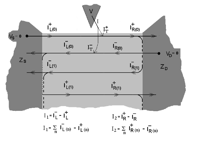
So let us consider the current backscattered from one chiral (plasma) branch to the other: it is NOT the electronic backscattering current which is simply (to the right of the impurity) the difference between the current in the presence of the impurity and the current in the absence of an impurity. This follows from their expression; in a general setting where one has both backscattering and current injection one would have (see Figure 6):
which reduces here to:
by current conservation.
In contrast:
( is the voltage between source and drain). It is a simple matter however to show that in the infinite system . We might say that gives information about the backscattering at the impurity while contains the full backscattering, including the reflections at boundaries.
We turn to the boundary conditions which now include the voltage of source and drain:
Thus :
while:
(by current conservation along the wire).
We define observables and in the absence of the impurity ; they obey
Then for the shifted variables and we get:
The first line simply expresses the fact that the same current is backscattered to the right and to the left of impurity. This is the same set of equations we got with the injected current operators and (see Eq. (32) ) if we identify with . We therefore arrive at the main point of the section, namely that the same matrix equation holds:
It follows that this equation admits the same interpretation as for the STM tip: the current measured in the leads and the current backscattered by the impurity are different objects; we can view the above equation as an operator renormalization of the backscattering current operator, which results from multiple reflections at the boundaries of the system.
IV.2 Finite-frequency.
The previous equations for the tunneling currents at finite frequency
are modified like this:
Observe that at finite frequency that (and that : there is a charging of the system).
IV.3 Reduction of the current correlators to simpler ones.
From the relation between the measured currents and the backscattering current at finite frequency one finds that the currents in a matched geometry obey:
It is therefore convenient to define the following operators since for the matched geometry they will have excpectation values identical to those of the infinite system:
So that at finite frequency:
(and at zero frequency: ).
Finally the relation between the correlators of matched and unmatched system are:
This is the main result of this section: the relation is valid at any temperature, voltage and frequency so long as the LL theory is valid. Note that the renormalization is temperature independent: it comes solely from the physics of impedance mismatch. We stress that this is a non-perturbative relation which must be obeyed by any consistent theory.
IV.4 Excess noise.
We now make the following simplifying assumption, as in the STM problem, namely we approximate the correlators and by their values taken in the infinite system: the rationale for doing this is that again these operators correspond to the impedance matched current operators.
We plug in the expression of the shot noise in the infinite system:
where is the charge of Laughlin excitations and (see chamon ).
Finally:
where and ( and are the lengths from the impurity to each boundary). This is one of the main results of the paper.
Observe that as a subcase of this formula one gets for (and neglecting the small prefactors):
where . This is the expression found using the Keldysh technique by Dolcini et al impurity (the correspondence to the notations of that paper is that our in their notations).
IV.5 Discussion.
Our general formula can be interpreted as follows; it has three main components:
(i) the anomalous charge of the Laughlin excitations;
(ii) a frequency and voltage dependent part which already exists for the infinite LL;
(iii) the third factor is a renormalization.
As a summary this formula is superiour to those existing in the litterature for the following reasons:
(i) it is valid for arbitrary values of the load impedances and at source and drain while other expressions in the litterature stm ; impurity (to the author’s konwledge) are only correct for .
(ii) Other expressions mix two very distinct aspects of the LL parameter : as a characteristic impedance and as a charge of the Laughlin fractional quasiparticles. Indeed they are expressed solely in terms of the parameter : . As a result it may not be conceptually clear whether one measures a fractional charge or just the plain LL parameter . In contrast our expression proves that the noise assumes the simple form (which is a priori unexpected). The formula is actually valid independently of the value taken by the fractional charge: it only relies on the assumption of Poisson scattering of fractional excitations carrying a charge . For Poisson scattering this shows the charge MUST appear as a prefactor and never enters in the renormalizing factor.
For instance if we blur the distinction between , and we might be tempted to argue that since appears as a factor of in the numerator of the expression, measuring the prefactor of this term relative to that of provides a measurement of the inverse square of the anomalous charge : but this is conceptually completely wrong!
(iii) It has been suggested impurity that the integral of the Fano factor over a period yields the charge . However firstly, this is a coincidence for the very special case where and secondly this comes about by neglecting the term : at any rate even if we discard the power-laws in general, the value of that integral is
So it is only by accident that one finds the fractional charge when . It is quite unlikely that one might have both identical electrodes AND an impurity sitting exactly at the middle of the wire (), which is one of the conditions under which the integral has been computed. So the idea that averaging the Fano factor over a period yields the fractional charge is in general incorrect and becomes correct only under some drastic conditions.
If the left and right contact resistances differ, the additional factor enters and can not be discarded. If one uses our more general result for the integral over a period to extract the charge there is still the drawback that one must aim at the range, which is extremely high.
(iv) In contrast and as in the STM geometry since we have expressions depending explictily on the fractional charge we can use them at lower frequencies by measuring deviations to the DC limit, i.e. already in the range of for a 1% variation. The fractional charge will show as a ratio independent of frequency:
(v) Still this remains high. So the method we advocate is again to match impedances at the boundaries of the setup.
V Conclusion and experimental prospects.
We summarize our results.
1. We have computed the DC and AC excess noise of a Luttinger liquid connected to two electrodes using a boundary-conditions formalism describing interface resistances connected to the system. All the expressions for the DC and AC excess shot noise derived in this paper improve on the existing litterature by separating clearly the contributions from the charge of the elementary excitations and the contributions arising from reflections. Both are mixed in other theories because the charges and the reflections both depend on the LL parameter . In contrast our derivations rely on a close analysis of the reflections which enabled us to pinpoint exactly how each factor enters in the shot noise formulas. Additionally our analysis is quite simple and does not need the sophisticated machinery of the Keldysh technique.
2. For the first experimental setup considered (injection of electrons by a STM tip within the bulk of a LL) we found that although (because of reflections at the boundaries) DC shot noise is in general unable to yield information about the fractional charges carried by the elementary excitations of the Luttinger liquid, still by using impedance matching one can recover the fractional charges. For such an impedance matched LL:
| (74) | ||||
| (75) | ||||
| (76) |
which slightly generalizes the expression found in stm by allowing asymetrical injection (to either the right or left Fermi points and ). The predictions of stm for the infinite system should therefore be observable although the system is finite. We note also that our formulas have been established in this paper independently of the exact values of the charges . The LL theory predicts however that: .
If impedance matching is difficult to realize one can still recover the fractional charges through measuring AC shot noise:
where and ( and are the lengths from the impurity to each boundary) and . This should be in the range of , which improves by a factor of ten other experimental proposals which rely on the periodic nature of the noise (as frequency is varied) impurity .
3. Similar conclusions apply to the setup consisting of an impurity sitting in the bulk of a Luttinger liquid. We found that the best method is still to match impedances although fractional charges should show with AC probes as:
Use of our expressions experimentally requires as a prerequisite measurements of three parameters: the characterisitic impedance of the LL and the (boundary) interface resistances and . This can be readily done by AC conductance measurements as explained in p3 .
For matching impedances we observe finally that the tunable impedances need not be at the mesoscopic scale. This actually depends on the measurement one is interested in: our calculations assume interface resistances; usually the length over which there will be relaxation is simply the inelastic scattering length . So if one works at finite frequency , one requires . If the tunable impedances have a size smaller than then they can be considered as being interfacial (as assumed in our calculations) and one need not worry over the spatial extent of the contacting electrode. Therefore for matching impedances at the DC level, the interface impedances can even be macroscopic. Only for higher frequency measurements would one need mesoscopic contacts.
Appendix A On fractionalization.
A.1 Motivation for the ’fractional states picture’ of the Luttinger liquid.
Exact solutions of models which belong to the Luttinger liquid universality class do show fractional excitations. to cite but a few:
- the Heisenberg spin chain has a continuum of spin spinons which are unaccounted for in the low energy mapping of a Luttinger liquid (this would imply charge states in the Fock space of the Jordan-Wigner fermions);
- the Hubbard model has also spinons but additionally shows charge spinless states, the holons.
Yet the description of the Luttinger liquid in the bosonization scheme does not show any fractional states but reveals two kinds of collective excitations are derived:
- plasmons (collective density fluctuations, the bosons of ’bosonization’);
- ’zero-mode’ operators which change the number of fermions by integral increments (the density of left or right moving fermions is changed uniformly: hence the name ’zero-mode’).
(A note on terminology: by fractional states we mean states coming from the fragmentation of the electron and which carry parts of the quantum numbers of the original particle; we do not assume that these parts are rational numbers. They might be irrational numbers.)
The solution of the apparent paradox is simple: the plasmon + zero mode states constitute indeed a complete basis of eigenstates of the LL and there can be no missing states in the diagonalization of the LL. If fractional states exist in the LL they can only form as states in alternate complete bases of eigenstates. This is what we actually proved in fractionalization .
Depending on the physical process under scrutiny a specific eigenbasis may prove more or less convenient. One main drawback of the plasmon + zero-mode basis is that it is not fitted to describe the charge dynamics in terms of elementary processes (involving diffusion of few elementary excitations) because plasmons carry momentum but no charge, while zero-mode excitations have charge but no momentum. Describing the scattering of two fermions by a potential using zero-modes and plasmons would involve an infinite number of plasmon states (this follows from the fact that the fermion operator is an exponential of plasmon operators).
Likewise it is not possible to interpret the shot noise results for a LL with an impurity kane or with a STM tip stm in terms of elementary processes using zero-mode and plasmon states. Fractional states are mandatory. The natural language for transport in a LL is that of fractional states for a LL and this shows up in simpler calculations as this paper shows. So mathematically they are useful tools.
A.2 Fractional ’zero-mode’ operators?
While fractional states appear naturally in a field-theoretical approach of bosonization they translate in the constructive approach ’a la Heidenreich & Haldane’ bosonisation into zero-mode operators with a non-integral power such as:
where is the usual (superfluid) phase conjugate to the number operator :
and with:
which shows that the states are fractional. This can raise consistency problems due to the following technicality: if an operator has integer eigenvalues then it is hermitian only in the space of states periodic for its canonical conjugate field (see especially Appendix D.2 of the second reference in bosonisation ). The above canonical commutation relation for the number operator is therefore somewhat an abuse of language since it would imply on the one hand and on the other, by (erroneously) using the hermiticity of the operator : . So one should apply to periodic functions of the phase field such as and rather use the commutation relation:
This implies that operators such as may lead to similar hermiticity issues.
Actually this difficulty is at the core of the explanation of how fractional states can exist in a system made out of integral charges (electrons) and in spite of the difficulty indeed.
As is clear from the operator has a zero expectation value between states : this is precisely stating that it has a non-integer charge. One might imagine several ways out to ensure such an operator is properly defined: one is to enlarge the Fock space to accomodate states such as but this is of course forbidden. The structure of the Fock space is rigid: it is defined by the electrons. The other way is to create such a fractional state along with another one so that the total charge is an integer: this is what precisely happens in our construction of the fractional bases of states in a LL.
A fractional state is never created in isolation so that one never has inconsistent expectation values; one only meets expressions of the form:
where is an integral number. There is therefore no hermiticity problem. All the expectation values involving these (pairs) of fractional states are perfectly well defined.
The constraint can be viewed as a selection rule on the allowed fractional states. In the case of the LL the two fractional states although created together need only obey such a selection rule and apart from it are completely independent: they will generate continua of excitations parametrized by the two independent dispersions of the two fractional states.
A.3 Description of the fractional states of the LL.
(What follows is merely a heuristic description of the fractional states. For details the reader is referred to Ref. fractionalization ).
The previous picture explaining how fractional states may arise is a little bit more complicated with the actual LL because one then has two species of electrons (left or right moving electrons) and the low-energy Fock space is a direct product of the Fock spaces of each fermion species. This means that one has two kinds of basic number operators and associated canonical conjugate zero-mode fields:
This is not a big complication and one finds additional selection rules. Let us see how.
It is convenient to consider the following zero modes:
where: (the total charge) and: (which is related to the current); obviously: and . The fractional states can be shown to involve operators such as:
Such combinations arise because the diagonalisation of the LL hamiltonian involve similar combinations for the boson fields.
In order to have meaningful expectation values such as:
it is straightforward to show one has to impose the following conditions involving the integers and :
If we invert the relation we have the following constraints on the fractional charges
(The index refers to two counterpropagating chiral modes of the LL.)
Since and are arbitrary (positive or negative) integers the spectrum of the allowed fractional charges forms a two-dimensional lattice.
As for any lattice all the states are spanned by primitive vectors: these vectors represent fractional excitations from which all the others can be built; in other words they are elementary excitations. Here obviously for instance:
But as for any lattice again the choice of a primitive basis is not unique and therefore one will have several equivalent sets of elementary fractional excitations.
As explained above depending on the physical process scrutinized one or another of these basis will be more adapted: in general it will be better to use a basis involving the fewer number of elementary excitations in order to truly describe elementary processes (involving few particles).
The previous basis of states is convenient for processes involving only one of the two species of fermions so that or : it involves two fractional states with charges . These are precisely the states we considered in this paper for the shot noise created by injection of particles by a STM.
Another basis is more convenient when one deals with particle-hole excitations ( so that ):
for , is an even integer and the equation simplifies into:
These excitations with charge are actually the analogs of the Laughlin quasiparticles of the Fractional Qunatum Hall Effect. Indeed for the LL hamiltonian is identical to two counterpropagating copies of the chiral Luttinger liquid edge states at filling ; the operator for the Laughlin quasiparticle of the edge states then coincides exactly with the fractional operator of charge considered here. The main difference is that the charge need not be a rational number.
Another convenient basis involves holon states. If one generalizes these considerations to a spinful LL one finds that such a spinless state is created along with a spin chargeless state, the spinon. One thus recovers the fractional excitations of the Hubbar model. As an aside we mention that the holon state is actually dual to the charge Laughlin quasiparticle (i.e. electromagnetic duality - which exchanges the roles of the electric and magnetic field, or here for the LL, which exchanges current and charge - maps the holon state on the Laughlin quasiparticle). There is therefore a deep connection between the holon of the Hubbard model and the Laughlin quasiparticle of the Fractional Quantum Hall Effect, which should probably come as a surprise.
Finally we mention that for bosons (and spins) different selection rules must be used: although the low-energy field theory (the LL hamiltonian) is the same as that of fermions there are still remnants of the exchange statistics. One finds that:
there are two basic elementary excitations: one is the Laughlin quasiparticle, the other is a charge state which simply corresponds for spin systems to the spinon.
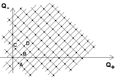
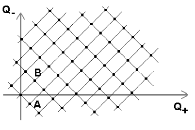
The lattice for fermions is a rectangular centred lattice whose axes are the directions , while for bosons it is a rectangular lattice (with similar axes). These lattices become square lattice for the special values (fermions) or (bosons or spins), which are actually self-dual points in terms of the electromagnetic duality discussed above. For these values the spectrum of elementary excitations involves only one kind of elementary excitation: the free fermion on the one hand, and the spinon on the other hand ( corresponds to the symmetric Heisenberg spin chain).
Appendix B Green’s functions using “impedance boundary conditions”: towards a keldysh treatment.
We define the standard phase field of the LL boson Hamiltonian per:
Using that definition, given the reflection coefficients for the density and at the source and drain boundaries, the reflection coefficients for the phase field are easily shown to be and , namely the chiral components and obey the boundary conditions:
Due to these one can view the propagation as being in a doubled length system (in a loop).
The Green’s function is derived in a standard manner by solving its equation of motion:
The Green’s function can be conveniently divided into four chiral components: where for the causal Green’s functions and appropriate definitions for the retarded Green’s function and so forth. After Fourier transforming one seeks a solution of the following form:
because obey respectively the equations of motion: .
We enforce the ’impedance boundary conditions’ which imply that:
Finally the equations of motion for the chiral Green’s functions are used to extract the undetermined coefficients so that:
where and where the poles are shifted from the real axis according to the usual prescriptions for the causal or retarded Green’s functions, etc. The interpretation of the Green’s function is quite straightforward: to go from one point to the other there are four kinds of basic trajectories, (i) if one is behind the destination going straight to it, or (ii-iii) going after bouncing from one boundary or the other, and (iv) lastly going after bouncing two times from different boundaries. These basic trajectories must then be convoluted by round trips along the whole loop (of length ) which yield the overall factor .
The Green’s function coincides with that of the infinite LL when impedance matching is realized namely: which in turn implies: .
The basic ingredient to use the Keldysh formalism is the Keldysh Green function matrix for that field . The upper time-line is indexed by while the lower time-reversed line is indexed by sign . The following correlator can be extracted from the Green’s function as :
The successive factors correspond to either direct propagation or propagation after reflections at the boundaries. The other matrix elements follow immediately through their definitions and likewise , .
The inhomogeneous LL is found again to be a special case of our general expressions: .
Starting from these one can then use the general relations derived in stm giving the noise spectrum as a function of the Keldysh Green functions: these relations are valid quite generally since resulting from perturbation theory and do not depend on the use of the inhomogeneous LL model.
Appendix C Injected vs measured currents for AC transport.
Let us prove Eq.(62). We must modify the equations defining the currents by specifying the position.
And the boundary conditions:
We can rewrite eveything in terms of fields at the position by taking into account the fact that the fields being chiral:
It is convenient to define the vectors:
Then the boundary conditions can be recast as:
while the definition of the currents imply:
Or in a matrix form:
We solve for and :
The tunneling currents at position and frequency are thus:
Inverting the matrix yields:
where are the currents injected at position (the STM tip). Finally we note that the currents injected at get a phase dependence when reaching the boundaries so that: (this follows simply from the chirality of these currents: implies of course that ). Replacing these expressions we get Eq.(62).
References
- (1) Ya. M. Blanter, M. Büttiker, Phys. Rep. 336, 1 (2000).
- (2) R. de Picciotto et al, Nature (London) 389, 162 (1997); L. Saminadayar, D.C. Glattli, Y. Jin, B. Etienne, Phys. Rev. Lett. 79, 2526 (1997).
- (3) F. D. M. Haldane, J. Phys. C 14, 2585 (1981); H.J. Schulz, in Les Houches Summer School 1994, Mesoscopic Quantum Physics, E. Akkermans et al. eds, Elsevier Science, Amsterdam (1995).
- (4) R. Heidenreich, R. Seiler, A. Uhlenbrock, J. Stat. Phys. 22, 27 (1980); J. von Delft, H. Schoeller, Annalen Phys. 7, 225 (1998).
- (5) K.-V. Pham, M. Gabay, P. Lederer, Phys. Rev. B 61, 16397 (2000).
- (6) C. L. Kane and M. P. A. Fisher, Phys. Rev. Lett. 72, 724 (1994).
- (7) D. Maslov, M. Stone, Phys. Rev. B 52, R5539 (1995); I. Safi, H. Schulz, Phys. Rev. B 52, R17040 (1995); V. V. Ponomarenko, Phys. Rev. B 52, R8666 (1995).
- (8) A. Crépieux, R. Guyon, P. Devillard, T. Martin, Phys. Rev. B. 67, 205408 (2003); A. Lebedev, A. Crépieux, T. Martin, cond-mat/0405325.
- (9) V. V. Ponomarenko and N. Nagaosa, Solid State Commun. 110, 321 (1999).
- (10) B. Trauzettel, F. Dolcini, I. Safi, H. Grabert, Phys. Rev. Lett. 92, 226405 (2004); F. Dolcini, B. Trauzettel, I. Safi, H. Grabert, cond-mat/0409320.
- (11) K-V Pham, Eur. Journ. Phys. B 36, 607 (2003).
- (12) M. W. Bockrath, Ph. D. Thesis, University of California, Berkeley, (1999); P. J .Burke, IEEE Trans. Nanotechn. 1, 129 (2002); IEEE Trans. Nanotechn. 2, 155 (2003).
- (13) K-I Imura, K-V Pham, F. Piéchon, P. Lederer, Phys. Rev. B. 66, 035313 (2002).
- (14) K-V Pham, F. Piéchon, K-I Imura, P. Lederer, Phys. Rev. B. 68, 205110 (2003).
- (15) C. L. Kane and M. P. A. Fisher, Phys. Rev. B. 46, 15233 (1992).
- (16) C. L. Kane and M. P. A. Fisher, in Perspectives in the Quantum Hall Effects, Eds S. Das Sarma, A. Pinczuk (Wiley, New York, 1995).
- (17) R. Egger, H. Grabert, Phys. Rev. B 58, 10761 (1998).
- (18) I. Safi, Ann. Phys. Fr. 22, 463 (1997).
- (19) C. de Chamon, D. E. Freed, X. G. Wen, Phys. Rev. B 53, 4033 (1996).