Interfacial tensions near critical endpoints:
experimental checks of EdGF theory

Abstract

Predictions of the extended de Gennes-Fisher local-functional theory for the universal scaling functions of interfacial tensions near critical endpoints are compared with experimental data. Various observations of the binary mixture isobutyric acid $+$ water are correlated to facilitate an analysis of the experiments of Nagarajan, Webb and Widom who observed the vapor-liquid interfacial tension as a function of both temperature and density. Antonow’s rule is confirmed and, with the aid of previously studied universal amplitude ratios, the crucial analytic “background” contribution to the surface tension near the endpoint is estimated. The residual singular behavior thus uncovered is consistent with the theoretical scaling predictions and confirms the expected lack of symmetry in $(T-T_{c})$. A searching test of theory, however, demands more precise and extensive experiments; furthermore, the analysis highlights, a previously noted but surprising, three-fold discrepancy in the magnitude of the surface tension of isobutyric acid $+$ water relative to other systems.

I Introduction

On passing through a critical endpoint, a binary liquid mixture of, say, species B and C, in the presence of the vapor $\alpha$, exhibits phase separation below $T_{c}$ into two phases $\beta$ and $\gamma$ while above $T_{c}$ there is only one homogeneous liquid phase $\beta\gamma$ Row ; Wid (a, b); NWW . The $\gamma$ phase, rich in C, may be supposed to have the higher density so that in a gravitational field it lies below the $\beta$ phase. In fact there are binary mixtures which display lower consolute points so that phase separation occurs above $T_{c}$ and mixing below $T_{c}$; but since there are found to be no basic differences in criticality, only upper consolute points will be considered explicitly.

Renormalization group theory has recently shown that the critical behavior realized at a critical endpoint lies in the same universality class as on the critical locus that results when the pressure is increased so that the vapor phase $\alpha$ is fully suppressed Die (a, b). Nevertheless, near a critical endpoint, new bulk and interfacial singularities arise Fis (a, b). These are of particular interest in the interfacial tensions $\Sigma_{\beta|\gamma}$, $\Sigma_{\alpha|\beta}$, $\Sigma_{\alpha|\gamma}$, and $\Sigma_{\alpha|\beta\gamma}$ corresponding to the various interfaces indicated by the subscripts Wid (a, b); NWW ; Fis (a, b). Indeed, except for the first, namely $\Sigma_{\beta|\gamma}(T)$, all these tensions are functions both of the temperature, $T$, and of the overall density, $\rho$ (or, equally, of the overall composition).

In terms of the standard notation, with $t\equiv(T-T_{c})/T_{c}$, the behavior of the critical surface tension $\Sigma_{\beta|\gamma}(T)$ that vanishes at the critical endpoint can be described by

$$\Sigma_{\beta|\gamma}(T)\approx K|t|^{\mu},\quad t\to 0-,\quad(h=0),$$ (1)

where $K$ is a nonuniversal critical amplitude while in $d\enspace(\leq 4)$ spatial dimensions the exponent satisfies the scaling relations

$$\mu = 2\beta+\gamma-\nu=2-\alpha-\nu,$$ (2)

$$= \beta(\delta+1)-\nu=(d-1)\nu,$$

first derived, specifically for the surface tension, by Widom Wid (c, d). The symbol $h$ in parentheses in (1) denotes the ordering field [conjugate to the order parameter $\sim\negthinspace(\rho-\rho_{c})$] that is introduced in the scaling description Wid (a, b); Fis (a, b); Zin (a, b). It is an analytic combination of the temperature $T$ and the chemical potentials, $\mu_{B}$ and $\mu_{C}$, or, e.g., the chemical potential difference, $\Delta\mu=\mu_{C}-\mu_{B}$, and the pressure, $p$, (all these being thermodynamic fields in the standard sense); furthermore, $h$ is defined so that it vanishes at the critical endpoint, specified, say, by $(T_{c},\rho_{c},p_{c})$, and is identically zero on the whole $(\beta,\gamma)$ coexistence surface (or phase boundary) in the $(T,\mu_{B},\mu_{C})$ thermodynamic space: see, e.g., Fig. 1 of I Zin (b).

The other surface tensions between the noncritical vapor or spectator phase $\alpha$ and the liquid phases $\beta$, $\gamma$, and $\beta\gamma$ share a common “background” contribution, $\Sigma_{0}(T,h)$, which varies analytically and does not vanish at criticality. Thus we can write Fis (a, b)

$$\Sigma_{\alpha|\beta\gamma}(T) \approx K^{+}|t|^{\mu}+\Sigma_{0}(T,0),\quad t\to 0+,\quad(h=0),$$

$$\Sigma_{\alpha|\beta}(T) \approx K^{-}|t|^{\mu}+\Sigma_{0}(T,0),\quad t\to 0-,\quad(h=0-),$$ (3)

where $K^{+}$ and $K^{-}$ are again nonuniversal amplitudes. When, as generally expected Row , the wetting temperature, $T_{W}$, lies below $T_{c}$, the intermediate $\beta$ phase spreads over the $\alpha|\gamma$ interface; then Antonow’s rule Row ; Zin (b) holds, that is,

$$\Sigma_{\alpha|\gamma}(T)=\Sigma_{\alpha|\beta}(T)+\Sigma_{\beta|\gamma}(T),\quad(h=0)$$ (4)

which by (1) and (3) implies

$$\Sigma_{\alpha|\gamma}(T)\approx(K+K^{-})|t|^{\mu}+\Sigma_{0}(T,0),\quad t\to 0-,\quad h={0+}.$$ (5)

More generally, on the whole thermodynamic surface bounding the $\alpha$ phase, we have

$$\Sigma(T,h)=\Delta\Sigma(T,h)+\Sigma_{0}(T,h),$$ (6)

where $\Delta\Sigma(T,h)$ and $\Sigma_{0}(T,h)$ are the singular and regular (or analytic) parts of the surface tension, respectively. Above $T_{c}$ one has $\Sigma=\Sigma_{\alpha|\beta\gamma}$, while below $T_{c}$ one has $\Sigma=\Sigma_{\alpha|\gamma}$ when, by convention, $h>0$ but $\Sigma=\Sigma_{\alpha|\beta}$ when $h<0$.

According to general scaling principles the singular part can be written asymptotically as

$$\Delta\Sigma(T,h)\approx K|t|^{\mu}S_{M}^{\pm}[\widetilde{m}(T,h)],\quad\quad\quad\quad\widetilde{m}\equiv M(T,h)/B|t|^{\beta},$$ (7)

where the superscripts $+$ and $-$ stand for $t\buildrel>\over{{}_{<}}0$, respectively: see I. Because in experiments the density is more readily accessible than the chemical potentials the argument $\widetilde{m}$ of the scaling functions, $S_{M}^{\pm}(\bullet)$, has been chosen proportional to the order parameter which, in leading order, may be taken as $M\equiv(\rho-\rho_{c})$. The coefficient $B$ represents the coexistence curve amplitude according to $M_{0}\approx B|t|^{\beta}$. The nonuniversal amplitudes $B$ and $K$ are introduced in (7) to make the scaling functions $S_{M}^{\pm}(\bullet)$ and their arguments dimensionless. Then the $S_{M}^{\pm}(\bullet)$ are expected to be universal with, by virtue of Antonow’s rule (4),

$$S_{M}^{-}(1)-S_{M}^{-}(-1)=1.$$ (8)

Owing to the technical and conceptual difficulties arising from the fluctuations of capillary waves, the renormalization group approach has not so far been successful in calculating the $S^{\pm}_{M}(\widetilde{m})$. Instead, advances have been made with the aid of phenomenological theories based on local-functional concepts. The pioneering studies, both theoretical and experimental, have been made by Widom and his co-workers Wid (a, b); NWW . However, as noted in Fis (a, b), their theory predicts a “correction term” varying as $|t|^{\gamma}$ which becomes more singular than the leading $|t|^{\mu}$ term when $d>3-\eta$ as is relevant in real three-dimensional systems. This defect was remedied in the EdGF or “extended de Gennes-Fisher” theory proposed in Fis (a, b) and implemented recently in I Zin (b) which forms the basis for the present report. By using an accurate representation of the equation of state near criticality Zin (a), the EdGF scaling functions $S^{\pm}_{M}(\widetilde{m})$ have been calculated explicitly and presented in I. On evaluating the scaling functions in zero field, one obtains estimates for the Fisher-Upton ratios Fis (a, b), namely,

$$P\equiv(K^{+}+K^{-})/K=0.137_{5}\pm 0.002,\quad Q\equiv K^{+}/K^{-}=-0.834\pm 0.002.$$ (9)

These ratios have been studied experimentally by Woermann and coworkers aKr ; Mai for the binary fluid 2,6-dimethyl pyridine $+$ water: their results are discussed in Sec. II below.

To go further and test the basic theoretical predictions for the interfacial scaling functions $S_{M}^{\pm}(\widetilde{m})$ away from the $h=0$ axis, the notable experimental data of Nagarajan, Webb, and Widom (NWW) NWW for mixtures of isobutyric acid and water offer, to our knowledge, the only available opportunity. For the same mixture, Howland, Wong, and Knobler (HWK) Kno (a) measured the critical surface tension $\Sigma_{\beta|\gamma}(T)$ while Greer Gre (a) measured the densities on the coexistence curve. These two experiments provide what prove to be valuable consistency checks and calibrations for the NWW data as will be seen below.

It may be noted that there are interesting surface-tension experiments on other quasi-binary and binary mixtures, such as $n$-octadecane and $n$-nonadecane in ethane Peg , 2,5-lutidine in water Pri , and 2-butoxyethanol in water Woe . However, our attention will focus on the isobutyric acid $+$ water system since only in this case are there sufficient measurements of the surface tensions near the critical endpoint to warrant an attempt to extract the interfacial scaling functions.

Since the surface tension vanishes at the critical point as $|t|^{\mu}$ with $\mu\simeq 1.26$, and hence faster than linearly, the background contribution to the surface tensions proves highly significant as anticipated in I. Thus, in analyzing the experimental data, it is essential to determine the background $\Sigma_{0}(T,h)$ carefully. By virtue of the analyticity of the background, we may suppose it can be well represented near the critical endpoint, $(t,h)=(0,0)$, by an expansion of the form

$$\Sigma_{0}(T,h)=\Sigma_{c}+\Sigma_{t}t+\Sigma_{h}h+\Sigma_{tt}t^{2}+\Sigma_{th}th+\Sigma_{hh}h^{2}+\cdots.$$ (10)

Examination of the NWW experimental data (see their Fig. 8) reveals a definite upward curvature in the plots of $\Sigma$ vs. $T$ at fixed composition; but the theoretical results for the singular part $\Delta\Sigma(T,0)$ alone shows the opposite, downward curvature above $T_{c}$: see I Fig. 5(a) and the negative value of $Q$ in (9). To capture this dominant behavior, the expansion (10) must contain at least quadratic terms in $t$.

In the analysis reported by NWW of their own data, the background was assumed to be representable by the form

$$\Sigma_{b}(T,M)\simeq\Sigma_{c}+\Sigma_{t}t+\Sigma_{tM}\thinspace tM.$$ (11)

However, this expression is not smooth in $t$ and $h$, as expected on general grounds, since on the critical isotherm it implies $(\partial\Sigma_{b}/\partial t)\simeq\Sigma_{t}+\Sigma_{tM}M$ while $M$ varies as $\hbox{sgn}(h)|h|^{1/\delta}$ with $1/\delta\simeq 0.21$ which is highly singular. Furthermore, the NWW background assumption seems to have led to the conclusion that $S_{M}^{+}(\widetilde{m})$ above $T_{c}$ was indistinguishable from $S_{M}^{-}(\widetilde{m})$ below $T_{c}$: see NWW Fig. 10. However, when a suitable background of the form (10) is used in the analysis, one sees that the data support a difference between $S_{M}^{+}(\widetilde{m})$ and $S_{M}^{-}(\widetilde{m})$ as, indeed, predicted theoretically in I and expected quite generally: see Sec. V below.

Units and Exponents

For convenience of reference we have set out in Table I the exponent values adopted in the analyses reported below. They correspond, of course, to those for the three-dimensional Ising universality class Zin (c); But ; Pel ; Gui ; Cam (a).

Since extensive experimental data will be discussed it is useful to specify here the units employed. Thus: (i) mass densities will be measured in $\hbox{g}/\hbox{cm}^{3}$ and denoted in these units as $\check{\rho}\equiv\rho/(\hbox{g}/\hbox{cm}^{3})$; (ii) for surface tensions, $\Sigma$, and the corresponding amplitudes, $K$, etc., units of erg/cm² will be employed and indicated by $\check{K}$, etc.; (iii) since the reduced free energy density will be taken in $\hbox{cm}^{-3}$ units, appropriate units for the field $h$, conjugate to the order parameter $M=(\rho-\rho_{c})$, are $\hbox{g}^{-1}$ indicated correspondingly by $\check{h}$. The units for various critical amplitudes, $B$, $C^{\pm}$, and the coefficients $\Sigma_{th}$ in (10), etc. follow similarly.

Outline

The balance of this article is set out as follows. In Sec. II, the theoretical predictions (9) for the universal ratios $P$ and $Q$ are discussed in the light of the experiments of Woermann and coworkers aKr ; Mai . The density data of Greer Gre (a) along the coexistence curve of isobutyric acid $+$ water and the corresponding critical surface tension data of HWK Kno (a) are analyzed in Sec. III to determine the critical amplitudes $B$ and $K$. These results are used to calibrate the NWW data which are much more extensive but not as precise and, thus, harder to analyze with confidence on their own. However, the NWW observations are found to be fully consistent with the earlier measurements and, furthermore, confirm the validity of Antonow’s law in the temperature range studied: see Fig. 2 below.

On this basis the analysis can be carried forward to determine the crucial background term, $\Sigma_{0}(t,h)$. The results along the coexistence curve and on the critical isochore above $T_{c}$ (i.e., for zero field, $h\negthinspace=\negthinspace 0$) are reported in Sec. IV.A and displayed in Fig. 3. To estimate $\Sigma_{0}(t,h)$ on the critical isotherm, $T=T_{c}$ $(t=0)$ for nonzero $h$, it is necessary to re-express the NWW observations at constant density in terms of the field. For this purpose one needs information regarding the bulk equation of state that goes beyond the value of $B$. In the absence of direct bulk measurement on the critical isotherm, one can progress by appealing to bulk universal amplitude ratios (known numerically with appreciable reliability Zin (c); But ; Pel ), combined with the further universal critical ratio $S^{+}$ that relates the surface tension amplitude $K$ to the correlation length Zin (c): see (A.1) in the Appendix where the relevant theory is reviewed and its application explained.

By this route one can estimate the amplitude $C^{+}$ for the ordering susceptibility and thence, as explained in Secs. IV.B, IV.C, and the Appendix, the necessary conversions can be implemented. Thereby the field-dependence of the background may be gauged. The singular part, $\Delta\Sigma(t,h)$, then follows by subtraction although, unfortunately, with rather limited precision that precludes, for example, any direct determination of the surface tension amplitudes, $K^{c}_{>}$ and $K^{c}_{<}$, on the critical isotherms. Nevertheless, in Sec. V, the theoretically predicted universal scaling functions are compared in suitable plots with the experimental surface tension data of NWW. To the extent that consistency is well established, the results are encouraging: however, significantly more precise and extensive data close to criticality will be required to enable sharper tests of the theory.

The analysis, furthermore, encounters anew a puzzling dilemma concerning the degree to which the dimensionless surface-tension ratio, $S^{+}$, for the isobutyric acid $+$ water system actually conforms to the expected value in light of independent observations of the critical scattering and the values found for other systems. The issue is brought up in Sec. IV.B and pursued in some detail in the Appendix although without resolution. The considerations presented highlight the need for further experiments and, perhaps, for further theoretical developments.

The article is summarized briefly in Sec. VI.

II Lutidine and Water: Universal Ratios $\bm{P}$ and $\bm{Q}$

Predictions for the surface tension ratios $P$ and $Q$ defined in (9) have been tested experimentally by Mainzer-Althof and Woermann (MW) Mai . A binary liquid mixture of 2,6-dimethyl pyridine [2,6-(CH₃)₂(C₅H₃N)], which is also known as 2,6-lutidine, and water was prepared at the critical composition and used in the experiment. The surface tensions $\Sigma_{\alpha|\beta}(T)$, $\Sigma_{\alpha|\gamma}(T)$, and $\Sigma_{\alpha|\beta\gamma}(T)$ were measured, for the reduced temperature range $-0.028\lesssim t\lesssim 0.019$, by the inverted pendant drop (or rising bubble) method: analysis of the contour line of the bubbles gives the surface tension. Also, the mass densities of the liquid phases $\rho_{\beta}(T)$, $\rho_{\gamma}(T)$, and $\rho_{\beta\gamma}(T)$ were measured. For the critical surface tension, MW re-analyzed the experimental data of Kreuser and Woermann aKr using the new MW density data.

In the MW analysis of the surface tension data, the background (10) was employed truncated at the linear term, $\Sigma_{t}\thinspace t$. At first MW fitted the data to (3) and (5) by allowing separate background terms for $\Sigma_{\alpha|\beta}$, $\Sigma_{\alpha|\gamma}$, and $\Sigma_{\alpha|\beta\gamma}$ (i.e., different sets of $\Sigma_{c}$ and $\Sigma_{t}$) and varying $\Sigma_{c}$, $\Sigma_{t}$, $K^{\pm}$, and $(K+K^{-})$. For the exponent $\mu$ they assumed the value $1.26$. The results did not agree with the original Fisher-Upton (FU) values $P\simeq 0.1_{2}$ and $Q\simeq-0.83$ Fis (a, b). Furthermore, it appeared that Antonow’s rule was not obeyed. However, when the analysis was performed with, as demanded theoretically, a common background, $\Sigma_{0}(T)$, Antonow’s rule was found to be satisfied (as expected): this procedure yielded

$$P_{\rm expt}\simeq 0.00\pm 0.08,\quad Q_{\rm expt}\simeq-1.0\pm 0.2.$$ (12)

The $P$ ratio is evidently not quite consistent with the FU value but, significantly, the $Q$ value is consistent, both in sign and magnitude.

Other fitting procedures were also explored by MW by imposing the theoretical value of either $K^{+}/K\enspace[=PQ/(1+Q)]$ or $K^{-}/K\enspace[=P/(1+Q)]$ and using a common background. Averaging the central values of two different MW fits and extending error estimates to fully cover the fits yield

$$P_{\rm expt}\simeq 0.11^{+0.05}_{-0.08},\quad Q_{\rm expt}\simeq{-0.835}^{+0.06}_{-0.12}.$$ (13)

These values are consistent both with (12) and, now, with the original FU estimates. Furthermore, the more recent improved EdGF estimates for $P$ and $Q$ from I, quoted above in (9), agree remarkably well with these albeit biased fits to the experimental data.

It is appropriate to mention some earlier work. Pegg, Goh, Scott, and Knobler Peg studied quasi-binary mixtures of $n$-octadecane and $n$-nonadecane in ethane and measured the surface tensions through and near both the upper and the lower critical endpoints that occur in the vicinity of the hidden tricritical point that arises in this system. Their data, although limited, certainly support Antonow’s rule and, more importantly for us, suggest strongly that the ratio $K^{+}/K$ is negative and of order unity in accordance with the EdGF predictions. However, the upper and lower endpoints are less than $0.2\thinspace\hbox{\thinspace${}^{\circ}\hbox{\rm C}$}$ apart and, mainly, for that reason, the 8 data points for the surface tensions $\Sigma_{\beta|\gamma}$ (and the 3 for $\Sigma_{\alpha|\gamma}$) are not sufficient to warrant quantitative study.

The surface tension of the water and 2,5-lutidine system has been measured by Privat and co-workers Pri at the critical composition of the lower critical consolute point as well as off that critical composition. The authors claim to verify Antonow’s rule. However, their quoted fits for the amplitudes $K$, $K^{+}$, and $K^{-}$ seem problematical relative to the graphical presentation of their data. Thus, and especially in the light of the MW experiments on the closely related 2,6-lutidine system, this work cannot be regarded as yielding useful experimental estimates for the amplitude ratios $P$ and $Q$.

III Isobutyric Acid and Water: Nonuniversal Amplitudes

III.1 Coexistence Curve Amplitude

The coexistence curve of isobutyric acid $+$ water has been studied carefully by Greer Gre (a), who measured the coexisting mass densities, $\rho_{\beta}(T)$ and $\rho_{\gamma}(T)$, with a precision of 20 ppm from 3.5 K below the critical temperature at intervals as small as 5 mK (with a precision of $\pm 1$ mK) for a sample prepared at close to the critical composition. Two runs were made and the data are recorded in Appendix A of Ref. Gre, a. Greer’s analysis demonstrated that an optimal choice of order parameter (as judged in relation to the number density of a pure fluid in a lattice-gas representation) was the volume fraction of one component, say $\phi_{B}$. The surface tension experiments of NWW, which are of principal concern to us, however, also used the mass density in the vicinity of the critical endpoint as the primary controlled observable. Accordingly, we have reanalyzed Greer’s data using the mass difference, $\rho-\rho_{c}$, as the order parameter. This choice, of course, affects the real (and apparent) magnitudes of the various correction terms; but these will play no more than an auxiliary role in our analysis. Further discussion of fits for the volume fraction difference, $\Delta\phi$, are given in Zin (d): one learns that a range of reasonable fits to the data serve to determine the critical point to within $\pm 10$ to $15$ mK while the leading critical amplitude $B$ can be found with a precision of no better than $\pm 1$ %.

More specifically, we have fitted the data to

$$\hbox{$1\over 2$}\Delta\rho\equiv\hbox{$1\over 2$}\left[\rho_{\gamma}(T)-\rho_{\beta}(T)\right]=B|t|^{\beta}\thinspace[1+b_{\theta}|t|^{\theta}+b_{1}t],$$ (14)

with $t=(T-T_{c})/T_{c}$ as usual, but, as a useful crosscheck, also in terms of the asymptotically equivalent variable,

$$t^{\prime}=1-T_{c}/T=t/(1+t),$$ (15)

as in a previous study Zin (e). Using primes to denote the amplitudes fitted with $t^{\prime}$ we find, from the first run Zin (d),

$$T_{c}\simeq 25.996_{7}\hbox{\thinspace${}^{\circ}\hbox{\rm C}$},\quad\check{B}\simeq\check{B}^{\prime}\simeq 0.03104,$$

$$b_{\theta}\simeq b^{\prime}_{\theta}\simeq-1.73,\quad b_{1}\simeq-9.783,\quad b^{\prime}_{1}\simeq-9.455.$$ (16)

The difference $b^{\prime}_{1}-b_{1}\simeq 0.328$ is close to $\beta$ as it should be for consistency in light of (15).

The exponent $\theta\simeq 0.5$ (See Table I) in (14) specifies the leading correction to scaling. General scaling considerations Fis (c); Kim (a) indicate that a further correction term, $|t|^{2\beta}$, should also be present which, since $2\beta\simeq 0.65<1$, should in fact dominate the linear term. The corresponding amplitude $b_{2\beta}$ may well be rather small: nevertheless, the data cannot resolve two such terms so that the fitted values of the coefficients $b_{\theta}$ and $b^{\prime}_{\theta}$ must be regarded as no more than effective amplitudes.

On setting $b_{\theta}=b_{1}=0$ in (14) Greer found $\check{B}=0.0265\pm 0.0005$; however, on allowing for $b_{\theta}\neq 0$ the value $0.0315\pm 0.0025$ resulted; this is fully consistent with (16). Repeating the same procedure for the second experimental run yields

$$T_{c}\simeq 25.969_{6}\hbox{\thinspace${}^{\circ}\hbox{\rm C}$},\quad\check{B}\simeq\check{B}^{\prime}\simeq 0.03175,$$

$$b_{\theta}\simeq b^{\prime}_{\theta}\simeq-2.635,\quad b_{1}\simeq-14.563,\quad b^{\prime}_{1}\simeq-14.234.$$ (17)

The difference $b^{\prime}_{1}-b_{1}\simeq 0.329$ is again close to $\beta$. Clearly, the deviations of the fitted values here from those in (16) provide a measure of the accuracy available in estimating $T_{c}$ and $B$.

III.2 Comparison with NWW Coexistence Curve Data

We may now use the fits to (14) to calibrate the experiments on the same system by NWW who prepared mixtures of isobutyric acid $+$ water at various compositions and determined the surface tensions by optically measuring the wavelength of surface waves generated by a transducer. In Table 1 of NWW, about 140 $(T,\rho,\Sigma)$ data points are presented: these are what we study here. We have extrapolated some of the observations to the coexistence curve; but, as indicated briefly in Sec. IV.A, only very small changes in the values of $\rho$ and $\Sigma$ are entailed.

To proceed, we first consider the diameter of the coexistence curve in the density variable, namely,

$${\overline{\rho}}(T)=\hbox{$1\over 2$}(\rho_{\beta}+\rho_{\gamma}),$$ (18)

since, as mentioned, the density was directly observed by NWW. Owing to the mixing of thermodynamic fields near criticality in fluids, one expects a dominant singular term $|t|^{1-\alpha}$ to appear in the diameter Fis (c); Kim (a); Wid (e); Reh ; Fis (d). However, the NWW data do not reveal a signature of any such singular term. Rather, the coexistence curve appears almost symmetric in the $(\rho,T)$ plane Gre (b). Thus the diameter may be well represented by a constant as

$${\check{\overline{\rho}}}(T)\simeq\check{\rho}_{c}\simeq 0.9936.$$ (19)

As discussed by Greer Gre (a), the critical temperature of the isobutyric acid $+$ water system is particularly sensitive to ionic impurities Kim (b) and, indeed, experience shows that the observed critical temperatures of nominally the same binary fluid mixtures typically vary from experiment to experiment by amounts exceeding the stated errors. For fitting the NWW data, therefore, we have adopted their value of $T_{c}=26.310\pm 0.001\hbox{\thinspace${}^{\circ}\hbox{\rm C}$}$, even though it lies outside the uncertainty limits implied by (16) and (17). As seen in Fig. 1, by using (14) and (19) with the amplitude estimate

$$\check{B}=0.0314\pm 0.0004,$$ (20)

the NWW data can be represented rather satisfactorily. This demonstrates the consistency of their observations with other careful studies and establishes a reliable estimate for the amplitude $B$ which will be employed below.

It may be remarked that NWW advocated the use in theoretical analysis of a (conventionally defined) volume fraction, $\phi$, in place of the density, $\rho$ Phi . Study of their data reveals, however, that the dependence of $\phi$ on $\rho$ is both surprisingly nonlinear and significantly temperature dependent. Furthermore, contrary to the expectations of NWW (see p. 5781) and Greer, the coexistence curve appears to be more symmetric and regularly behaved in terms of $\rho$ than of $\phi$. Accordingly, we have accepted the directly observed variable $\rho$ as the order parameter in all the following analysis.

III.3 Critical Surface-Tension Amplitude $\bm{K}$

In order to obtain the critical amplitude $K$ as defined for the surface tension in (1), the capillary-rise data obtained by HWK Kno (a) for isobutyric acid $+$ water will be employed. In their Fig. 8, one can clearly see one point that deviates significantly from the general trends, namely, that corresponding in HWK Table VII to $T_{c}-T=1.088$ K or $t\simeq-0.0036$, and $\check{\Sigma}_{\beta|\gamma}=0.0191$. This point has thus been omitted in the present analysis.

Since only eight data points are available, the correction-to-scaling terms are not expected to play a detectable role. First, therefore, the data have been fitted to the form

$$\Sigma_{\beta|\gamma}=\Sigma_{c}+K|t|^{\mu},$$ (21)

where, of course, $\Sigma_{c}\equiv 0$ is anticipated. The reported value of $T_{c}$ is $299\thinspace\hbox{K}$ Kno (a); but we have not found in the account of HWK a satisfying description as to how this value was determined. We therefore adopted

$$T_{c}=299.00\thinspace\hbox{K}=25.85\thinspace\hbox{\thinspace${}^{\circ}\hbox{\rm C}$},$$ (22)

provisionally but have also examined how estimates for $K$ are affected by changes in the assigned value of $T_{c}$.

A weighted least-squares fit then yields

$$\check{\Sigma}_{c}=-0.002\pm 0.008,\quad\check{K}=34.6\pm 5.7,$$ (23)

where the uncertainties quoted here and below are twice the standard deviation. By imposing $\Sigma_{c}=0$, which is clearly consistent with the data, one finds

$$\check{K}=32.8\pm 1.7,$$ (24)

where the central estimate has shifted by 5% while the uncertainty is reduced by 30% in comparison with (23). Repeating the analysis with $\Sigma_{c}=0$ but using $t^{\prime}=t/(1+t)$ as a variable Zin (e), we find $\check{K}=32.6\pm 1.7$ in good agreement.

As a further check one can calculate $\Sigma_{\beta|\gamma}/|t|^{\mu}$ from each data point. This ratio approaches $K$ when $t\to 0$, and an average yields $\check{K}\simeq 32.7$, suggesting that the corrections to the pure power law are relatively small.

To gauge the sensitivity to the imposed value of $T_{c}$, we changed the value by $\pm 0.1$ K. Considering that the temperature was controlled to within $0.01$ K Kno (a), this variation is fairly large. The results (obtained by fixing $\Sigma_{c}=0$) are $\check{K}=30.6\pm 1.7$ for $T_{c}=25.95\thinspace\hbox{\thinspace${}^{\circ}\hbox{\rm C}$}$ and $\check{K}=35.3\pm 1.8$ for $T_{c}=25.75\thinspace\hbox{\thinspace${}^{\circ}\hbox{\rm C}$}$. Despite the changes of $\pm 7$ %, the overlap of the error bars allows consistency with the previous estimates for $K$.

Finally, the data were fitted to $\Sigma=K\thinspace|(T/T_{c})-1|^{\mu}$ treating both $T_{c}$ and $K$ as parameters. Minimizing $\chi^{2}$ yielded $\check{K}\simeq 33.8_{5}$ and $T_{c}\simeq 25.78\thinspace\hbox{\thinspace${}^{\circ}\hbox{\rm C}$}$. This value for $T_{c}$ is $0.07$ K lower than the asserted value (22) but the amplitude estimate again lies in the indicated range. Repeating the procedure with $\Sigma=K^{\prime}\thinspace|1-(T_{c}/T)|^{\mu}$, yields the same value for $T_{c}$ but $\check{K}^{\prime}\simeq 33.5$, about 1% smaller. Overall we believe that

$$\check{K}=33.7\pm 2.5,$$ (25)

summarizes the evidence conservatively Kpr , although a more precise knowledge of $T_{c}$ in the HWK experiments could be valuable.

III.4 Comparison with NWW Critical Surface-Tension Data

It is informative to compare the experiments performed by HWK with those of NWW to check, in particular, for mutual consistency: see Fig. 2. For convenience NWW data points on the coexistence curve have been numbered consecutively from 1 to 15. Except for point 8, other points joined by parallelograms were measured at the same temperature. Points 1–7 lie on the high density side of the coexistence curve and hence represent $\Sigma_{\alpha|\gamma}(T,h\negthinspace=\negthinspace 0+)$, while points 9–15 correspondingly lie on the low density side and represent $\Sigma_{\alpha|\beta}(T,h\negthinspace=\negthinspace 0-)$.

To explain the significance of the fixed-$T$ parallelograms, consider, as an example, points 2 and 14. By Antonow’s rule we have $\Sigma_{\alpha|\gamma}=\Sigma_{\alpha|\beta}+\Sigma_{\beta|\gamma}$ and so by using $\Sigma_{\beta|\gamma}(T)\approx K|t|^{\mu}$ with the estimate (25) and by varying $\Sigma_{\alpha|\beta}$ within the uncertainty limits, one can find a range of $\Sigma_{\alpha|\gamma}$ values that are consistent with Antonow’s rule. Evidently, the central value of the data point 14 corresponds to the lower limit of the data point 2, while the upper limit corresponds to the central value of data point 2. These mutually consistent limiting pairs of the data points 2 and 14 have been joined by parallel lines. In other words, the vertical sides of the parallelogram connecting data points 2 and 14 represent error limits on the NWW data that are consistent with the HWK experiment and with Antonow’s rule. Thus we notice that data point 3 represents a high estimate of $\Sigma_{\alpha|\beta}$ while data point 13 is relatively low. Despite this (3,13) worst case, it can be concluded that the two experiments are mutually consistent and that the estimate $K$ in (25) is reliable Kpr . Note that it would have been very difficult to obtain a reliable value of $K$ from the NWW data alone, owing to the necessity of extrapolating and differencing their (not highly precise) data to obtain $\Sigma_{\beta|\gamma}$ via Antonow’s rule.

III.5 Other Surface Tension Amplitudes

Having determined the two amplitudes $K$ and $B$, which serve as metrical factors in the scaling formulation of the critical-endpoint behavior of the surface tension [see (7)], we are prepared to take the next step towards analyzing the NWW data. The first issue must be to establish the background contribution, $\Sigma_{0}(T,h)$, by estimating the coefficients $\Sigma_{c}$, $\Sigma_{t}$, etc., in (10). To that end it proves helpful to have at hand values for the surface tension amplitudes $K^{+}$ and $K^{-}$ as defined in (3). Ideally, of course, these should be unambiguously determined by the data themselves: but, as already seen in Sec. II, it is unrealistic at this stage in the development of experimental techniques to expect to do more than verify—optimistically at a fully convincing level—consistency of the theory with the observational data. Accordingly, we report here the values

$$\check{K}^{+}=-23.3\pm 1.8,\quad\check{K}^{-}=27.9\pm 2.1,$$ (26)

that follow from (25) on accepting the EdGF calculations for the universal ratios $P$ and $Q$ given in (9).

To determine the field-dependent coefficients $\Sigma_{h}$ and $\Sigma_{hh}$ in the background expansion (10) we will need to examine the data for $\Sigma(t,h)$ on the critical isotherm. The expected behavior is

$$\Sigma_{c}(h)\approx K^{c}_{\buildrel>\over{{}_{<}}}|h|^{\mu/\Delta}+\Sigma_{c}+\Sigma_{h}h+\Sigma_{hh}h^{2},\qquad(T=T_{c})$$ (27)

where, again, values for the amplitudes $\check{K}^{c}_{>}$ and $\check{K}^{c}_{<}$, for $h\buildrel>\over{{}_{<}}0$, respectively, will prove of importance. To estimate these one may appeal to the EdGF theoretical values reported in I (6.9) for the universal ratios

$$S^{c}_{\buildrel>\over{{}_{<}}}\equiv{K^{c}_{\buildrel>\over{{}_{<}}}\over K}\left({B\over C^{+}}\right)^{\mu/\Delta}.$$ (28)

In the second factor in this expression, which enters because $K^{c}_{\buildrel>\over{{}_{<}}}$ and $K$ have different dimensions, the nonuniversal amplitude $C^{+}$ specifies the magnitude above $T_{c}$ of the divergence of the basic ordering susceptibility as $1/t^{\gamma}$. Note that the notation for amplitudes used here and below accords with that set out in the Appendix of Zin (c).

The appropriate value of $C^{+}$, and of other nonuniversal amplitudes for isobutyric acid $+$ water, is taken up in Sec. IV.B when the field-dependence is considered explicitly. At that stage, we will make contact with Moldover’s extensive analysis Mol (a, b) of surface tension, light scattering, and bulk thermodynamic experiments for a range of single-component and binary fluid systems designed to test the hyperscaling (or “two-scale factor universality”) hypothesis for criticality. Various details and some questions they raise are presented in the Appendix.

IV Determination of the Surface Tension Background

As discussed in Sec. I, to analyze the NWW surface tension measurements appropriately, the background $\Sigma_{0}(T,h)$ must at least contain quadratic terms in $t$; it then seems reasonable to include quadratic terms in $h$ also as in (10). In order to determine the background coefficients $\Sigma_{c}$, $\Sigma_{t}$, etc., we adopt the following strategy. First, the data on the $h\negthinspace=\negthinspace 0$ axis, i.e., for the mixture at the critical composition, will be fitted to obtain $\Sigma_{c}$, $\Sigma_{t}$, and $\Sigma_{tt}$. From the data on the critical isotherm, $t=0$, the coefficients $\Sigma_{h}$ and $\Sigma_{hh}$ can then be examined. Finally, to obtain the cross-term coefficient $\Sigma_{th}$, the derivative $(\partial\Sigma/\partial t)_{h}$ may be studied on the critical isotherm.

IV.1 Along the Coexistence Curve

In zero-field, the surface tension above $T_{c}$ is, following the Introduction, expected to behave as

$$\Sigma_{\alpha|\beta\gamma}(T)\approx K^{+}|t|^{\mu}+\Sigma_{c}+\Sigma_{t}t+\Sigma_{tt}t^{2},\qquad(T\geq T_{c}).$$ (29)

Below $T_{c}$, there are two distinct vapor-liquid interfaces and two surface tensions, $\Sigma_{\alpha|\beta}$ and $\Sigma_{\alpha|\gamma}$, corresponding to the coexisting phases $\beta$ and $\gamma$. By Antonow’s rule (which as shown is satisfied by the NWW data) the difference $(\Sigma_{\alpha|\gamma}-\Sigma_{\alpha|\beta})$ is the critical surface tension $\Sigma_{\beta|\gamma}$ and thus it suffices to study only $\Sigma_{\alpha|\beta}(T)$ below $T_{c}$. The identical expression (29) then applies except that $K^{+}$ is to be replaced by $K^{-}$.

To proceed, one may first fit $\Sigma_{\alpha|\beta\gamma}(T)$ using the data above $T_{c}$ at the very close-to-critical composition tabulated by NWW, by regarding $K^{+}$, $\Sigma_{c}$, $\Sigma_{t}$, and $\Sigma_{tt}$ as free parameters. These fits suggest $K^{+}>0$ which, in accord with the generally observed upwards curvature (compare with I Fig. 5), has the opposite sign to the prediction for $K^{+}$ in (26). We conclude that the NWW data above $T_{c}$ are not, on their own, of adequate precision to reliably distinguish the amplitudes of three terms varying as $t$, $t^{\mu}$, and $t^{2}$; hence, we cannot independently estimate $K^{+}$.

However, as indicated in the MW analysis Mai discussed in Sec. II, the situation may be improved by imposing the theoretical value of the ratio $K^{+}/K$; but this is then equivalent to imposing $K^{+}$ because, as seen in Sec. III, the critical amplitude $K$ has been already estimated reliably by comparison with the HWK data. Since $\Sigma_{\alpha|\beta\gamma}(T)$ and $\Sigma_{\alpha|\beta}(T)$ share the common background $\Sigma_{0}(T,0)$, we likewise impose $K^{-}$ as given in (26). Of course, by adopting this procedure we will be primarily checking the consistency of our theory with the NWW data which, unfortunately, are not adequate for estimating $K^{+}$ and $K^{-}$ directly as might originally have been hoped.

Accordingly, by subtracting the singular term in (29) and likewise below $T_{c}$, we can generate experimental data for the zero-field background alone: see Fig. 3. Again we use the NWW data taken at the (close-to) critical composition above $T_{c}$ and the (close-to) low-density side of the coexistence curve. A least-squares fit then yields

$$\check{\Sigma}_{c}\simeq 26.284,\quad\check{\Sigma}_{t}\simeq-14.6,\quad\check{\Sigma}_{tt}\simeq 381.$$ (30)

The corresponding plot is represented by the dashed curve in Fig. 3 and seen to be very good. This demonstrates that these coefficient estimates are most reasonable although, as will be discussed, they prove to be less than fully satisfactory in the near critical region below $T_{c}$.

To examine the fit further consider the plots shown in Fig. 2. The dashed curve represents the surface tensions $\Sigma_{\alpha|\beta}(T)$ and $\Sigma_{\alpha|\gamma}(T)$ on the coexistence curve as reproduced from the amplitudes $K$ and $K^{-}$ and the background coefficients (30): to translate $t\propto T_{c}-T$ into the density on the coexistence curve, the inner fit described in the caption of Fig. 1 is used. The agreement with the central values of the NWW data on the low-density side is encouraging; however, the fit reveals significant, systematic discrepancies on the high density side where the plot lies outside the observational range for all the points 1–7.

To complement the overall or “full-range” approach just described and to understand the discrepancies uncovered on the high-density side of the coexistence curve, let us return to Fig. 2 and focus on the data closest to criticality. In particular, as explained in the construction of the parallelograms in this figure, consistency with the HWK data for $\Sigma_{\beta|\gamma}(T)$, together with Antonow’s rule Fen requires that the allowed observational uncertainties quoted for the NWW data should be reduced to correspond to the vertical sides of each parallelogram. Accordingly, for $T\lesssim T_{c}$ consider the truncated forms

$$\Sigma_{\alpha|\beta}(T) \simeq K^{-}|t|^{\mu}+\Sigma_{c}+\Sigma_{t}t,$$ (31)

$$\Sigma_{\alpha|\gamma}(T) \simeq (K^{-}+K)|t|^{\mu}+\Sigma_{c}+\Sigma_{t}t,$$ (32)

in which the background has been restricted to a linear term. By trial and error, one can discover those values of $\Sigma_{c}$ and $\Sigma_{t}$ that give acceptable fits to those data points lying closest to the critical point, specifically, for the pairs (7,9), (6,10), (5,11), (4,12), and (3,13). Slight shifts in the nominal value of $\rho_{c}$ from (19) may also be examined but are found to be detrimental for changes exceeding $\Delta\check{\rho}_{c}=10^{-4}$.

The predominant conclusion is that $\Sigma_{c}$, the common value of the surface tensions $\Sigma_{\alpha|\beta}$, $\Sigma_{\alpha|\gamma}$, and $\Sigma_{\alpha|\beta\gamma}$ at criticality, cannot actually be as low as suggested by the full-range fit (30). The acceptable “critical fits” yield, instead, the range

$$\check{\Sigma}_{c}=26.294\pm 0.004.$$ (33)

Indeed, NWW actually quote the estimate $\check{\Sigma}_{c}\simeq 26.30$, which is much closer to this “critical value” than to (30). The corresponding preferred value for the background slope, is found to be $\check{\Sigma}_{t}=-17.5$; but reasonable fits could be obtained in the range $-16.5>\check{\Sigma}_{t}>-18.5$. In all these fits, however, the fitting curve in Fig. 2 became too broad at the larger values of $|\rho-\rho_{c}|$, failing to fit the data-point pairs (1,15) and (2,14). This last defect, however, was overcome by including in (31) and (32) the quadratic term $\Sigma_{tt}t^{2}$. As the assigned value $\Sigma_{tt}$ is increased, keeping $\Sigma_{c}$ fixed as proves essential, the optimal value for $\Sigma_{t}$ correspondingly falls. Thus $\check{\Sigma}_{t}=-16.0$ and $\check{\Sigma}_{tt}=250$ give very good fits in Fig. 2. However, these particular values do not describe well the highest data points above $T_{c}$ in Fig. 3 (for $t>0.015$). One could well disregard this range since the data extend below $T_{c}$ only down to $|t|\simeq 0.011$. However, one can find values that prove rather satisfactory in fitting all the $h=0$ data, i.e., on the coexistence curve and at the critical composition above $T_{c}$, namely,

$$\check{\Sigma}_{c}\simeq 26.294,\quad\check{\Sigma}_{t}\simeq-15.0,\quad\check{\Sigma}_{tt}\simeq 400.$$ (34)

These coefficients yield the solid curve shown in Fig. 3: evidently the fit displays a systematic displacement above the central values of the data points but by rather small amounts that remain within all the uncertainty ranges. Furthermore, the agreement with the coexistence data is now much improved as seen by the solid curve in Fig. 2. Only very minor departures from the acceptable uncertainty ranges now arise. Accordingly we will retain the assignment (34) in all the following analysis.

At this stage we may conclude that the NWW data are, first, fully consistent with the best previous observations of the coexistence curve and the critical surface tension and, second, are quite consistent with the EdGF based estimates of the ratios $K^{+}/K$ and $K^{-}/K$ even though, unfortunately, the data cannot critically test these ratios.

IV.2 On the Critical Isotherm

It transpires, in retrospect, that NWW did not make observations of the surface tensions very close to the critical isotherm $T=T_{c}=26.310\thinspace\hbox{\thinspace${}^{\circ}\hbox{\rm C}$}$. We may, however, presume that the isotherms just above and below $T_{c}$, namely, at $T=26.49\thinspace\hbox{\thinspace${}^{\circ}\hbox{\rm C}$}$ and $T=26.05\thinspace\hbox{\thinspace${}^{\circ}\hbox{\rm C}$}$ constitute rough lower and upper bounds, respectively, on $\Sigma_{c}(h)$. On the critical isotherm, the surface tension should behave as in (27) with $\mu/\Delta\simeq 0.806$. The optimal assignment of the critical point value $\Sigma_{c}$ has already been determined in the previous subsection. One might wish to determine the amplitudes $K^{c}_{>}$ and $K^{c}_{<}$ directly from the data; but, regrettably there is, once again, no hope of that! Rather, with the limited aim of testing only consistency with the theory, we will adopt theoretical estimates for these two amplitudes. At this point one encounters a rather sharp and surprising dilemma: as explained further in the Appendix, two significantly different sets of EdGF-based predictions arise from (28) and I (6.9). The first set, derives entirely from the two metrical factors $K$ and $B$, that we have determined for isobutyric acid $+$ water, combined with well-confirmed values for various universal critical amplitude ratios Zin (c): as explained in the Appendix this yields

$$\hbox to0.0pt{\hskip 0.0pt\hbox{{\bf A}:}\hss}\check{K}^{c}_{>}=(5.0\pm 0.6)\negthinspace\times\negthinspace 10^{-18},\quad\quad\quad\check{K}^{c}_{<}=-(1.5_{5}\pm 0.1_{7})\negthinspace\times\negthinspace 10^{-18}.$$ (35)

The second set also utilizes the estimate (25) for $K$ in (28) together with (20) for $B$; but instead of using the purely theoretically derived value, namely,

$$\hbox to0.0pt{\hskip 0.0pt\hbox{{\bf A}:}\hss}\check{C}^{+}=(3.04\pm 0.30)\negthinspace\times\negthinspace 10^{-26},$$ (36)

for the amplitude $C^{+}$ in (28), it employs the much larger estimate

$$\hbox to0.0pt{\hskip 0.0pt\hbox{{\bf B}:}\hss}\check{C}^{+}=(14.2\pm 0.6)\negthinspace\times\negthinspace 10^{-26},$$ (37)

that follows, as explained in the Appendix, from independent light scattering and thermodynamic experimental data for isobutyric acid $+$ water Mol (a, b). This then leads to the alternative estimates

$$\hbox to0.0pt{\hskip 0.0pt\hbox{{\bf B}:}\hss}\check{K}^{c}_{>}=(17.5\pm 1.5)\negthinspace\times\negthinspace 10^{-18},\quad\quad\quad\check{K}^{c}_{<}=-(5.4\pm 0.5)\negthinspace\times\negthinspace 10^{-18},$$ (38)

that, likewise, are much larger than in (35).

Granted the values of $K^{c}_{\buildrel>\over{{}_{<}}}$ in the critical point background (27), one is left with only the coefficients $\Sigma_{h}$ and $\Sigma_{hh}$ to be determined by fitting. However, since the NWW measurements were made in terms of the density, it is necessary to convert the $(t,M\negthinspace=\negthinspace\rho\negthinspace-\negthinspace\rho_{c})$ data to $(t,h)$ using an equation of state. To this end, it is natural to employ the scaled equation of state derived in Zin (a) on the basis of the extended sine model. The metric factor $B$ given in (20) and the appropriate values of $C^{+}$ [in (36) or (37)] may be used. The data spread over the range $-4.8\times 10^{21}\lesssim\check{h}\lesssim 2.4\times 10^{20}$ [using (36)] and, hence, reach more widely on the negative $h$ (or low density) side; but for fitting we will focus on the available symmetric range.

On the basis of the A values above we thus find that the assignment

$$\check{\Sigma}_{h}\simeq 3.72\negthinspace\times\negthinspace 10^{-23}\quad\quad\quad\hbox{and}\quad\quad\quad\check{\Sigma}_{hh}\simeq 6.65\negthinspace\times\negthinspace 10^{-43},$$ (39)

provides a fit that lies well between the upper and lower limits for $|h|$ not too large: see Fig. 4. Comparable fits can be found using the B values but with, of course, substantially different values of $\Sigma_{h}$ and $\Sigma_{hh}$ and a different accessible range of $h$. For the balance of this article, however, we will stay with the ‘purely theoretical’ A estimates (35) and (36).

IV.3 Cross Term

In order to estimate the cross coefficient $\Sigma_{th}$ in the background (10), one should examine the derivative $(\partial\Sigma/\partial t)_{h}$ at $T=T_{c}$. Since the measurements were made at constant $M$ (or density), it is appropriate to invoke the relation

$$\left(\frac{\partial\Sigma}{\partial t}\right)_{\negthinspace\negthinspace h}=\left(\frac{\partial\Sigma}{\partial t}\right)_{\negthinspace\negthinspace M}+\left(\frac{\partial\Sigma}{\partial M}\right)_{\negthinspace\negthinspace t}\left(\frac{\partial M}{\partial h}\right)_{\negthinspace\negthinspace t}.$$ (40)

However, owing to the measurement uncertainties, the estimates of $(\partial\Sigma/\partial t)_{M}$ obtainable from the NWW data are extremely noisy. Hence, one cannot seriously attempt to estimate $\Sigma_{th}$. One may reasonably guess, nevertheless, that the geometric mean of $\Sigma_{tt}$ and $\Sigma_{hh}$, namely, using (34) and (39),

$$\left(\check{\Sigma}_{tt}\check{\Sigma}_{hh}\right)^{1/2}=1.6\negthinspace\times\negthinspace 10^{-20},$$ (41)

will provide some indication of the possible order of magnitude of the cross-coefficient. However, we comment below on the sensitivity of the final comparisons with experiment to the value of $\Sigma_{th}$.

V Scaling Functions for the Surface Tension

Having found, to the somewhat limited degree feasible, a reasonable description of the important surface-tension background, we may examine the experimental data for consistency with the predicted universal scaling functions $S_{M}^{\pm}(\widetilde{m})$ introduced in (7).

In order to subtract the background $\Sigma_{0}(t,h)$, from the full surface tension data, it is necessary, as before, to convert the variables $(t,M\negthinspace=\negthinspace\rho\negthinspace-\negthinspace\rho_{c})$ to $(t,h)$ because the experiments employed the density as a primary variable. Adopting the NWW critical temperature $T_{c}=26.310\thinspace\hbox{\thinspace${}^{\circ}\hbox{\rm C}$}$ and using $B$ from (20), the first step is to compute $\widetilde{m}=\penalty-100000(\rho-\rho_{c})/B|t|^{\beta}$. The universal, scaled equation of state $\widetilde{m}=Q_{\pm}(\tilde{h})$ [for $t\buildrel>\over{{}_{<}}0$] may be used in the form of the extended sine model of Zin (a) to implement the conversion to $\tilde{h}$. The corresponding $h$ follows via $h=B\tilde{h}|t|^{\Delta}/C^{+}$ where, for the present discussion we use (36) for $C^{+}$ as in Fig. 4. Then, using the background with the coefficients given in (34) and (39), an estimate for the singular part of the surface tension, $\Delta\Sigma(T,h)$, can be extracted from the NWW data.

Note that in the first instance, the cross term, $\Sigma_{th}th$, may simply be dropped. The resulting scaling contribution, $\Delta\Sigma/K|t|^{\mu}$, is plotted versus $\widetilde{m}$, the scaled density deviation, in Fig. 5.

Since the field-dependence of the background $\Sigma_{0}(t,h)$ has been estimated only from data that lie on the two isotherms closest to criticality and fall within the restricted range $|\check{h}|\lesssim 2.4\negthinspace\times\negthinspace 10^{20}$, we have distinguished, by solid dots versus crosses and plusses, between these observations, corresponding to the restricted range of $h$, and (selected) further data falling outside this range.

Because the background contribution constitutes such a large part of the total surface tension, it is not surprising that the subtraction needed to isolate the singular piece, $\Delta\Sigma(t,h)$, is subject to relatively large uncertainties. This appears to be the main reason why many of the crosses and plusses, derived from the low-density data (beyond the fitted range of $h$), fall significantly below the scaling loci. For the data inside the range (the solid dots in Fig. 4), the agreement between the theoretical and experimental results is moderately encouraging considering the uncertainties of the original data and the inherent difficulties of the analysis. Certainly, the data of NWW support the expected difference between $S_{M}^{+}(\widetilde{m})$ and $S_{M}^{-}(\widetilde{m})$.

It may be noted, nevertheless, that just as pointed out by NWW, the logarithmic singularity associated with the complete-wetting transition cannot be detected in these or other surface-tension plots. However, this is due not only to the limited precision of the experimental data but also to the fact that in the usual representations of the data the singularity is not really visible even in theoretical plots where it is known analytically to be present: compare with Figs. 5 and 6 of I.

If one also includes a positive cross-coefficient $\Sigma_{th}$ in the background with the magnitude given in (41), one finds slight changes of less than 1% in the data points plotted in Fig. 5. However, when the cross-term is inserted with a negative sign, the majority of the data points display changes of $\sim\negthinspace 5$% and a few points prove still more sensitive. This situation is hardly satisfying but, in light of the experimental challenges and the resulting precision of the NWW data, it is clear that our analysis can proceed little further.

Finally, as pointed out theoretically by Ramos-Gómez and Widom Wid (b) and mentioned briefly in I, the surface tension isotherms when examined vs density ($\propto M$) above $T_{c}$ should, in general, exhibit crossings. Although hints of such crossings have appeared in some binary fluid systems Cam (b); McL ; Las , they were not seen in the NWW experiments. The primary reason seems to be that for the range of densities $\rho>\rho_{c}$ explored, the isotherms chosen for observation above $T_{c}$ were somewhat too widely spaced. Indeed, as illustrated in Fig. 6, the anticipated crossings for isobutyric acid $+$ water can be exhibited on the basis of our fits to the NWW data. All that is needed is to choose temperatures above $T_{c}$ spaced apart by intervals of no more than $1\thinspace\hbox{\thinspace${}^{\circ}\hbox{\rm C}$}$ and to extend the observations to densities slightly further above $\rho_{c}$. The crossings, while sensitive to the presence of the background term, should be visible even in the singular part of the surface tension, $\Delta\Sigma(T,\rho)$. Note, however, that since our fits were based only on the restricted (symmetric) range of $h$, the plots lying above the short horizontal lines in Fig. 6 may be less reliable than at lower densities.

VI Summary

In pioneering experiments to study critical endpoint behavior, Nagarajan, Webb, and Widom NWW made extensive measurements of the vapor-liquid interfacial tension of isobutyric acid and water mixtures as a function of temperature at various compositions. Since the precision of the surface tension data was somewhat limited, we used the observations of the critical surface tension made by Howland et al. Kno (a) and the coexistence curve measurements of Greer Gre (a) to cross-calibrate the NWW data. We found full consistency between the various observations and verified agreement with Antonow’s rule near the critical endpoint. In this way reliable estimates of the coexistence curve amplitude $B$ and the surface tension amplitude $K$ were obtained: see (20) and (25). Using known universal amplitude ratios Zin (c) and these two amplitudes, which can serve as the only required metric factors in a hyperscaling formulation, we estimated the nonuniversal susceptibility amplitude $C^{+}$. Thereby the experimental data as a function of density could be transformed in order to uncover the field-dependence of the crucial surface-tension background contribution in the form (1.10). Owing to the considerable uncertainties, however, we could not resolve the cross-coefficient $\Sigma_{th}$. Nevertheless, even without this term, the scaling plots for the singular part of the interfacial tension as derived from the experimental data proved consistent with the theoretical predictions based on the EdGF theory of I Zin (b): see Fig. 5.

On the other hand, as discussed in the Appendix, significant discrepancies come to light when the Howland et al. data are compared, via hyperscaling expectations, with evidence from other critical systems. Owing to conflicting experimental reports Kpr ; Mol (a), however, it seems impossible to resolve this issue and assess its significance without further experiments and, perhaps, new theoretical insights.

More rewarding from a theoretical perspective and less open to questions of precision, the critical surface tension measurements of Mainzer-Althof and Woermann Mai on 2,6-dimethyl pyridine $+$ water at the critical composition, show rather satisfactory agreement between the experimentally determined universal ratios $P$ and $Q$ [see (1.9)] and the EdGF predictions. However, as regards the full scaling aspects of the theory, more detailed, more precise and more reliable data are sorely needed to execute more searching tests!

*

Appendix A Nonuniversal Critical Amplitudes

In Sec. III the coexistence curve amplitude $B$ for isobutyric acid $+$ water (IBA:W) was determined from the data of Greer Gre (a) and checked against the NWW data yielding (20). Likewise, analysis of the HWK capillary-rise surface tension data yielded the critical amplitude $K$ reported in (25) that also accords well with the NWW data using forced capillary waves: indeed, no larger deviation in (25), than, say, $\pm 6.0$ (or $\pm 18$%) could be reconciled with the NWW observations Tha . We stress this point because Moldover Mol (a), in comparing these IBA:W data with results for many other fluid systems, uncovered an inconsistency in the value of the expected-to-be universal amplitude ratio

$$S^{+}\equiv\bar{K}(\xi^{+}_{1})^{2}=0.377\pm 0.011\quad\quad\quad\hbox{with}\quad\quad\quad\bar{K}\equiv K/k_{B}T_{c}.$$ (42)

Here, in the notation of the Appendix and Table I of Zin (c), the amplitude $\xi^{+}_{1}$ specifies the magnitude of the divergence of the second-moment correlation length above $T_{c}$ via $\xi_{1}(T)\approx\xi^{+}_{1}/t^{\nu}$, while the value quoted for $S^{+}$ is that reported in Zin (c).

If we now accept this theoretical result we may proceed to predict the value of $\xi_{1}^{+}$ for IBA:W. Thence, using the universal ratio Zin (c)

$$S_{0}\equiv C^{+}\bar{K}/B^{2}\xi^{+}_{1}=1.17\pm 0.06,$$ (43)

together with the estimates for $K$ and $B$, we can compute the susceptibility amplitude $C^{+}$ that is needed in Sec. V to establish the $h$ scale in Fig. 4. This route, indeed, yields the A value for $C^{+}$ reported in (36) and, with the further aid of (28) and I (6.9), the values for $K^{c}_{>}$ and $K^{c}_{<}$ given in (35). These results, in turn, are incorporated in the plots in Fig. 5 that serve to test the scaling hypothesis.

The correlation length amplitude predicted in this fashion is $\xi_{\rm 1,pre}^{+}=2.10\pm 0.08\thinspace\thinspace{\buildrel\kern 1.49994pt\scriptstyle\circ\over{A}}$ [where the HWK value (22) has been adopted for $T_{c}$ in (42)]. However, as reported by Moldover Mol (a), in light scattering experiments by Chu and co-workers Chu (a, b), the second-moment correlation length above $T_{c}$ was evaluated for IBA:W. The fits presented led them to conclude $\nu\simeq 0.613$ and $\xi_{1}^{+}=3.57\pm 0.07\thinspace\thinspace{\buildrel\kern 1.49994pt\scriptstyle\circ\over{A}}$. This correlation amplitude exceeds the predicted value, $\xi^{+}_{1,{\rm pre}}$, by 60% or more! On re-analyzing their data with the higher value $\nu=0.632$ imposed, we obtain $\xi_{1}^{+}=3.09\pm 0.05\thinspace{\buildrel\kern 1.49994pt\scriptstyle\circ\over{A}}$. This is somewhat closer to $\xi_{1,\rm pre}^{+}$ although the uncertainty limits fail to overlap by 36%. From turbidity measurements, Beysens et al. Bey concluded $\xi_{1}^{+}=3.62_{5}\pm 0.06_{5}\thinspace{\buildrel\kern 1.49994pt\scriptstyle\circ\over{A}}$ and $\nu\simeq 0.630$; this value of $\xi_{1}^{+}$ agrees with Chu et al. and is some 17% higher than that from our reanalysis.

At a basic theoretical level the discrepancies uncovered here are of serious concern. If, for concreteness, one accepts $\xi^{+}_{\rm 1,expt}\simeq 3.6_{0}\pm 0.07\thinspace\thinspace{\buildrel\kern 1.49994pt\scriptstyle\circ\over{A}}$ as the observed value, in accord with these experiments, the universal ratio $S^{+}$ in (42) would yield a prediction for $\check{K}$ of only 12.0, about 36% of that observed! Conversely, one might be tempted to assert that the experimentally determined value of the (supposedly universal) ratio for IBA:W is $S^{+}_{\rm expt}=1.06\pm 0.03$, in place of (42), the uncertainty indicated here taking into account various sources of experimental and theoretical imprecision.

Similarly, the B values for $C^{+}$ and $K^{c}_{\buildrel>\over{{}_{<}}}$ reported in (37) and (38) follow from the observed value of $B$ and the experimental value, $\xi_{1,\rm expt}^{+}$, by using Zin (c)

$$Q_{c}\equiv(\xi_{1}^{+})^{3}B^{2}/C^{+}=0.323_{6}\pm 0.006.$$ (44)

In facing this discrepant situation let us focus first on the theoretical value (42) for $S^{+}$ (which, indeed, was incorporated into the numerical scaling calculations reported in I and tested here). One might initially notice that 0.377 is significantly higher than the various theoretical, RG and Monte Carlo estimates, namely, $\simeq\negthinspace 0.21$, $0.24$, and $0.28$, available to Moldover in 1985 Mol (a). In fact (42) rests on the analysis Zin (e) of difficult but carefully performed Monte Carlo simulations for the nearest-neighbor $(d=3)$-dimensional Ising model by Hasenbush and Pinn Pin (combined with the well established universal ratio $\xi_{1}^{+}/\xi_{1}^{-}=1.96\pm 0.01$ Zin (e); Liu ). The simulations Pin could approach criticality no closer than $|t|>0.015$. By contrast, the experimental data for IBA:W lie in the region $|t|=0.0008$ to $0.010$. Although it seems unlikely, it is conceivable that exceptionally strong correction-to-scaling terms in the surface tension of the simple cubic Ising model could dominate very close to $T_{c}$ so that (42) represents a significant under-estimate of $S^{+}$. Alternatively, finite-size effects in the simulations may be playing a far larger role than appreciated although no evidence to suggest this was observed and the issue was by no means neglected Gel ; Pin .

On the other hand, it might be that for reasons associated with the lattice structure and capillary-wave fluctuations, the standard simple cubic lattice gas/Ising model is inadequate for certain real fluid mixtures. Most certainly, the conventional near-neighbor lattice gases neglect the long-range power-law van der Waals interactions that lead to interphase potentials decaying, normal to an interface, only as $1/z^{3}$. And while these van der Waals forces play only a subdominant role in bulk critical behavior, they are known to be especially significant in surface and wetting phenomena Die (c). It is, thus, possible that they seriously distort the near critical interfacial tension or even destroy the expected universal character of the ratio $S^{+}$.

At present, however, effective theoretical tools for addressing this interesting issue are not apparent. Furthermore, it is not unfair to remark that these various rather deep theoretical issues do not directly affect our basic scaling analysis of the NWW observations of surface tensions near a critical endpoint. Indeed, in the first instance only the experimentally determined critical amplitudes $K$ and $B$ enter: universal or nonuniversal relations between these and other critical amplitude do not play a definitive role in the primary scaling issues.

Finally, we must return to the experimental evidence. It is, indeed, striking that the value for $S^{+}$ in (42) accords remarkably well with the experimental values assembled by Moldover Mol (a) for Ar, Xe, ${\rm N}_{2}$, ${\rm O}_{2}$, ${\rm CO}_{2}$, ${\rm CH}_{4}$ and ${\rm SF}_{6}$ and for the binary fluids triethylamine $+$ water, nitroethane $+$ 3-methylpentane, cyclohexane $+$ aniline, methanol $+$ cyclohexane, and even for various polystyrene $+$ ${\rm C}_{7}{\rm H}_{14}$ solutions: see Fig. 1, Table I and also the Note added regarding Ref. 86 in Mol (a) and Table I of Mol (b). Indeed, by and large, Moldover’s analysis confirms rather generally the hyperscaling hypothesis, both for the interfacial and for the bulk thermodynamic properties. (See also in Zin (d).)

These observations tend to reinforce confidence in the estimate (42) for the universal surface tension amplitude—at least as regards ‘simple’ pure fluids and binary mixtures. But does the weak acid IBA:W constitute such a ‘simple’ system? On the one hand, as an electrolyte, a population of positive and negative ions will be present in all the liquid phases. Furthermore, it is known that the critical point of IBA:W is extremely sensitive to small impurities and, especially, to ionic impurities Gre (a); Kno (b). Ionic impurities, in particular, may be expected to have significant effects on the various liquid-liquid, liquid-vapor and liquid-solid interfaces; but even in the absence of impurities, an interphase Galvani potential difference will appear across the critical liquid-liquid interface together with an associated electrically charged double layer REF (a, b, c, d).

On the other hand, Moldover Mol (a) in addressing the discrepancy issue notes, as a private communication from I. L. Pegg and C. M. Knobler, that further surface-tension measurements on IBA:W using a different technique (actually light scattering from thermally excited capillary waves Kno (b)) yielded the preliminary result $\check{K}=11.6\pm 1.0$. This value is almost three times smaller than found in the HWK experiments with which, as indicated above, it cannot be reconciled. Nevertheless, if this value for $\check{K}$ is used with the experimentally determined values, $\xi_{1,\rm expt}^{+}$, discussed above it yields a value for $S^{+}\propto\check{K}(\xi_{1}^{+})^{2}$ close to that found experimentally for the other systems and, hence, in accord with the expected universal value stated in (A.1) Mol (a, b)! On this basis one might (despite Tha ) be tempted to disregard the HWK data and argue that our analysis of the NWW observations should be seriously reconsidered.

Unfortunately, the preliminary study of IBA:W by Pegg and Knobler has never been published Kno (b); nor, to our knowledge, have any subsequent measurements been made by others on this system. Thus, while one can and, perhaps, should attribute the nearly three-fold difference in the critical surface tension to unidentified impurities or other agencies distinguishing the HWK and NWW samples of isobutyric acid from the later sample investigated by Pegg and Knobler (in 1984), the true causes of the discrepancies and their significance remain obscure. We must, instead, hope that more sensitive techniques will be developed and employed on the IBA:W and other binary systems in order to more stringently test the scaling theories for critical endpoints that have been developed.

 

Table 1: Adopted values of fluid critical exponents. For convenience and consistency with the universal amplitude ratios assembled in Zin (c) we have employed the corresponding exponent values (satisfying the scaling relations). More recent studies But ; Pel ; Gui ; Cam (a) lead to our currently preferred exponent estimates shown here in parentheses. However, for the present analysis the differences are of negligible consequence. We may supplement the relations (2) with $\Delta=\beta\delta=\beta+\gamma$ and $\gamma=(2-\eta)\nu$.

$\beta$	$\gamma$	$\nu$	$\mu$	$\theta$
0.3266	1.2392	0.6308	1.2616	0.54
(0.3260)	(1.2390)	(0.6303)	(1.2606)	(0.52)

FIGURE CAPTIONS

FIG. 1. The coexistence curve of the isobutyric acid and water mixture. The dots represent the experimental data of NWW. The inner curve is the fit (14) using the amplitude $\check{B}=0.0310$ with $a_{\theta}$ and $a_{1}$ from (16) while the outer curve employs $\check{B}=0.0318$ in accord with (17); the critical temperature has been taken as $T_{c}=26.310\hbox{\thinspace${}^{\circ}\hbox{\rm C}$}$ in accord with the estimate of NWW.

FIG. 2. Comparison of surface-tension measurements along the coexistence curve: the open circles with error bars represent the NWW data. As explained in the text, the parallelograms have been drawn using $\Sigma_{\beta|\gamma}=K|t|^{\mu}$ with the amplitude (25) obtained from the HWK data. The vertical sides of the parallelograms indicate the ranges in which consistency between the two experiments can be achieved in accord with Antonow’s rule. The dashed curve, is based on the fit (30) obtained below for the background $\Sigma_{0}(T,0)$, while the solid curve embodies the values (34). See text in Sec. IV.A for details.

FIG. 3. The fit to the surface tension background in zero-field. See text for details of the generation of the data points (black dots). The dashed curve is drawn using the estimates (30). The solid curve represents the fit (34).

FIG. 4. A fit for the surface tension on the critical isotherm as a function of the ordering field. The dots joined by the dashed lines represent the NWW isotherms nearest the critical temperature that serve as approximate upper and lower bounds. See text for details.

FIG. 5. Comparison of scaling plots for the vapor-liquid surface tension near the critical endpoint of isobutyric acid $+$ water. The solid curves represent the theoretically predicted scaling functions $S_{M}^{\pm}(\widetilde{m})$ using the ameliorated EdGF theory. The dots are derived from the NWW data for $T>T_{c}$ and $T<T_{c}$ that fall within the symmetric range $|\check{h}|\lesssim 2.4\negthinspace\times\negthinspace 10^{20}$ used in fitting the surface tension background. The other symbols ($\times$ for $T>T_{c}$ and $+$ for $T<T_{c}$) are some of the NWW data falling outside the symmetric range of $h$ (and hence not covered by the background fit). Note that an offset of $\Delta S=100$ has been used for clarity in the vertical scales for $T\buildrel>\over{{}_{<}}T_{c}$. See the text for further details.

FIG. 6. Illustration of predicted crossings of surface-tension isotherms of isobutyric acid $+$ water above $T_{c}$. The isotherms have been computed using the EdGF scaling functions $S^{\pm}_{M}(\widetilde{m})$ from I with a background of the form (10) suitably matched to the experimental data. The dotted, solid, dashed, and dot-dashed curves represent isotherms $\Delta T\equiv T-T_{c}=0$, $1.0$, $2.0$, and $3.0\hbox{\thinspace${}^{\circ}\hbox{\rm C}$}$, respectively. The narrow horizontal and vertical lines mark the critical values of $\Sigma$ and $\rho$. The short horizontal lines mark the ordering field values up to which the fitting was performed. See the text for further details.

Figure 1:

Figure 2:

Figure 3:

Figure 4:

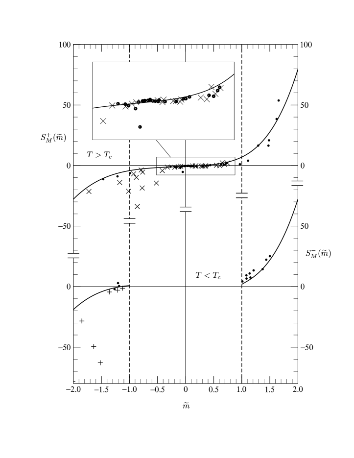
Figure 5:

Figure 6:

References

- (1) J.S. Rowlinson, B. Widom, Molecular Theory of Capillarity, Oxford University Press (1982), chap. 9.
- Wid (a) B. Widom, J. Chem. Phys. 67, 872 (1977).
- Wid (b) F. Ramos-Gómez, B. Widom, Physica A 104, 595 (1980).
- (4) N. Nagarajan, W.W. Webb, B. Widom, J. Chem. Phys. 77, 5771 (1982), to be denoted here as NWW.
- Die (a) H.W. Diehl, M. Smock, Physica A 281, 268 (2000).
- Die (b) H.W. Diehl, M. Smock, Eur. Phys. J. B 21, 567 (2001).
- Fis (a) M.E. Fisher, P.J. Upton, Phys. Rev. Lett. 65, 2402 (1990).
- Fis (b) M.E. Fisher, P.J. Upton, Phys. Rev. Lett. 65, 3405 (1990).
- Wid (c) B. Widom, J. Chem. Phys. 43, 3892, 3898 (1965).
- Wid (d) B. Widom, in Phase Transitions and Critical Phenomena, C. Domb, M.S. Green (Ed.), Academic, London (1972), vol. 2, p. 79.
- Zin (a) M.E. Fisher, S.-Y. Zinn, P.J. Upton, Phys. Rev. B 59, 14533 (1999); ibid. 64, 149901 (E) (2001).
- Zin (b) S.-Y. Zinn, M.E. Fisher, Phys. Rev. E 71, 011601 (2005) [cond:mat/0410673] to be denoted I.
- (13) H. Kreuser, D. Woermann, J. Chem. Phys. 97, 7757 (1992).
- (14) T. Mainzer-Althof, D. Woermann, Physica A 234, 623 (1997).
- Kno (a) R.G. Howland, N.-C. Wong, C.M. Knobler, J. Chem. Phys. 73, 522 (1980) to be denoted HWK.
- Gre (a) S.C. Greer, Phys. Rev. A 14, 1770 (1976).
- (17) I.L. Pegg, M.C. Goh, R.L. Scott, C.M. Knobler, Phys. Rev. Lett. 55, 2320 (1985).
- (18) M. Amara, M. Privat, R. Bennes, E. Tronel-Peyroz, Europhys. Lett. 16, 153 (1991).
- (19) J. Ataiyan, D. Woermann, Pure Appl. Chem. 67, 889 (1995).
- Zin (c) M.E. Fisher, S.-Y. Zinn, J. Phys. A 31, L629 (1998).
- (21) P. Butera, M. Comi, Phys. Rev. B 62, 14837 (2000).
- (22) A. Pelissetto, E. Vicari, Phys. Repts. 368, 549 (2002).
- (23) R. Guida, J. Zinn-Justin, J. Phys. A 31, 8103 (1998).
- Cam (a) M. Campostrini, A. Pelissetto, P. Rossi, E. Vicari, Phys. Rev. E 65, 066127 (2002).
- Zin (d) S.-Y. Zinn, Ph.D. thesis, University of Maryland, 1997, chap. 5. Note that the value was adopted here for some of the analysis: that corresponds to the value that Greer Gre (a) reports as a good fit to the volume fraction difference on neglecting any correction terms to the leading power law. However, within the overall accuracy obtainable, this deviation from the value in Table I has no serious consequences here.
- Zin (e) S.-Y. Zinn, M.E. Fisher, Physica A 226, 168 (1996).
- Fis (c) M.E. Fisher, G. Orkoulas, Phys. Rev. Lett. 85, 696 (2000).
- Kim (a) Y.C. Kim, M.E. Fisher, G. Orkoulas, Phys. Rev. E 67, 061506 (2003): see especially Eq. (3.20) and prior material.
- Wid (e) B. Widom, J.S. Rowlinson, J. Chem. Phys. 52, 1670 (1970).
- (30) N.D. Mermin, J.J. Rehr, Phys. Rev. Lett. 26, 1155 (1971).
- Fis (d) M.E. Fisher, Phys. Rev. Lett. 34, 1634 (1975).
- Gre (b) In contrast to the NWW data, the coexistence curve measured by Greer Gre (a) is somewhat less symmetric: on the basis of her data, the diameter can be represented by .
- Kim (b) See also Y.C. Kim, M.E. Fisher, J. Phys. Chem. 105, 11785 (2001).
- (34) NWW supposed the volume fraction of water in the mixture to be related to the mass fraction via where is a constant that represents the ratio of the density of pure isobutyric acid to that of pure water at . (B. Widom, private communication.).
- (35) Moldover in his review of experiments on many systems Mol (a), quotes from HWK; but as we discuss further in the Appendix, Moldover also reports the value on the basis of a private communication from I. L. Pegg and C. M. Knobler: unfortunately, these two values are drastically inconsistent. However, since the first accords well with our analysis of both the HWK and NWW data, we proceed, at this point, with the estimate (3.12).
- Mol (a) M.R. Moldover, Phys. Rev. A 31, 1022 (1985).
- Mol (b) H. Chaar, M.R. Moldover, J.W. Schmidt, J. Chem. Phys. 85, 418 (1986). It should be noted that in summarizing the data on other binary systems in Table I the authors accept, without discussion, the “preliminary result” of Pegg and Knobler for the critical surface tension amplitude of isobutyric acid water as cited in Ref. Mol (a). See further the discussion in the Appendix here.
- (38) W. Fenzl, Europhys. Lett. 24, 557 (1993) has discussed the NWW data and challenged the validity of Antonow’s rule for their experiments. However, as pointed out in the article by Fenzl himself (B. Widom, private communication), the direction in which it is argued that the rule is violated actually contradicts thermodynamic interfacial stability. In Fig. 2 the tendency for the high-density surface tension data to rise up (relative to the parallelogram) and vice-versa for the low-density data, indicates a trend (violating stability) that Fenzl may have noticed. Otherwise, Fenzl also argues that, contrary to our approach and the theoretical analysis of NWW, the critical behavior they observed corresponds to a very small surface field (and, correspondingly, small ). In light of the observations just made concerning Antonow’s rule and the successful fits we achieve here, Fenzl’s proposal does not seem sustainable.
- Cam (b) A.N. Campbell, E.M. Kartzmark, S.C. Anand, Y. Cheng, H.P. Dzikowski, S.M. Skrynk, Can. J. Chem. 46, 2399 (1968).
- (40) I.A. McLure, B. Edwards, J. Chem. Phys. 70, 3999 (1979).
- (41) We are indebted to B. Widom for drawing our attention to Refs. Cam (b) and McL .
- (42) This point has been reconfirmed by C. M. Knobler who has kindly re-examined the original records of the HWK experiments and sees no reasonable sources of larger errors.
- Chu (a) B. Chu, S.P. Lee, W. Tscharnuter, Phys. Rev. A 7, 353 (1973).
- Chu (b) B. Chu, F.J. Schoenes, W.P. Kao, J. Am. Chem. Soc. 90, 3042 (1968).
- (45) D. Beysens, A. Bourgou, P. Calmettes, Phys. Rev. A 26, 3589 (1982).
- (46) M. Hasenbusch, K. Pinn, Physica A 203, 189 (1994); see also M. Hasenbusch, Int. J. Mod. Phys. C 12, 911 (2001).
- (47) A.J. Liu, M.E. Fisher, Physica A 156, 35 (1989).
- (48) M.P. Gelfand, M.E. Fisher, Physica A 166, 1 (1990).
- Die (c) See, e.g., S. Dietrich in Phase Transitions and Critical Phenomena, C. Domb, J.L. Lebowitz (Ed.), vol. 14, p. 1.
- Kno (b) Private communications from C. M. Knobler and I. L. Pegg. The records of the Pegg–Knobler observations have been generously made available to us: we have confirmed that they differ by more than a factor of two from the HWK and NWW measurements.
- REF (a) See J.-N. Aqua, S. Banerjee, M.E. Fisher, arXiv cond-mat/0410692 (2004) and REF (b, c, d).
- REF (b) M.J. Sparnaay, The Electrical Double Layer, Pergamon Press, Oxford (1972), pp. 4, 338.
- REF (c) J.O’M. Bockris, A.K.N. Reddy, Modern Electrochemistry, Plenum Press, New York (1970), vol. 2, sec. 7.2.5.
- REF (d) P.B. Warren, J. Chem. Phys. 112, 4683 (2000).