Abstract

Within this paper we outline a method able to generate truly minimal basis sets which describe either a group of bands, a band, or even just the occupied part of a band accurately. These basis sets are the so-called NMTOs, Muffin Tin Orbitals of order N. For an isolated set of bands, symmetrical orthonormalization of the NMTOs yields a set of Wannier functions which are atom-centered and localized by construction. They are not necessarily maximally localized, but may be transformed into those Wannier functions. For bands which overlap others, Wannier-like functions can be generated. It is shown that NMTOs give a chemical understanding of an extended system. In particular, orbitals for the $\pi$ and $\sigma$ bands in an insulator, boron nitride, and a semi-metal, graphite, will be considered. In addition, we illustrate that it is possible to obtain Wannier-like functions for only the occupied states in a metallic system by generating NMTOs for cesium. Finally, we visualize the pressure-induced $s\rightarrow d$ transition.


Keywords: Wannier functions, density functional calculations, electronic structure, muffin-tin orbitals, solid-state

1 Introduction

The electronic structure of condensed matter is usually described in terms of one-electron basis sets. Basis functions used for computation are often simple, e.g. Gaussians or plane waves, but their number is large, 1-2 orders of magnitude larger than the number of electrons to be described. This is so because the potential in the effective one-electron Schrödinger equation, arising say in density-functional theory, is rather deep inside the atoms. The results of this kind of computation therefore require interpretation and simplification in terms of a small set of intelligible orbitals. The results of band-structure calculations for crystals, for instance, are often parametrized in terms of tight-binding models.

The Car-Parinello technique for performing ab initio molecular-dynamics simulations using density-functional theory, pseudopotentials, plane-wave basis sets, and supercells, [1] created a need to visualize chemical bonds, and this caused renewed interest in generating localized Wannier functions for the occupied bands. For a set of $M$ isolated energy bands, $\varepsilon_{j}\left(\mathbf{k}\right),$ the Wannier functions, $w_{m}\left(\mathbf{r-T}\right),$ enumerated by $m$ $\left(=1,..,M\right)$ and by the $N$ $\left(\rightarrow\infty\right)$ lattice translations, $\mathbf{T,}$ is a set of orthonormal functions which spans the eigenfunctions,

$$\Psi_{j\mathbf{k}}\left(\mathbf{r}\right)=N^{-\frac{1}{2}}\sum_{\mathbf{T}}\sum_{m=1}^{M}w_{m}\left(\mathbf{r-T}\right)u_{jm}\exp i\mathbf{k\cdot T}$$ (1)

with eigenvalues $\varepsilon_{j}\left(\mathbf{k}\right),$ of the one-electron Schrödinger equation. The Bloch states (1) are delocalized, and the set is enumerated by the band index $j$ and the Bloch vector $\mathbf{k.}$ Wannier functions are not unique, because performing a unitary transformation, $W_{m,m^{\prime};\mathbf{T-T}^{\prime}},$ of one set produces another set which also satisfies Eq. (1), merely with different $j\mathbf{k}$-dependent phases of the Bloch functions. For molecules, it had long been recognized that chemical bonds should be associated with those linear combinations of the occupied molecular orbitals which are most localized, because those linear combinations are most invariant to the surroundings. [2] For infinite periodic systems, Mazari and Vanderbilt have developed a useful method for projecting from the Bloch states a set of so-called maximally localized Wannier functions. [3, 4, 5]

This paper deals with a different kind of basis set, specifically, minimal basis sets of localized orbitals, the newly developed NMTOs (Muffin Tin Orbitals of order N, also known as $3^{rd}$ generation MTOs. [6, 7, 8, 9]) We shall demonstrate that with NMTOs it is possible to generate Wannier functions directly, instead of via projection from the delocalized Bloch states. NMTOs are constructed from the partial-wave solutions of Schrödingers equation for spherical potential wells (overlapping muffin tins) and NMTO sets are therefore selective in energy. As a consequence, one can construct an NMTO set which picks a specific set of isolated energy bands. Since NMTOs are atom-centered and localized by construction, they do –after symmetrical orthonormalization– form a set of localized Wannier functions which, if needed, can be recombined locally to have maximal localization. The NMTO technique is primarily for generating a localized, minimal basis set with specific orbital characters, and it can therefore be used also to pick a set of bands which overlap other bands outside the energy region of interest. The corresponding NMTOs –orthonormalized or not– we refer to as Wannier-like.

NMTO-generated Wannier functions have so-far been used only in a few cases to visualize chemical bonding [9, 10] and more often to construct Hubbard Hamiltonians for strongly correlated 3$d$-electron systems. [11, 12, 13, 10] In the future, it may be possible to use NMTOs for real-space electronic-structure methods in which the computational efford increases merely linearly with system size, so-called order-$N$ methods. [14, 15]

In this paper we will focus mainly on showing how NMTOs may be used to pick specific states in insulating, semi-metallic and metallic systems, namely boron, graphite, and cesium. Since NMTOs are unfamiliar to most readers of this issue, and more complicated than plane waves, we start out by illustrating the main ideas by performing an elementary analytical calculation of the $\pi$-bonds in the simplest tight-binding (TB) model of benzene. Then follows a concise summary of the NMTO formalism.

2 NMTO basics

2.1 Tight-binding calculation of the benzene $\pi$-bond

The simplest TB model for the six $\pi$-electrons in benzene has six orthonormal $p_{z}$-orbitals, $\varphi_{1},...,\varphi_{6},$ placed on the consecutive corners of the hexagon. The hopping integrals over the short (double) bonds are: $H_{12}=H_{34}=H_{56}=-\left(1+d\right),$ and those over the long (single) bonds are: $H_{61}=H_{23}=H_{45}=-\left(1-d\right)$, where $d$ is the dimerization.

In order to calculate the Wannier function for the three occupied bonding states, it is convenient to partition the orbitals into those on the even $\left(e\right)$- and those on the odd $\left(o\right)$-numbered sites. The eigenvalue equations are then: $H_{oo}u_{o}+H_{oe}u_{e}=\varepsilon 1_{oo}u_{o}$ and $H_{eo}u_{o}+H_{ee}u_{e}=\varepsilon 1_{ee}u_{e},$ in terms of the 3$\times 3$ blocks of the Hamiltonian and the unit matrices. Solving the last set of equations for the eigenvector for the even orbitals yields:

$$u_{e}=\left(\varepsilon-H_{ee}\right)^{-1}H_{eo}u_{o},$$ (2)

and inserting in the first equations results in the eigenvalue equation:

$$\left[H_{oo}+H_{oe}\left(\varepsilon 1_{ee}-H_{ee}\right)^{-1}H_{eo}\right]u_{o}=\varepsilon 1_{oo}u_{o},$$ (3)

for the (Löwdin) downfolded Hamiltonian.

In the present case where there is no hopping between even or odd sites, $H_{ee}=H_{oo}=0.$ Moreover,

$$H_{eo}=H_{oe}^{\dagger}=\left(\begin{array}[]{ccc}-\left(1+d\right)&-\left(1-d\right)&0\\ 0&-\left(1+d\right)&-\left(1-d\right)\\ -\left(1-d\right)&0&-\left(1+d\right)\end{array}\right),$$

and

$$H_{oo}+H_{oe}\left(\varepsilon 1_{ee}-H_{ee}\right)^{-1}H_{eo}=\frac{1}{\varepsilon}\left(\begin{array}[]{ccc}2\left(1+d^{2}\right)&1-d^{2}&1-d^{2}\\ 1-d^{2}&2\left(1+d^{2}\right)&1-d^{2}\\ 1-d^{2}&1-d^{2}&2\left(1+d^{2}\right)\end{array}\right).$$ (4)

The latter, downfolded Hamiltonian is periodic with period $3$ and is therefore diagonalized by the unitary transformation

$$U_{ok}=\left(\begin{array}[]{ccc}\frac{1}{\sqrt{3}}&\frac{-1}{\sqrt{2}}&\frac{-1}{\sqrt{6}}\\ \frac{1}{\sqrt{3}}&\frac{1}{\sqrt{2}}&\frac{-1}{\sqrt{6}}\\ \frac{1}{\sqrt{3}}&0&\frac{2}{\sqrt{6}}\end{array}\right),$$ (5)

yielding singly degenerate $a$-states $\left(k=0\right)$ with $\varepsilon=\pm 2$ and doubly degenerate $e$-states $\left(k=\pm 1\right)$ with $\varepsilon=\pm\sqrt{1+3d^{2}}.$ The even components of the eigenvectors are obtained from equation (2): $U_{ek}=\varepsilon^{-1}H_{eo}U_{ok},$ and finally we can renormalize: $u=U/\sqrt{2}.$

Having found all six Bloch eigenstates, we need to form three Wannier functions, that is, three congruent linear combinations of the bonding states. The three downfolded $p_{z}$-orbitals, $\chi_{o},$ defined by: $\chi_{o}U_{ok}=\varphi_{o}u_{ok}+\varphi_{e}u_{ek},$ are obviously congruent. Moreover, they are localized in the sense that $\chi_{1}$ vanishes on the other odd sites ($3$ and 5). In the present case, they are also orthonormal and, hence, Wannier functions. Left-multiplication with $\left(U_{ok}\right)^{-1}=U_{ko}$ yields:

$$\chi_{1}=\frac{1}{\sqrt{2}}\left[\varphi_{1}+\left(\frac{2}{3}+d\right)\varphi_{2}+\left(\frac{2}{3}-d\right)\varphi_{6}-\frac{1}{3}\varphi_{4}\right],$$ (6)

and $\chi_{3}$ and $\chi_{5}$ by cyclic permutation of site indices. Here and in the following, we work merely to first order in the dimerization, $d.$ The Wannier function in Eq. (6) is essentially the NMTO. It is atom-centered and, as the dimerization increases, it becomes lopsided towards site $2,$ i.e., it spills into the short bond. It breaks the symmetry (when $d\neq 0)$ because it was chosen to vanish on the odd sites different from its own, and it is not maximally localized (unless $d=0)$. Nevertheless, it is a fairly simple matter to achieve maximal localization and, hence, to restore the symmetry, by finding a unitary transformation, $W_{T-T^{\prime}},$ which maximizes e.g. $\left\langle\left|w\right|^{4}\right\rangle\equiv\sum_{R=1}^{6}\left|w\right|^{4}.$ Here, $w_{1}\equiv\sum_{T}W_{1-T}\chi_{T}$ is the maximally localized Wannier function. In the present case, $W$ has only one independent matrix element and we find:

$$w_{1}=\frac{1}{3\sqrt{2}}\Bigg{\{}\left(\sqrt{3}+1+\frac{\sqrt{3}}{2}d\right)\left(\varphi_{1}+\varphi_{2}\right)+\left(1-\sqrt{3}d\right)\left(\varphi_{3}+\varphi_{6}\right)$$

$$-\left(\sqrt{3}-1-\frac{\sqrt{3}}{2}d\right)\left(\varphi_{4}+\varphi_{5}\right)\Bigg{\}},$$ (7)

which is clearly symmetric (bond-centered). From (6): $\left\langle\left|\chi\right|^{4}\right\rangle=\frac{19}{54}+O\left(d^{2}\right),$ and from (7): $\left\langle\left|w\right|^{4}\right\rangle=\frac{19}{54}+\frac{2\sqrt{3}}{9}d+O\left(d^{3}\right).$ Hence, for $d=0,$ the atom-centered and the bond-centered Wannier functions are both maximally localized and symmetric.

Now, the NMTO set, $\chi_{o}^{\left(N\right)},$ is obtained without solving the eigenvalue equations, i.e., is not obtained by projection from the Bloch states through multiplication by $\left(U_{ko}\right)^{-1},$ but in a more tricky way: We first define a set of downfolded, energy-dependent orbitals,

$$\phi_{o}\left(\varepsilon\right)\equiv\varphi_{o}1_{oo}+\varphi_{e}\left(\varepsilon 1_{ee}-H_{ee}\right)^{-1}H_{eo},$$ (8)

which are localized when $\varepsilon$ does not coincide with an eigenvalue of $H_{ee}.$ Projection onto the even sites yields: $\left\langle\varphi_{e}\left|\hat{H}-\varepsilon\right|\phi_{o}\left(\varepsilon\right)\right\rangle=0_{oo},$ so we realize that the functions of the set $\phi_{o}\left(\varepsilon\right)$ are solutions of the impurity problems specified by the boundary conditions that $\phi_{o}\left(\varepsilon\right)$ vanishes at the other odd sites and is normalized to $\varphi$ at its own site. Projection onto the odd sites yields:

$$\left\langle\varphi_{o}\left|\hat{H}-\varepsilon\right|\phi_{o}\left(\varepsilon\right)\right\rangle=H_{oo}+H_{oe}\left(\varepsilon 1_{ee}-H_{ee}\right)^{-1}H_{eo}-\varepsilon 1_{oo}\equiv-G_{oo}\left(\varepsilon\right)^{-1},$$ (9)

and comparison with (3) shows that, if $\varepsilon$ is an eigenvalue of the (downfolded) Hamiltonian and $u_{o}$ an eigenvector, then $\phi_{o}\left(\varepsilon\right)u_{o}$ is an eigenfunction. $G\left(\varepsilon\right)$ defined in (9) is the resolvent. Finally, we need to find an energy-independent, $N$th-order approximation to the set $\phi_{o}\left(\varepsilon\right)$: We form the set, $\phi_{o}\left(\varepsilon\right)G_{oo}\left(\varepsilon\right),$ of (contracted Greens) functions and add an analytical function of energy determined in such a way that the two sets of functions, $\phi_{o}\left(\varepsilon\right)G_{oo}\left(\varepsilon\right)$ and $\chi_{o}^{\left(N\right)}G_{oo}\left(\varepsilon\right),$ coincide when $\varepsilon$ is on an energy mesh, $\epsilon_{0},...\epsilon_{N},$ specifying the energy range of interest. By taking the highest-order finite difference on this mesh, one obtains:

$$\chi_{o}^{\left(N\right)}\frac{\Delta^{N}G_{oo}}{\Delta\left[0...N\right]}=\frac{\Delta^{N}\phi_{o}G_{oo}}{\Delta\left[0...N\right]},$$ (10)

which determines the set of (non-orthonormal) NMTOs. For $N=1,$ for instance:

$$\chi_{o}^{\left(1\right)}=\left[\phi_{o}\left(\epsilon_{1}\right)G_{oo}\left(\epsilon_{1}\right)-\phi_{o}\left(\epsilon_{0}\right)G_{oo}\left(\epsilon_{0}\right)\right]\left[G_{oo}\left(\epsilon_{1}\right)-G_{oo}\left(\epsilon_{0}\right)\right]^{-1}.$$ (11)

For the simple benzene model, Eq. (8) yields:

$$\phi_{1}\left(\varepsilon\right)=\varphi_{1}-\frac{1+d}{\varepsilon}\varphi_{2}-\frac{1-d}{\varepsilon}\varphi_{6},$$

and $\phi_{3}\left(\varepsilon\right)$ and $\phi_{5}\left(\varepsilon\right)$ by cyclic permutation of site indices. To order $d,$ the downfolded Hamiltonian (4) is independent of $d,$ and by subtracting $\varepsilon$ and inverting, we find:

$$G_{oo}\left(\varepsilon\right)=\frac{\varepsilon}{\left(\varepsilon^{2}-1\right)\left(\varepsilon^{2}-4\right)}\left(\begin{array}[]{ccc}\varepsilon^{2}-3&1&1\\ 1&\varepsilon^{2}-3&1\\ 1&1&\varepsilon^{2}-3\end{array}\right).$$

Specializing to $N=1,$ the LMTO found from (11) is:

$$\chi_{1}^{\left(1\right)}=\varphi_{1}-\frac{\epsilon_{0}+\epsilon_{1}}{\left(\epsilon_{0}\epsilon_{1}+4\right)\left(\epsilon_{0}\epsilon_{1}+1\right)}\{\left[\epsilon_{0}\epsilon_{1}+2+\left(\epsilon_{0}\epsilon_{1}+4\right)d\right]\varphi_{2}+$$

$$\left[\epsilon_{0}\epsilon_{1}+2-\left(\epsilon_{0}\epsilon_{1}+4\right)d\right]\varphi_{6}-2\varphi_{4}\},$$

and if, with the benefit of hindsight, we choose $\epsilon_{0}=-2$ and $\epsilon_{1}=-1,$ we obtain the exact result (6), apart from the normalization, 1/$\sqrt{2}$. With other choices, the LMTO set is an approximation to the exact Hilbert space spanned by $\chi_{o}$ or $w_{o},$ as explained in connection with Eq. (2.2) below. We leave it to the reader to convince himself that had we chosen $\epsilon_{0}=2$ and $\epsilon_{1}=1,$ we would have obtained the Wannier functions for the antibonding levels.

By considering a simple TB model, we have thus learned that the NMTO procedure for constructing a minimal basis set, specifically a set of localized Wannier functions, consists of the following steps: 1) Downfolding to a small set of energy-dependent orbitals and 2) a polynomial approximation of the latter. The resulting NMTO set is not orthonormal in general, but may be symmetrically (Löwdin) orthonormalized in a third step. Wannier functions which are maximally localized, and therefore not symmetry breaking, may be obtained in a fourth step. None of these steps require knowledge of the extended (Bloch) eigenstates. Although of utmost importance for applications, steps (3) and (4) are not specific for the NMTO method and fairly standard. As a consequence, they will not be considered further in this paper.

2.2 NMTOs for real systems

For real systems, the NMTO method constructs a set of atom-centered local-orbital basis functions which span the solutions of the one-electron Schrödinger equation for a local potential, written as a superposition,
$\sum_{R}v_{R}\left(\left|\mathbf{r-R}\right|\right)$, of spherically symmetric, short-ranged potential wells, a so-called overlapping muffin-tin potential. This is done by first solving the radial Schrödinger (or Dirac) equations numerically to find $\varphi_{Rl}\left(\varepsilon,\left|\mathbf{r}-\mathbf{R}\right|\right)$ for all angular momenta, $l,$ with non-vanishing phase-shifts, for all potential wells, $R,$ and for the chosen set of energies, $\varepsilon=\epsilon_{0},...,\epsilon_{N}$.

The partial-wave channels, $Rlm,$ are partitioned into active (odd, in the benzene example) and passive (even). The active ones are those for which one wants to have orbitals in the basis set. E.g. for the red $\pi$-bands in Figure 1 the active channels are $p_{z}$ on all the carbon atoms, whereas for the black bands, the active channels include all nine $s,$ $p,$ and $d$-channels on all the carbon atoms.

For each active channel, $\bar{R}\bar{l}\bar{m},$ a kinked partial wave, $\phi_{\bar{R}\bar{l}\bar{m}}\left(\varepsilon,\mathbf{r}\right)$ (Eq. (8) in TB theory), is now constructed from all the partial waves,
$\varphi_{Rl}\left(\varepsilon,\left|\mathbf{r}-\mathbf{R}\right|\right)Y_{lm}\left(\widehat{\mathbf{r-R}}\right)$, inside the potential-spheres, and from one solution, $\psi_{\bar{R}\bar{l}\bar{m}}\left(\varepsilon,\mathbf{r}\right),$ of the wave-equation in the interstitial, a so-called screened spherical wave. The construction is such that the kinked partial wave is a solution of Schrödinger’s equation at energy $\varepsilon$ in all space, except at some hard screening-spheres –which are concentric with the potential-spheres, but have no overlap– where it is allowed to have radial kinks in the active channels. In passive channels, the matching is smooth.

It is now clear that if we can form a linear combination of such kinked partial waves with the property that all kinks cancel, we have found a solution of Schrödinger’s equation with energy $\varepsilon.$ In fact, this kink-cancellation condition (Eq.s (9) and (3) in TB theory) leads to the classical method of Korringa, Kohn, and Rostoker [16] (KKR), but in a screened representation and valid for overlapping MT potentials to leading order in the potential overlap.

Whereas the screened spherical wave must join smoothly onto all passive partial waves, we can require that it vanishes at the hard spheres for all the active channels except the eigenchannel. This confinement is what makes the screened spherical wave localized, provided that localized solutions exist for the actual potential, energy, hard spheres, and chosen partition into active and passive channels. Since the screened spherical wave is required to vanish merely in the other active channels, but not in the eigenchannel, it is an impurity solution for the hard-sphere solid and is given by Eq. (8) in TB theory.

Finally, the set of NMTOs is formed as a superposition of the kinked-partial-wave sets for the energies, $\epsilon_{1},....,\epsilon_{N}:$

$$\chi_{\vec{R}\vec{l}\vec{m}}^{\left(N\right)}\left(\mathbf{r}\right)=\sum_{n=0}^{N}\sum_{\bar{R}\bar{l}\bar{m}}\phi_{\bar{R}\bar{l}\bar{m}}\left(\epsilon_{n},\mathbf{r}\right)L_{n;\bar{R}\bar{l}\bar{m},\vec{R}\vec{l}\vec{m}}^{\left(N\right)}.$$ (12)

Note that the size of this NMTO basis set is given by the number of active channels and is independent of the number, $N+1,$ of energy points. The coefficient matrices, $L_{n}^{\left(N\right)},$ in equation (12) are determined by the condition that the set of NMTOs span the solutions, $\Psi_{i}\left(\varepsilon_{i},\mathbf{r}\right),$ of Schrödinger’s equation with an error

$$\Psi_{i}^{\left(N\right)}\left(\mathbf{r}\right)-\Psi_{i}\left(\varepsilon_{i},\mathbf{r}\right) = c^{\left(N\right)}\left(\varepsilon_{i}-\epsilon_{0}\right)\left(\varepsilon_{i}-\epsilon_{1}\right)...\left(\varepsilon_{i}-\epsilon_{N}\right)$$

$$+o\left(\left(\varepsilon_{i}-\epsilon_{0}\right)\left(\varepsilon_{i}-\epsilon_{1}\right)...\left(\varepsilon_{i}-\epsilon_{N}\right)\right).$$

This condition leads to Eq. (10) and the NMTO set is a polynomial approximation for the Hilbert space of Schrödinger solutions, with $L_{n}^{\left(N\right)}$ being the coefficients in the corresponding Lagrange interpolation formula. Expression (11) is for N=1. An NMTO with $N$=0 is a kinked partial wave, but an NMTO with $N>0$ has no kinks, but merely discontinuities in the $(2N+1)^{st}$ radial derivatives at the hard spheres for the active channels. The prefactor, $c^{\left(N\right)},$ in expression (2.2) is related to this, [6] and it decreases with the size of the set, i.e. with the number of active channels.

A basis set which contains as many orbitals as there are bands to be described, we shall call truly minimal. For an isolated set of bands, the truly minimal NMTO basis converges to the exact Hilbert space as the energy mesh which spans the range of the bands becomes finer and finer. Symmetrical orthonormalization of the converged NMTO set therefore yields a set of atom-centered Wannier functions which are localized by construction. The localization depends on the system and on the choice of downfolding. Had we, for instance for benzene, chosen instead of the odd sites, sites 1, 2 and 3 as active, the corresponding NMTO Wannier functions would have been less localized, the Hilbert space spanned by them would have needed a larger $N$ for convergence, and the construction from this set of the maximally localized Wannier functions would have required a larger cluster. Nevertheless, the calculation could have been done. Similarly, in real systems the choice of active channels and their hard-sphere radii –their number and main characters being fixed by the nature of the band to be described– influences the properties of the individual NMTOs, but not the Hilbert space they converge to.

3 Results and Discussion

3.1 Graphite: a semi-metal

The bonding in graphite is understood: within a single graphene sheet the s, $p_{x}$ and $p_{y}$ orbitals on the two carbon atoms per primitive cell hybridize to form a set of sp² $\sigma$-bonding bands which are occupied, and a set of $\sigma$-antibonding bands which are empty. There are two sheets per cell.

The $p_{z}$ orbitals form a group of bonding and antibonding $\pi$-bands which just touch at the Fermi-level, making graphite a semi-metal. In order to describe the set of $\pi$-bands, we would need to construct two equivalent NMTOs per sheet, each centered on a single carbon atom. We leave it to the method to shape the orbitals, subject to the aforementioned boundary conditions for the screened spherical waves. The energy mesh must be chosen in such a way so that it spans the energy range of the $\pi$-bands and excludes the energy range where the $\pi$ bands hybridize with other bands.

In Figure 1 the band structure of graphite calculated with a full $spd$ basis set on each carbon atom is given in black. It is in excellent agreement with previous calculations. [17] The red bands have been calculated with a basis set comprised of one $p_{z}$ Quadratic-MTO, or QMTO (N=2). The energy meshes used for both calculations are given to the right of the band structures. The two sets of bands are almost identical, on the scale of the figure, with the exception of a small bump at the top of the red bands, where hybridization with other bands occurs. Thus, it is possible to describe the set of occupied and unoccupied $\pi$-bands in graphite via just one orbital on every carbon atom, shown to the right of the band structure. The orbital is localized because it is not allowed to have any $p_{z}$ character on any of the other carbons. It is allowed to have other orbital characters, (E.g. $s,p_{x},d_{xy}$), on the other symmetry-equivalent carbons, but such characters are not visible in the figure.

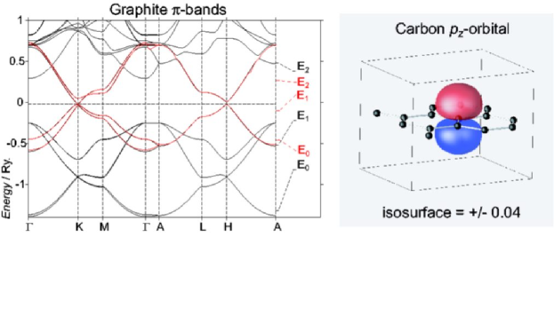
Figure 1: The band structure of graphite calculated with a full spd basis is given in black. The red bands have been calculated with a $p_{z}$ QMTO (shown on the right) on every carbon atom. The energy meshes used for each calculation are given to the right of the band structure. In all figures, red denotes a positive and blue a negative isosurface value. For the orbital plots, the isosurface values are given in units of $a_{B}^{-3/2}$, where $a_{B}$ is the Bohr radius.

It is even possible to generate orbitals for just the occupied or unoccupied $\pi$ bands in graphite. In this case we only want to pick half of the bands, and therefore we need a basis with, say, a $p_{z}$ orbital on every second carbon atom with all other partial waves being downfolded, i.e. passive. Moreover, an energy mesh spanning the bonding (anti-bonding) bands must be used in order to obtain the bonding (anti-bonding) $\pi$ orbital for graphite. Thus, the choice of the energy mesh determines which set, bonding or anti-bonding, is chosen. In Figures 2 and 3 the orbital on the central carbon atom is shown, along with the band structures computed with a full spd basis (in black) and those with the truly-minimal basis set we have just specified (in red). The agreement between the two sets of bands is excellent, with only minor deviations in the upper regions of the downfolded band structure of the anti-bonding bands where hybridization with the next higher bands occurs. Inspection of the $\pi$-bonding and anti-bonding orbitals shows that they spread out onto the first nearest-neighbour carbon atoms (passive), but they are confined not to have any $p_{z}$ character on those carbon atoms, e.g. the second nearest neighbours, where the basis set has orbitals (active partial waves). The third nearest neighbour atoms also have all partial waves downfolded and some $p_{z}$ character may be seen. Clearly, this choice of orbitals breaks the symmetry; the same Hilbert space would have been obtained had the orbitals been placed on the other half of the carbon atoms.

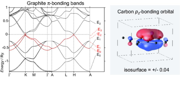
Figure 2: As in the previous figure, but the red bands have now been calculated with a $p_{z}$ Cubic-MTO (shown on the right) on every second atom within a single graphene sheet. The energy mesh is chosen within the occupied part of the $\pi$-band, which is therefore selected.

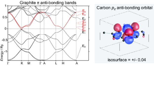
Figure 3: As in the previous figure, but the energy mesh is now in the empty part of the $\pi$-band.

It is also possible to describe the $sp^{2}$-bonding bands in graphite by placing an $s$, $p_{x}$ and $p_{y}$ orbital on every second carbon atom, downfolding all other channels and using an energy mesh which spans the energy range of the bands of interest. The band structure obtained with this basis is given in red in Figure 4 and is identical, on the scale of the figure, to the black bands which have been calculated using a full spd basis set on every carbon atom. The orbitals may spread out onto the nearest neighbour carbons, however are confined not to have any $s$, $p_{x}$ or $p_{y}$ character on the second nearest neighbours. Symmetrical orthonormalization of these three orbitals gives the well known bond orbital, the carbon $sp^{2}$ NMTO, also shown in the figure.

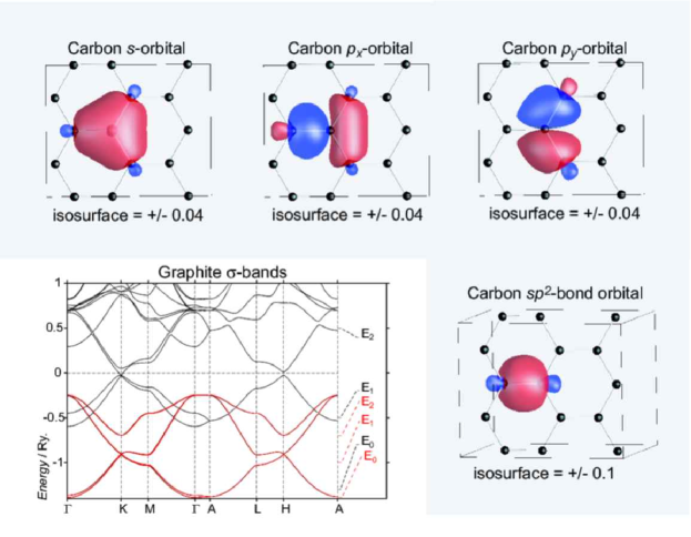
Figure 4: As in the previous figures, but the red bands have now been calculated with an $s,p_{x}$ and $p_{y}$ QMTO on every second carbon atom (shown above the band structure). Also shown is one of the three congruent $sp^{2}$-bond orbitals which arise by symmetrical orthonormalization of the $s,p_{x}$ and $p_{y}$ orbitals.

The above examples show that it is possible to describe a chosen band, or set of bands, with a truly minimal basis set consisting of one NMTO per band. Moreover, the NMTOs obtained from our method are in-line with an intuitive chemical picture of bonding in the solid state, except that they may break the symmetry. This arbitrariness originating in the constraint that the NMTOs be atom-centered can be removed by forming linear combinations of maximally localized Wannier functions. Hence, NMTOs should be useful not only, for example, as basis sets in linear scaling methods, but also in gaining a chemical understanding of periodic systems.

3.2 Boron Nitride: an insulator

The bonding in boron nitride is similar to that in graphite: within a single layer the s, $p_{x}$ and $p_{y}$ boron and nitrogen orbitals hybridize to form sp² $\sigma$-bonding and -antibonding bands. The alternation, however, makes the system insulating with a band gap between the bonding and anti-bonding $\pi$-bands. In order to describe the occupied bands, it is possible to generate either boron or nitrogen centered NMTOs. It can be expected that the electron density, and hence the orbital at a given isosurface, should have a maximum closer to the more electronegative element, nitrogen. The method needs to do less ’work’ if the orbitals are placed initially where the electrons are thought to be. Thus, we first place all the orbitals on nitrogen, and let the method shape them accordingly. This choice of atom-centered orbitals corresponds to the extreme ionic limit, a B³⁺N^3- configuration. The bonding $\sigma$ and $\pi$-bands and their respective NMTOs are shown in the top and bottom part of Figure 5, respectively. The $s,p_{x}$ and $p_{y}$ NMTOs are not shown, since they are very similar to those obtained for graphite. The full band structure is in excellent agreement with previous calculations. [18]

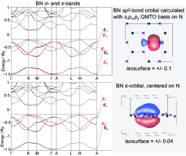
Figure 5: The band structure of boron nitride calculated with a full spd basis is given in black. The red $\sigma$-bonding bands in the upper panel have been calculated with an $s,p_{x}$ and $p_{y}$ QMTO on all nitrogen atoms, and the red $\pi$-bonding bands in the bottom panel with a $p_{z}$ orbital on all nitrogen atoms. Also given is one of the three equivalent $sp^{2}$-bond orbitals and the $p_{z}$ LMTO. Boron atoms are purple, nitrogen black.

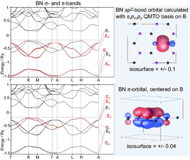
Figure 6: As in the previous figure, but with boron-centered $\sigma$ and $\pi$ basis sets.

In new materials where the bonding is not well understood, it may be difficult to decide where the orbitals should be placed. In the following we will show that NMTOs are forgiving: even a bad starting guess can yield the correct bands and Hilbert space. Placing all the orbitals on the boron atoms (a B^5-N⁵⁺ configuration) yields the bands and orbitals shown in Figure 6. The $sp^{2}$-bond orbital looks identical to the one shown in Figure 5, as it should be when the energy mesh is converged. For the $\pi$-bands, more energy points are necessary since the orbital has to spread out from a central boron onto three neighboring nitrogens. Inspection of the boron (nitrogen) centered $\pi$-NMTOs makes it plausible that when squared and summed over all boron (nitrogen) sites, they give the same electron density, with maxima shifted towards nitrogen.

3.3 Cesium: a metal

Within this section we will demonstrate that it is even possible to generate Wannier-like functions that span only the occupied bands of a metal. For lack of space, we must leave it to the reader to generalize our TB model for benzene to the corresponding model for the infinite, slightly dimerized chain, and then to study what happens for vanishing dimerization.

We shall first look at the convergence of the orbital with respect to the size of the supercell used. Whereas we can only hope to reproduce the long-ranged Friedel oscillations for supercells so large that the facets of the folded-in Brillouin zone resemble those of the Fermi surface, much smaller cells turn out to reproduce the rough shape of the occupied orbital. This is a manifestation of what Walter Kohn named the ”nearsightedness” of the electronic structure of matter. [19] We shall specifically consider cesium because of the interesting chemical aspect that its $s$-electron transforms into a $d$-electron under hydrostatic pressure.

The band structure of cesium at ambient conditions (Cs-I) calculated with a full sd basis set on every atom is given in Figure 7 in black. Superimposed on it in red is the band calculated with one s orbital on every second cesium atom, obtained specifically by breaking the symmetry and treating Cs metal as CsCl-structured Cs⁺Cs${}^{-}.$ In most regions of the Brillouin zone the agreement between the two is good, except it is obvious that with this supercell it is not possible to describe the occupied part of the upper band along the $\Gamma$X-line. Nonetheless, the orbital can be plotted and is shown in Figure 7.

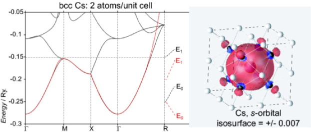
Figure 7: Band structure of bcc cesium folded into the 2 atom/cell (CsCl) simple cubic Brillouin zone. The black bands were calculated with a basis containing the $s$ and $d$ LMTOs on all atoms. The red bands were calculated with an $s$ LMTO on every second cesium atom, which is also shown. The white atoms have an $s$ orbital placed on them (active), whereas on the black atoms all partial waves are downfolded (passive).

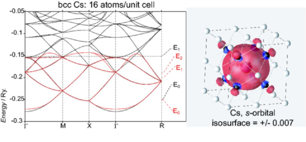
Figure 8: As in the previous figure, but for a 16-atom supercell.

The result obtained by doubling the cell in all three directions is shown in Figure 8. Now the occupied band structure has improved considerably, but is not yet perfect. The body of the orbital obtained from this calculation is, however, very similar to the one generated from the CsCl supercell. The long-ranged tail we do not monitor with the contour chosen in the figures. Already, this orbital at low isosurfaces shows the onset of $sd$-hybridization. At high isosurfaces (not shown), the orbital is completely $s$-like. The hybridization is evident in the $d_{z^{2}}$ character found on the nearest-neighbour atoms which have all partial waves downfolded, and therefore can posses any orbital character. It is a result of the fact that even though the occupied band has primarily s character, near the Fermi level some regions with $t_{2g}$ and $d_{z^{2}}$ character can be found.

Under pressure, cesium undergoes a variety of interesting structural phase transitions. At 2.3 GPa Cs-I (bcc cesium) transforms to an fcc phase.[20] Until recently, it was believed that Cs-II undergoes an isostructural transition to Cs-III (which is found in a very narrow pressure range between $\sim$4.2 and $\sim$4.3 GPa). However, experiments have shown that Cs-III has a very complicated structure which is orthorhombic (space group $C222_{1}$ with 84 atoms per unit cell).[21] At $\sim$4.3GPa Cs-III transforms to the non-close-packed tetragonal Cs-IV [22] which at $\sim$12GPa undergoes a transition to orthorhombic Cs-V [23] and finally to the double hexagonal close packed Cs-VI at $\sim$70GPa. [24] These structural transitions are beleived to be driven by the pressure-induced $s\rightarrow d$ valence electron transition. [25] Here we will generate NMTOs for Cs-II and Cs-IV in order to visualize how the valence $s$ orbital in cesium changes with increased pressure.

The occupied bands for Cs-II with $v/v_{0}=$ 0.6 are still primarily $s$-like, however a fair amount of $e_{g}$-character can also be found. Upon increasing pressure, a Lifshitz transition occurs (change in the topology of the Fermi surface) as higher lying $t_{2g}$ bands cross the Fermi level. Figure 9 shows the band structure of Cs-II for a 32-atom supercell compressed past the calculated volume of the Lifshitz transition. The agreement between the downfolded and full band structures is excellent and the downfolded bands are even able to describe the aforementioned $t_{2g}$ bands. The orbital at high isosurfaces is clearly no longer $s$-like. It must be noted that the orbital calculated for $v/v_{0}=$ 0.6, using the same supercell and downfolding scheme, yielded a very similar orbital (not shown), the only difference being that the four lobes evident in Figure 9 are located in the same plane.

Figure 9: As in the previous figure, but for fcc cesium with $v/v_{0}=$ 0.4, and a 32-atom supercell.

Cs-IV with each cesium atom having a coordination of 8 is no longer a close-packed structure. It can be viewed as a stacking of prisms with a ninety degree rotation from layer to layer in the $c$-direction. The TB-LMTO calculated charge density (Figure 10) shows maxima in the interstitial regions, in the center of these prisms. The LMTO obtained by placing one $s$-orbital on every second cesium atom and downfolding all other partial waves is given in Figure 10. Clearly this orbital can be obtained from that shown in Figure 9 by raising two and lowering two of the lobes. Placing the Cs-IV LMTO on all of the active sites and squaring it yields a charge density which is almost identical to that calculated with TB-LMTO, [26] giving further validation that our method works. Thus we have shown that $N$MTOs may be used to give a chemical picture of the pressure induced electronic phase transition in cesium yielding results which are in-line with those obtained from standard electronic structure calculations.

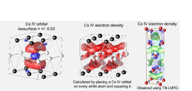
Figure 10: The LMTO obtained for Cs-IV ($v/v_{0}=$ 0.316) with 2-atoms/cell. An $s$ orbital was placed on all white atoms (active), whereas the partial waves on the black atoms were downfolded (passive). Also shown is the charge density obtained by placing the LMTO on every white atom and squaring it, along with the charge density obtained from a TB-LMTO calculation. The latter charge density is colored by the ELF. The isosurface taken is 0.0063 $a_{B}^{-3}$.

4 Summary and conclusions

Within this article we have shown that the $3^{rd}$ generation MTO method can be used to design a basis set of atom-centered localized orbitals, which span the wave functions in a given energy range. For an isolated set of bands, arbitrary accuracy may be obtained, with only one basis function per electron pair (or single electron, in the case of spin-polarized calculations), simply by increasing the density of the energy mesh which spans the energy range of the band in question. This method may be applied to insulating and even metallic systems to generate Wannier-like functions which are in-line with a chemical understanding of bonding in the solid-state. It should therefore be a useful analysis tool in, for example, explaining experimental trends for a given set of compounds via orbital based arguments; clarifying the bonding in novel or even amorphous materials; visualizing pressure-driven electronic transitions.

$3^{rd}$ generation MTOs may also be useful in generating truly-minimal basis sets for order-N methods and in constructing many-electron wave functions which can be applied to study strongly correlated systems realistically. In our implementation, NMTOs are generated using the self-consistent potential from an LMTO calculation. However, our method may be interfaced with the results of any other program, providing that the potential can be expressed in terms of a superposition of spherically symmetric potential wells with radial overlaps of up to $\sim$60 percent.

5 Computational Methods

Graphite has a hexagonal unit cell. The space group is P6₃/mmc (194) and the two basis carbon atoms are located in the $2b$ and $2c$ Wyckoff positions. The lattice constants, a and c were taken from experimental data [27] as being 2.4642 Å and 6.7114 Å, respectively. In addition to the atoms on the two crystallographic positions, it was necessary to insert two interstitial spheres to represent the charge density in the calculation.

Boron nitride is also found with space group P6₃/mmc (194), with the boron atom located in the $2c$ and the nitrogen atom in the $2d$ Wykoff positions. The lattice constants, a and c were taken from experimental data [28] as being 2.50399 Å and 6.6612 Å, respectively. It was only necessary to insert one interstitial sphere.

At ambient conditions, cesium crystalizes in the bcc structure. Calculations were performed using the experimental lattice parameter of 6.048 Å. [29] Cs-II is fcc and the bands shown here were calculated for $v/v_{0}=$ 0.4. Both Cs-I and Cs-II are close-packed so it was not necessary to insert any empty spheres. Cs-IV has the space group I4₁/amd with 2 atoms per unit cell [22] and it was necessary to insert four empty spheres.

All of the TB-LMTO calculations [26] were performed using the Vosko-Wilk-Nusair (VWN) LDA [30] along with the Perdew-Wang GGA. [31] Scalar relativistic effects were included. For graphite and boron nitride a basis set consisting of $spd$ LMTOs on the carbon, boron and nitrogen atoms with $sp$ LMTOs on the empty spheres, was used. For cesium, the basis consisted of $sd$ LMTOs with $pf$ LMTOs being downfolded. For graphite and boron nitride, the calculations utilized 1953 irreducible points in the tetrahedron k-space integrations,[32] 1661 and 897 points were used in the calculation for cesium in the bcc and fcc structures (one atom per unit cell), respectively, and 693 points were used in the calculation for Cs-IV.

The present version of the NMTO program is not self-consistent and requires the output of the self-consistent potential from the TB-LMTO program. The downfolded band structures are compared with bands computed employing a full NMTO basis set; not with those obtained using the TB-LMTO program. In all cases, the default values for the hard-sphere radii, $a_{R}$, were used. Thus, all of the hard spheres were slightly smaller than touching. However in general, the $a_{R}$ should be taken as 0.9 times the tabulated covalent, atomic or ionic radii. In the calculations all partial-waves on the empty spheres were downfolded. The other downfolding schemes and energy meshes employed for particular calculations are given in the results and discussion section of the paper. Note that a mesh employing two (N+1=2) energy points yields a linear-MTO or LMTO, one with three points a quadratic-MTO or QMTO, and so on. More details about the NMTO formalism can be found in [7, 9, 8] and references within.

References

- [1] R. Car and M. Parrinello. Phys. Rev. Lett., 55:2471, 1997.
- [2] S. F. Boys. Revs. Modern Phys., 32:296, 1960.
- [3] N. Marzari and D. Vanderbilt. Phys. Rev. B., 56:12847, 1997.
- [4] P. L. Silvestrelli, N. Marzari, D. Vanderbilt, and M. Parrinello. Solid State Communications, 107:7, 1998.
- [5] M. Boero, M. Parrinello, S. Hüffer, and H. Weiss. J. Am. Chem. Soc., 122:501, 2000.
- [6] O. K. Andersen, T. Saha-Dasgupta, R. W. Tank, C. Arcangeli, O. Jepsen, and G. Krieg. Electronic Structure and Physical Properties of Solids. The Uses of the LMTO Method. (Lecture notes in Physics, vol. 535). Springer, Berlin/Heidelberg, 2000.
- [7] O. K. Andersen and T. Saha-Dasgupta. Phys. Rev. B., 62(24):R16219, 2000.
- [8] R. W. Tank and C. Arcangeli. Phys. Stat. Sol.(b), 217:89, 2000.
- [9] O. K. Andersen, T. Saha-Dasgupta, and S. Ezhov. Bull. Mater. Sci., 26:19, 2003.
- [10] E. Pavarini, S. Biermann, A. Poteryaev, A. I. Lichtenstein, A. Georges, and O. K. Andersen. Phys. Rev. Lett., 92:176403, 2004.
- [11] T. F. A. Müller, V. Anisimov, T. M. Rice, I. Dasgupta, and T. Saha-Dasgupta. Phys. Rev. B., 57:R12655, 1998.
- [12] R. Valenti, T. Saha-Dasgupta, J. V. Alvarez, K. Požgajčić, and C. Gros. Phys. Rev. Lett., 86:5381, 2001.
- [13] E. Pavarini, I. Dasgupta, T. Saha-Dasgupta, O. Jepsen, and O. K. Andersen. Phys. Rev. Lett., 87:047003, 2001.
- [14] A. J. Williamson, R. Q. Hood, and J. C. Grossman. Phys. Rev. Lett., 87:246406, 2001.
- [15] A. J. Williamson, J. C. Grossman, R. Q. Hood, A. Puzder, and G. Galli. Phys. Rev. Lett., 89:196803, 2002.
- [16] W. Kohn and J. Rostocker. Phys. Rev., 94:111, 1954.
- [17] R. Ahuja, S. Auluck, J. Trygg, J. M. Wills, O. Eriksson, and B. Johansson. Phys. Rev. B., 51:4813, 1995.
- [18] A. Catellani, M. Posternak, A. Baldereschi, and A. J. Freeman. Phys. Rev. B., 36:6105, 1987.
- [19] W. Kohn. Phys. Rev. Lett., 76:3168, 1996.
- [20] H. T. Hall, L. Merrill, and J. D. Barnett. Science, 146:1297, 1964.
- [21] M.I. McMahon, R.J. Nelmes, and S. Rekhi. Phys. Rev. Lett., 87:255502, 2001.
- [22] K. Takemura, S. Minomura, and O. Shimomura. Phys. Rev. B, 49:1772, 1982.
- [23] U. Schwarz, K. Takemura, M. Hanfland, and K. Syassen. Phys. Rev. Lett., 81:2711, 1998.
- [24] K. Takemura, N. E. Christensen, D. L. Novikov, K. Syassen, U. Schwarz, and M. Hanfland. Phys. Rev. B, 61:14399, 2000.
- [25] R Sternheimer. Phys. Rev., 78:235, 1950.
- [26] O. K. Andersen and O. Jepsen. Phys. Rev. Lett., 53(27):2571, 1984.
- [27] P. Trucano and R. Chen. Nature, 258(258):136, 1975.
- [28] R. S. Pease. Acta Crystallographica, 5:356, 1952.
- [29] M. S. Anderson, E. J. Gutman, J. R. Packard, and C. A. Swenson. J. Phys. Chem. Solids, 30:1587, 1969.
- [30] S. H. Vosko, L. Wilk, and M. Nusair. Can. J. Phys., 58(8):1200, 1980.
- [31] J. P. Perdew and Y. Wang. Phys. Rev. B., 33(33):8800, 1986.
- [32] P. E. Blöchl, O. Jepsen, and O. K. Andersen. Phys. Rev. B., 49(49):16223, 1994.