Violation of the Fluctuation-Dissipation Theorem and Heating Effects in the Time-Dependent Kondo Model

Abstract

The fluctuation-dissipation theorem (FDT) plays a fundamental role in understanding quantum many-body problems. However, its applicability is limited to equilibrium systems and it does in general not hold in nonequilibrium situations. This violation of the FDT is an important tool for studying nonequilibrium physics. In this paper we present results for the violation of the FDT in the Kondo model where the impurity spin is frozen for all negative times, and set free to relax at positive times. We derive exact analytical results at the Toulouse point, and results within a controlled approximation in the Kondo limit, which allow us to study the FDT violation on all time scales. A measure of the FDT violation is provided by the effective temperature, which shows initial heating effects after switching on the perturbation, and then exponential cooling to zero temperature as the Kondo system reaches equilibrium.

I Introduction

The fluctuation-dissipation theorem (FDT)CW is of fundamental importance for the theoretical understanding of many-body problems. It establishes a relation between the equilibrium properties of a system and its response to an external perturbation. In nonequilibrium situations this powerful tool is in general not available: typical nonequilibrium situations are e.g. systems prepared in an excited state, or systems driven into an excited state by pumping energy into them. Since such nonequilibrium systems occur everywhere in nature, the investigation of nonequilibrium many-body physics has become one of the key challenges of modern theoretical physics. The violation of the FDT in a nonequilibrium system plays an important role in such studies as it characterizes “how far” the system is driven out of equilibrium.

Most widely investigated in this context are glassy systems, that is systems with a very long relaxation time compared to the typical time scale of measurements. Due to the long relaxation times it is experimentally possible to measure the deviation from the FDT, i.e. to study the ageing effects: one observes a relaxation of the nonequilibrium initial state towards equilibrium. For a review of this field see Refs. HertzFisher, ; Calabrese_review, .

However, these are classical systems at finite temperature and therefore the classical limit of the FDT is studied. Nonequilibrium zero temperature quantum systems provide a very different limit which has been studied very little in the literature (however, see Ref. Mauger, ). This is one of the main motivations for our work which looks at the FDT violation in the time-dependent Kondo model at zero temperature. Time-dependence is here introduced by freezing the impurity spin at negative times, and then allowing it to relax at positive times. Besides being of fundamental theoretical importance as the paradigm for strong-coupling impurity physics in condensed matter theory, Kondo physics is also experimentally realizable in quantum dots. The Kondo effect has been observed in quantum dot experimentsKondo_dots , and time-dependent switching of the gate potential amounts to a realization of the time-dependent Kondo modelNordlander which should be possible in future experiments.

Our calculations here are based on recent work on the time-dependent Kondo model with exact analytical results for the Toulouse point and results in a controlled approximation in the experimentally relevant Kondo limit.article We will see that the FDT is maximally violated at intermediate time scales of order the inverse Kondo temperature: the effective temperature becomes of order the Kondo temperature due to heating of the conduction band electrons by the formation of the Kondo singlet. The system then relaxes towards equilibrium and the FDT becomes fulfilled exponentially fast at larger times.

II Fluctuation-Dissipation Theorem

Consider an observable $A$ which is coupled linearly to a time-dependent external field $h(t)$. The Hamiltonian of the system is then given by

$$H=H_{0}-h(t)\,A\ ,$$ (1)

where $H_{0}$ is the unperturbed part of the Hamiltonian. The generalized susceptibility (or response) $R(t,t^{\prime})$ of the observable $A$ at time $t$ to the external small perturbation $h(t^{\prime})$ at time $t^{\prime}$ is defined as

$$R(t,t^{\prime})=\left.\frac{\delta\langle\overline{A(t)}\rangle}{\delta h(t^{\prime})}\right|_{h=0}\ .$$ (2)

Here $\langle\overline{A(t)}\rangle\equiv\langle A(t)\rangle_{h}-\langle A(t)\rangle_{0}$ is the deviation of the expectation value from its equilibrium value. If the system is in equilibrium before its perturbation by the field $h$, then $R(t,t^{\prime})$ depends only on the time difference $\tau=t-t^{\prime}$. One introduces the Fourier transform of $R(\tau)$

$$R(\omega)=\int_{0}^{\infty}R(\tau)e^{i\omega\tau}d\tau\ ,$$ (3)

where the integration runs only over positive times as a consequence of causality. A simple calculation shows that the imaginary part of $R(\omega)$ is proportional to the energy dissipated by the system for a small periodic perturbation with frequency $\omega$ (see, for example, Ref. LL, ). Thus the response function determines the dissipation properties of the equilibrium system.

For calculating the response function one defines the two-time correlation function

$$C_{A,A}(t,t^{\prime})\equiv\left\langle A(t)A(t^{\prime})\right\rangle=\frac{1}{Z}Tr\left[A(t)A(t^{\prime})\rho\right]\ ,$$ (4)

with the operators in the Heisenberg picture

$$A(t)\equiv\exp\left(iHt\right)A(0)\exp\left(-iHt\right)\ .$$ (5)

The trace runs over all the states in the Hilbert space, $\rho$ is the density matrix and $Z$ the partition function. Symmetrized and antisymmetrized correlation functions $C_{\left\{A,A\right\}}(t,t^{\prime})$, $C_{\left[A,A\right]}(t,t^{\prime})$ are defined in the same way

$$C_{\left\{A,A\right\}}(t,t^{\prime}) \equiv \frac{1}{2}\left\langle\left\{A(t),A(t^{\prime})\right\}\right\rangle$$ (6)

$$C_{\left[A,A\right]}(t,t^{\prime}) \equiv \frac{1}{2}\left\langle\left[A(t),A(t^{\prime})\right]\right\rangle\ .$$ (7)

The cumulant of the symmetrized correlation function is

$$C^{\rm(cum)}_{\{A,A\}}(t,t^{\prime})\equiv C_{\{A,A\}}(t,t^{\prime})-\langle A(t)\rangle\,\langle A(t^{\prime})\rangle\ .$$ (8)

In the framework of linear response theory (that is for small perturbations) one then proves the famous Kubo formulaKubo

$$R(t,t^{\prime})=2i\theta(t-t^{\prime})C_{\left[A,A\right]}(t,t^{\prime})\ .$$ (9)

Here the time dependence of all operators is given by the unperturbed part of the Hamiltonian $H_{0}$. Since in equilibrium all correlation functions depend only on the time difference $\tau=t-t^{\prime}$, one defines their Fourier transform with respect to $\tau$

$$C^{\rm(cum)}_{\{A,A\}}(\omega)=\int_{-\infty}^{\infty}C^{\rm(cum)}_{\{A,A\}}(\tau)\,e^{i\omega\tau}d\tau\ .$$ (10)

If the initial state is the equilibrium state for a given temperature, $R(\omega)$ and $C^{\rm(cum)}_{\{A,A\}}(\omega)$ are related by the famous Callen-Welton relationCW , which is also known as $the$ Fluctuation-Dissipation theorem

$${\rm Im}\,R(\omega)=\tanh\left(\frac{\beta\omega}{2}\right)C^{\rm(cum)}_{\{A,A\}}(\omega)\ .$$ (11)

Here $\beta$ is the inverse temperature. For $T=0$ Eq. (11) reads

$${\rm Im}\,R(\omega)={\rm sgn}\left(\omega\right)C^{\rm(cum)}_{\{A,A\}}(\omega)\ .$$ (12)

Eqs. (11) and (12)footnote_cumulant relate dissipation with equilibrium fluctuations, which is the fundamental content of the FDT.

III FDT Violation in Nonequilibrium

Let us recapitulate why the FDT (11) in general will not hold in quantum nonequilibrium systems. We will only consider the zero temperature case since it brings out the quantum effects most clearly; the generalization to nonzero temperatures is straightforward.

We first consider how a typical experiment is actually performed: the system in prepared in some initial state at time $t=0$ (not necessarily its ground state) and then evolves according to its Hamiltonian. A response measurement is then done by applying the external field after a waiting time $t_{w}>0$, and the response to this is measured a time difference $\tau$ later. The Fourier transform with respect to (positive) time difference will then in general depend on the waiting time $t_{w}$

$$R(\omega,t_{w})=\int_{0}^{\infty}R(t_{w}+\tau,t_{w})\,e^{i\omega\tau}d\tau\ .$$ (13)

Likewise in an experimental measurement of the correlation function the first measurement of the observable will be performed after the waiting time $t_{w}$, and then at time $t_{w}+\tau$ the second measurement follows. From the experimental point of view this leads again to a one-sided Fourier transform

$$C^{\rm(cum)}_{\{A,A\}}(\omega,t_{w})=2\int_{0}^{\infty}C^{\rm(cum)}_{\{A,A\}}(t_{w}+\tau,t_{w})\,\cos(\omega\tau)d\tau\ .$$ (14)

If the system is prepared in its ground state, or if the system equilibrates into its ground state for sufficiently long waiting time $t_{w}\rightarrow\infty$, then we can replace this one-sided Fourier transform by the symmetric version and arrive at the conventional equilibrium definition (10).

However, for a nonequilibrium preparation at $t=0$ Eqs. (13) and (14) are the suitable starting point for the discussion of the FDT (12). Let us therefore look at the FDT in the framework of (13) and (14). We follow the standard derivationLL and introduce a complete set of eigenstates $|n\rangle$ of the Hamiltonian $H$, $H|n\rangle=E_{n}|n\rangle$. The matrix elements of the operator $A$ are denoted by $A_{nm}=\langle n|A|m\rangle$ in this basis. Then a matrix element of the susceptibility is given by

$$R(t,t_{w})_{nn^{\prime}}=i\theta(t-t_{w})\sum_{m}A_{nm}A_{mn^{\prime}}$$

$$\!\!\times\left(e^{i(E_{n}-E_{m})t}e^{i(E_{m}-E_{n^{\prime}})t_{w}}-e^{i(E_{n}-E_{m})t_{w}}e^{i(E_{m}-E_{n^{\prime}})t}\right)$$

The imaginary part of (13) is

$${\rm Im}\,R(\omega,t_{w})_{nn^{\prime}}={\rm Re}\>\sum_{m}A_{nm}A_{mn^{\prime}}$$

$$\times\int_{0}^{\infty}\left(e^{i\omega_{nm}\tau}-e^{i\omega_{mn^{\prime}}\tau}\right)e^{i\omega_{nn^{\prime}}t_{w}}e^{i\omega\tau}d\tau$$

with $\omega_{nm}\equiv E_{n}-E_{m}$. For diagonal matrix elements $n=n^{\prime}$ this implies

$${\rm Im}\,R(\omega,t_{w})_{nn}=$$

$$\frac{1}{2}\sum_{m}A_{nm}A_{mn}\left(\delta(\omega+\omega_{nm})-\delta(\omega+\omega_{mn})\right)\ .$$

Likewise for the correlation function

$$C_{\{A,A\}}(\omega,t_{w})_{nn^{\prime}}=\sum_{m}A_{nm}A_{mn^{\prime}}$$

$$\times\int_{0}^{\infty}\left(e^{i\omega_{nm}\tau}+e^{i\omega_{mn^{\prime}}\tau}\right)e^{i\omega_{nn^{\prime}}t_{w}}\cos(\omega\tau)d\tau$$

and the diagonal matrix elements are

$$C^{\rm(cum)}_{\{A,A\}}(\omega,t_{w})_{nn}=$$

$$\frac{1}{2}\sum_{m\neq n}A_{nm}A_{mn}\left(\delta(\omega+\omega_{nm})+\delta(\omega+\omega_{mn})\right)\ .$$

If we take $|n\rangle=|{\rm GS}\rangle$ as the ground state of our Hamiltonian, i.e. the system is in equilibrium, then we know $\omega_{nm}=E_{\rm GS}-E_{m}\leqslant 0$ and $\omega_{mn}=E_{m}-E_{\rm GS}\geqslant 0$ for all $m$. For positive $\omega$ therefore only the first terms in (III) and (III) contribute, and for negative $\omega$ the second terms contribute: this just proves the zero temperature FDT (12) with its sgn($\omega$)-coefficient.

Now let us assume the nonequilibrium situation described above where the system is prepared in some arbitrary initial state $|{\rm NE}\rangle$ at $t=0$. One can expand $|{\rm NE}\rangle$ in terms of the eigenstates $|n\rangle$ of the Hamiltonian

$$|{\rm NE}\rangle=\sum_{n}c_{n}|n\rangle$$ (20)

with suitable coefficients $c_{n}$. Then the relations (III) and (III) are modified like

$${\rm Im}\,R(\omega,t_{w})_{\rm NE} = \sum_{m,n,n^{\prime}}c^{*}_{n}c^{\phantom{\dagger}}_{n^{\prime}}A_{nm}A_{mn^{\prime}}\times\ldots$$

$$C_{\{A,A\}}(\omega,t_{w})_{\rm NE} = \sum_{m,n,n^{\prime}}c^{*}_{n}c^{\phantom{\dagger}}_{n^{\prime}}A_{nm}A_{mn^{\prime}}\times\ldots\ ,$$

where ”$\ldots$” stands for the same expressions as in (III) and (III). In general this will lead to a nonzero difference

$${\rm sgn(\omega)}\,C^{\rm(cum)}_{\{A,A\}}(\omega,t_{w})_{NE}-{\rm Im}\,R(\omega,t_{w})_{NE}\not=0$$ (21)

and therefore the FDT is violated. We will next study the violation of the FDT explicitly in the time-dependent Kondo model, and in particular also show that the difference (21) vanishes exponentially fast for large waiting times $t_{w}$.

IV Time-Dependent Kondo Model

We briefly review the results obtained in Ref. article, for the spin dynamics of the time-dependent Kondo model. The time-dependent Kondo model is described by the Hamiltonian

$$H=\sum_{k,\alpha}\epsilon^{\phantom{\dagger}}_{k}c^{\dagger}_{k\alpha}c^{\phantom{\dagger}}_{k\alpha}+\sum_{i}J_{i}\sum_{\alpha,\beta}c^{\dagger}_{0\alpha}\,S^{\phantom{\dagger}}_{i}\,\sigma^{\alpha\beta}_{i}\>c^{\phantom{\dagger}}_{0\beta}\ .$$ (22)

We allow for anisotropic couplings $J_{i}=(J_{\bot},J_{\bot},J_{\|})$ and consider a linear dispersion relation $\epsilon_{k}=v_{F}\,k$. We have studied two nonequilibrium preparations in Ref. article, : I) The impurity spin is frozen for time $t<0$ by a large magnetic field term $h(t)S_{z}$ that is switched off at $t=0$: $h(t)\gg T_{\rm K}$ for $t<0$ and $h(t)=0$ for $t\geq 0$. II) The impurity spin is decoupled from the bath degrees of freedom for time $t<0$ (like in situation I we assume $\langle S_{z}(t\leq 0)\rangle=+1/2$) and then the coupling is switched on at $t=0$: $J_{i}(t)=0$ for $t<0$ and $J_{i}(t)=J_{i}>0$ time-independent for $t\geq 0$. For both scenarios the impurity spin dynamics could then be described by an effective time-dependent resonant-level Hamiltonian in terms of fermionic solitons $\Psi_{k}$ consisting of spin-density excitations:

$$H=\sum_{k}\varepsilon^{\phantom{\dagger}}_{k}\Psi_{k}^{{\dagger}}\Psi^{\phantom{\dagger}}_{k}+\left\{\begin{array}[]{lc}\sum\limits_{kk^{\prime}}g_{kk^{\prime}}\,\Psi_{k}^{{\dagger}}\Psi^{\phantom{\dagger}}_{k^{\prime}}(d^{{\dagger}}d-1/2)&,\,t<0\\ &\\ \sum\limits_{k}V^{\phantom{\dagger}}_{k}(\Psi^{{\dagger}}_{k}d+d^{{\dagger}}\Psi^{\phantom{\dagger}}_{k})&,\,t>0\end{array}\right.$$ (23)

with effective parameters $g_{kk^{\prime}}$ and $V_{k}$ (which also depend on scenario I or II). The impurity spin $S_{z}$ is given by $S_{z}=d^{{\dagger}}d-1/2$. Since the effective Hamiltonian is quadratic for both negative and positive times, it is straightforward to find an explicit solution for the impurity orbital correlation functions and work out their dependence on the waiting time. Detailed inspectionarticle shows that the impurity spin dynamics is the same for both nonequilibrium initial preparations I and II.

V Toulouse Point

At the Toulouse pointToulouse with $J_{\|}/2\pi v_{F}=1-1/\sqrt{2}$ the mapping to the effective resonant level model (23) is exact and the effective parameters $g_{kk^{\prime}}$ and $V_{k}$ are independent of $k,k^{\prime}$. This allowed us to express the spin-spin correlation functions in closed analytical formarticle

$$C^{\rm(cum)}_{\{S_{z},S_{z}\}}(\tau,t_{w})\stackrel{{\scriptstyle\rm def}}{{=}}$$

$$= \frac{1}{2}\,\langle\,\{S_{z}(t_{w}),S_{z}(t_{w}+\tau)\,\}\rangle-\langle S_{z}(t_{w})\rangle\,\langle S_{z}(t_{w}+\tau)\rangle$$

$$= \frac{1}{4}e^{-2\tau/t_{\rm B}}(1-e^{-4t_{w}/t_{\rm B}})$$

$$-\left(s(\tau)-s(t_{w}+\tau)e^{-t_{w}/t_{\rm B}}+s(t_{w})e^{-(t_{w}+\tau)/t_{\rm B}}\right)^{2}$$

for the symmetrized part and

$$C_{[S_{z},S_{z}]}(\tau,t_{w})\stackrel{{\scriptstyle\rm def}}{{=}}\frac{1}{2}\,\langle\,[S_{z}(t_{w}),S_{z}(t_{w}+\tau)]\,\rangle$$ (25)

$$= -i\,e^{-\tau/t_{\rm B}}\Big{(}s(\tau)-s(t_{w}+\tau)e^{-t_{w}/t_{\rm B}}$$

$$\qquad\qquad+s(t_{w})e^{-(t_{w}+\tau)/t_{\rm B}}\Big{)}$$

for the antisymmetrized part. Here $s(t)\stackrel{{\scriptstyle\rm def}}{{=}}(t_{\rm B}/\pi)\int_{0}^{\infty}d\omega\,\sin(\omega\tau)/(1+\omega^{2}t_{\rm B}^{2})$ with the shorthand notation $t_{\rm B}=\pi wt_{\rm K}$. $w=0.4128$ is the Wilson number and $t_{\rm K}=1/T_{\rm K}$ is the Kondo time scale, i.e. the inverse Kondo temperature. In this paper we use the definition of the Kondo temperature $T_{\rm K}$ via the zero temperature impurity contribution to the Sommerfeld coefficient, $\gamma_{\rm imp}=w\pi^{2}/3T_{\rm K}$.

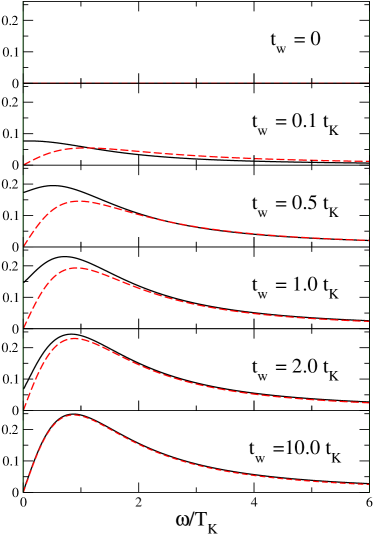
Figure 1: Universal curves for the spin-spin correlation function $T_{\rm K}\times C^{\rm(cum)}_{\{S_{z},S_{z}\}}(\omega,t_{w})$ (solid line) and response function $T_{\rm K}\times\,{\rm Im}\,R(\omega,t_{w})$ (dashed line) at the Toulouse point. Notice the normalization of the equilibrium curve ($t_{w}\rightarrow\infty$) which follows from (6) with the operator identity $S_{z}^{2}=1/4$: this gives $\int_{0}^{\infty}C^{\rm(cum)}_{\{S_{z},S_{z}\}}(\omega,t_{w}=\infty)d\omega=\pi/4$.

From (V) and (25) one can obtain the Fourier transforms (13) and (14). Results for $C^{cum}_{\{S_{z},S_{z}\}}(\omega,t_{w})$ and ${\rm Im}R(\omega,t_{w})$ for various waiting times $t_{w}$ are shown in Fig. 1. For zero waiting time $t_{w}=0$ the FDT is trivially fulfilled since the system is prepared in an eigenstate of $S_{z}$ and therefore both functions vanish identically, $C^{\rm(cum)}_{\{S_{z},S_{z}\}}(\omega,t_{w}=0)={\rm Im}\,R(\omega,t_{w}=0)=0$. For increasing waiting time the curves start to differ, which indicates the violation of the FDT in nonequilibrium. For large waiting time as compared to the Kondo time scale one can then see nicely that the curves coincide again, which shows that the system reaches equilibrium behavior for $t_{w}\rightarrow\infty$ where the FDT is known to hold. From the curves in Fig. 1 one also notices that the maximum violation of the FDT occurs at zero frequency, while it becomes fulfilled more rapidly at higher frequencies. We interpret this as showing that high-energy excitations find “equilibrium-like” behavior faster than low-energy excitations probed by the small $\omega$ response. The high-energy components of the initial nonequilibrium state can “decay” more quickly for a given waiting time.

At zero frequency $C^{\rm(cum)}_{\{S_{z},S_{z}\}}(\omega=0,t_{w})$ is non-zero for $0<t_{w}<\infty$ as if one were studying the spin dynamics of the equilibrium system at finite temperature. This leads to the definition of the effective temperature $T_{\rm eff}$ via the zero frequency limit of (11)

$$\lim_{\omega\rightarrow 0}\frac{{\rm Im}\,R(\omega)}{\omega}=\frac{1}{2T_{\rm eff}}\,C^{\rm(cum)}_{\{A,A\}}(\omega=0)\ .$$ (26)

This concept of an “effective temperature” is frequently used and well-established in the investigation of classical nonequilibrium systems.Kurchan We suggest that it is also useful in a quantum nonequilibrium system by giving a measure for the “effective temperature” of our bath (i.e. the conduction band electrons) in the vicinity of the impurity.

We can see this explicitly by using (26) to evaluate the effective temperature as a function of the waiting time; the results are shown in Fig. 2.

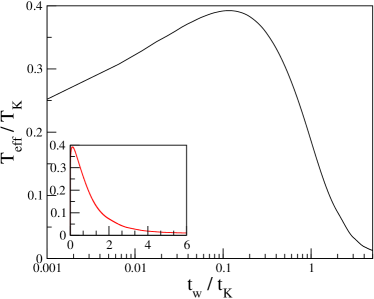
Figure 2: Effective temperature $T_{\rm eff}$ as a function of the waiting time $t_{w}$ at the Toulouse point. The inset shows the same curve on a linear scale to illustrate how fast the initial heating occurs.

One sees that the effective temperature goes up very quickly as a function of the waiting time until it reaches a maximum of $T_{\rm eff}\approx 0.4T_{\rm K}$ at $t_{w}\approx 0.1t_{\rm K}$. After that the system cools down again. We can understand this by noticing that the conduction band is initially in its ground state with respect to the Hamiltonian for $t<0$, therefore its effective temperature vanishes. As the spin dynamics is turned on at $t=0$ the Kondo singlet starts building up. Its nonzero binding energy therefore initially “heats up” the conduction band electrons. After a sufficiently long time the Kondo singlet has been formed and then the process of energy diffusion takes over: the binding energy that has initially been stored in the vicinity of the Kondo impurity diffuses away, the system equilibrates and the effective temperature goes back to zero. The behavior of the effective temperature therefore traces this competition of release of binding energy and energy diffusion away from the impurity. Analytically one can show for very small waiting time $t_{w}\ll t_{\rm K}$

$$\frac{T_{\rm eff}}{T_{\rm K}}\simeq\frac{1}{w}\frac{1}{\ln(\pi w\,t_{\rm K}/t_{w})}$$ (27)

and an exponential decay to zero temperature for long waiting time $t_{w}\gg t_{\rm K}$

$$\frac{T_{\rm eff}}{T_{\rm K}}\propto e^{-t_{w}/t_{\rm K}}\ .$$ (28)

Finally we want to emphasize that while the effective temperature seems a useful phenomenological concept for interpreting the $\omega=0$ behavior in nonequilibrium, its definition (26) does not capture the small $\omega$-behavior. Since $C^{\rm(cum)}_{\{S_{z},S_{z}\}}(\omega,t_{w})-C^{\rm(cum)}_{\{S_{z},S_{z}\}}(\omega=0,t_{w})\propto|\omega|$ is nonanalytic for small $\omega$ and finite waiting time (see Fig. 1 and the discussion in Ref. article, ), the long time decay of the spin-spin correlation function is always algebraic for all $t_{w}>0$ (therefore characteristic of equilibrium zero temperature behavior), $C^{\rm(cum)}_{\{S_{z},S_{z}\}}(\tau,t_{w})\propto\tau^{-2}$.

VI Kondo Limit

The Kondo limit with small coupling constants $J_{\perp},J_{\parallel}\rightarrow 0$ is the relevant regime for experiments on quantum dots. In this regime the results in Ref. article, are not exact, but were shown to be very accurate by comparison with asymptotically exact results for $t_{w}=0$ and $\tau/t_{\rm K}\gg 1$.LesageSaleur For our purposes here the main difference from the Toulouse point analysis is the nontrivial structure of the effective parameters $g_{kk^{\prime}}$ and $V_{k}$ from Ref. article, in (23). This makes it impossible to give closed analytic expressions like (V) or (25), but the numerical solution of the quadratic Hamiltonian (23) is still straightforward. The results presented in this section were obtained by numerical diagonalization of (23) with 4000 band states. The numerical errors from the discretization are very small (less than $2\%$ relative error in all curves).footnote_UV

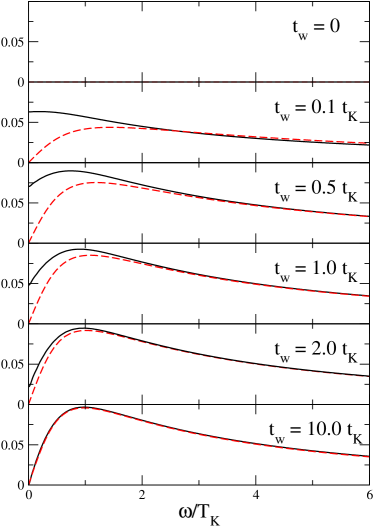
Figure 3: Universal curves for the spin-spin correlation function $T_{\rm K}\times C^{\rm(cum)}_{\{S_{z},S_{z}\}}(\omega,t_{w})$ (solid line) and response function $T_{\rm K}\times\,{\rm Im}\,R(\omega,t_{w})$ (dashed line) in the Kondo limit (compare with Fig. 1).

Fig. 3 shows the behavior of the spin-spin correlation function and the response function obtained in this manner. Similar to the Toulouse point results we observe a violation of the FDT for finite nonzero waiting time, $0<t_{w}<\infty$. For $t_{w}\rightarrow\infty$ one recovers the FDT exponentially fast (28) as expected since the system equilibrates. The results for the effective temperature in the Kondo limit are depicted in Fig. 4. While the behavior of $T_{\rm eff}(t_{w})$ is somehow more complicated than at the Toulouse point, the interpretation regarding heating and cooling effects carries over without change. The main difference is that the maximum effective temperature is already reached for $t_{w}\approx 0.03t_{K}$ in the Kondo limit. We interpret this as being due to the (dimensionful) bare coupling constants at higher energies that are larger than the renormalized low energy scale $T_{\rm K}$ and therefore lead to faster heating.

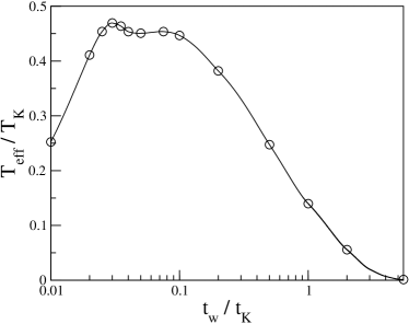
Figure 4: Effective temperature $T_{\rm eff}$ as a function of the waiting time $t_{w}$ in the Kondo limit. The line is a guide to the eye. The size of the datapoints (circles) indicates the numerical error. The datapoint for $t_{w}/t_{\rm K}=5.5$ is numerically indistinguishable from zero.

VII Conclusions

Our investigation of the zero temperature quantum limit of the fluctuation-dissipation theorem in the time-dependent Kondo model provides some important lessons regarding its relevance in quantum nonequilibrium systems. For the Kondo system prepared in an initial state with a frozen impurity spin, i.e. in a product state of system and environment, the FDT is violated for all nonzero waiting times $t_{w}$ of the first measurement after switching on the spin dynamics at $t=0$. For large waiting times as compared to the Kondo time scale the FDT becomes fulfilled exponentially fast, which indicates the quantum equilibration of the Kondo system. A quantitative measure for the violation of the FDT is provided by the effective temperature $T_{\rm eff}$Kurchan here defined via the spin dynamics (26) and depicted in Figs. 2 and 4. It traces the buildup of fluctuations in the conduction band: Initially, the conduction band electrons are in equilibrium with respect to the Hamiltonian for $t<0$. Then in the vicinity of the impurity they get locally “heated up” to $T_{\rm eff}$ about $0.4T_{\rm K}$ (Toulouse point)/ $0.45T_{\rm K}$ (Kondo limit) due to the release of the binding energy when the Kondo singlet is being formed. Eventually, this excess energy diffuses away to infinity and $T_{\rm eff}$ reaches zero again. In this sense the largest deviation from zero temperature equilibrium behavior occurs for $t_{w}\approx 0.1t_{\rm K}$ at the Toulouse point, and for $t_{w}\approx 0.03t_{\rm K}$ in the experimentally relevant Kondo limit, with very rapid initial heating (see the inset in Fig. 2). These observations could be relevant for designing time-dependent (functional) nanostructures with time-dependent gate potentialsNordlander since they give a quantitative insight into how long one needs to wait after switching for the system to return to (effectively) zero temperature.

From a theoretical point of view it would be interesting to study the FDT for other observables (like the current) and in other nonequilibrium quantum impurity systems in order to see which of the above observations are generic. Notice that the “effective temperature” will generally depend on the observable chosen for its definition in (26)Calabrese2 , though we suggest that the qualitative behavior (rapid initial increase and exponential decrease) will be similar for all local observables. Work along such lines is in progress in order to substantiate the concept and notion of an “effective temperature” qualitatively characterizing the evolving nonequilibrium quantum state, and to explore its usefulness in quantum nonequilibrium models in general.

- (1) H. B. Callen and T. A. Welton, Phys. Rev. 83, 34 (1951).
- (2) K. H. Fisher and J. A. Hertz, Spin Glasses (Cambridge Univ. Press, 1991).
- (3) P. Calabrese and A. Gambassi, cond-mat/0410357, to appear in J. Phys. A: Math. Gen. (2005).
- (4) N. Pottier and A. Mauger, Physica A 282, 77 (2000).
- (5) D. Goldhaber-Gordon, H. Shtrikman, D. Mahalu, D. Abusch-Magder, U. Meirav, and M. A. Kastner, Nature (London) 391, 156 (1998); S. M. Cronenwett, T. H. Oosterkamp, and L. P. Kouwenhoven, Science 281, 540 (1998); J. Schmid, J. Weis, K. Eberl, and K. von Klitzing, Physica B 258, 182 (1998).
- (6) P. Nordlander, M. Pustilnik, Y. Meir, N. S. Wingreen, and D. C. Langreth, Phys. Rev. Lett. 83, 808 (1999).
- (7) D. Lobaskin and S. Kehrein, cond-mat/0405193, to appear in Phys. Rev. B.
- (8) L. D. Landau and E. M. Lifshitz, Statistical Physics Part 1, Sect. 124-126 (Pergamon Press, 3rd ed., 1980).
- (9) R. Kubo, Can. J. Phys. 34, 1274 (1956); R. Kubo, J. Phys. Soc. Japan, 12, 570 (1957); R. Kubo, J. Phys. Soc. Japan, 17, 975 (1962).
- (10) Eqs. (11) and (12) are often formulated with the connected correlation function instead of its cumulant appearing on the rhs. One can easily verify that this makes no difference in equilibrium. However, using the cumulant is the suitable generalization for nonequilibrium situations, see e.g. P. Sollich, S. Fielding, and P. Mayer, J. Phys. C: Cond. Matter 14, 1683 (2002).
- (11) G. Toulouse, C. R. Acad. Sci. Paris 268, 1200 (1969).
- (12) L. F. Cugliandolo, J. Kurchan, and L. Peliti, Phys. Rev. E 55, 3898 (1997).
- (13) F. Lesage and H. Saleur, Phys. Rev. Lett. 80, 4370 (1998).
- (14) Notice that a large number of band states is important for analyzing the behavior for small waiting time: one must ensure that where is the ultraviolet cutoff in order to obtain universal curves that only depend on the low energy scale .
- (15) P. Calabrese and A. Gambassi, J. Stat. Mech. P07013 (2004).