Environmentally induced Quantum Dynamical Phase Transition in the spin swapping operation.

Abstract

Quantum Information Processing relies on coherent quantum dynamics for a precise control of its basic operations. A swapping gate in a two-spin system exchanges the degenerate states $\left|\uparrow,\downarrow\right\rangle$ and $\left|\downarrow,\uparrow\right\rangle$. In NMR, this is achieved turning on and off the spin-spin interaction $b=\Delta E$ that splits the energy levels and induces an oscillation with a natural frequency $\Delta E/\hslash$. Interaction of strength $\hbar/\tau_{\mathrm{SE}}$, with an environment of neighboring spins, degrades this oscillation within a decoherence time scale $\tau_{\phi}$. While the experimental frequency $\omega$ and decoherence time $\tau_{\phi}$ were expected to be roughly proportional to $b/\hbar$ and $\tau_{\mathrm{SE}}$ respectively, we present here experiments that show drastic deviations in both $\omega$ and $\tau_{\phi}$. By solving the many spin dynamics, we prove that the swapping regime is restricted to $\Delta E\tau_{\mathrm{SE}}\gtrsim\hslash$. Beyond a critical interaction with the environment the swapping freezes and the decoherence rate drops as $1/\tau_{\phi}\propto\left(b/\hbar\right)^{2}\tau_{\mathrm{SE}}$. The transition between quantum dynamical phases occurs when $\omega\propto\sqrt{(b/\hslash)^{2}-\left(k/\tau_{\mathrm{SE}}\right)^{2}}$ becomes imaginary, resembling an overdamped classical oscillator. Here, $0\leq k^{2}\leq 1$ depends only on the anisotropy of the system-environment interaction, being $0$ for isotropic and $1$ for XY interactions. This critical onset of a phase dominated by the Quantum Zeno effect opens up new opportunities for controlling quantum dynamics.

LABEL:FirstPage1

I INTRODUCTION

Experiments on quantum information processing BD2000  involve atoms in optical traps Myatt2000 , superconducting circuits urbina2002 and nuclear spins cory2003 ; Awschalom2003 among others. Typically, the system to be manipulated interacts with an environment Myatt2000 ; Gurvitz2003 ; Zurek2003 ; Barret2004 that perturbs it, smoothly degrading its quantum dynamics with a decoherence rate, $1/\tau_{\phi}$, proportional to the system-environment (SE) interaction $\hbar/\tau_{\mathrm{SE}}$. Strikingly, there are conditions where the decoherence rate can become perturbation independent.PhysicaA This phenomenon is interpreted JalPas ; Beenakker ; CookPasJal as the onset of a Lyapunov phase, where $1/\tau_{\phi}=\min\left[1/\tau_{\mathrm{SE}},\lambda\right]$ is controlled by the system’s own complexity $\lambda$. Describing such a transition, requires expressing the observables (outputs) in terms of the controlled parameters and interactions (inputs) beyond the perturbation theory. We are going to show that this is also the case of the simple swapping gate, an essential building block for quantum information processing, where puzzling experiments require a substantially improved description. While the swapping operation was recently addressed in the field of NMR in liquids Madi-Ernst ; Freeman with a focus on quantum computation, the pioneer experiments were performed in solid state NMR MKBE by Müller, Kumar, Baumann and Ernst (MKBE). They obtained a swapping frequency $\omega$ determined by a two-spin dipolar interaction $b$, and a decoherence rate $1/\left(2\tau_{\phi}\right)\equiv R$ that, in their model, was fixed by interactions with the environment $1/\left(2\tau_{\mathrm{SE}}\right)$. This dynamical description was obtained by solving a generalized Liouville-von Neumann equation. As usual, the degrees of freedom of the environment were traced out to yield a quantum master equation.QME More recent experiments, spanning the internal interaction strength JCP98 hinted that there is a critical value of this interaction when a drastic change in the behavior of the swapping frequency and relaxation rates occurs. Since this is not predicted by the standard approximations in the quantum master equation,MKBE this motivates to deepen into the physics of the phenomenon.

In this paper, we present a set of ¹³C-¹H cross-polarization NMR data, swept over a wide range of a control parameter (the ratio between internal interactions and SE interaction strengths). These results clearly show that the transition between the two expected dynamical regimes for the ¹³C polarization, an oscillating regime and an over-damped regime, is not a smooth cross-over. Indeed, it has the characteristics of critical phenomena where a divergence of the oscillation period at a given critical strength of the control parameter is indicative of the nonanalyticity of this observable.Horsthemke-Lefever ; sachdev The data are interpreted by solving the swapping dynamics between two coupled spins (qubits) interacting with a spin bath. With this purpose the environment is represented as a stroboscopic process. With certain probability, this instantaneous interaction interrupts the system evolution through measurements and/or injections. This simple picture, emerging naturally GLBE1 ; GLBE2 from the quantum theory of irreversible processes in the Keldysh formalism,Keldysh ; Keldysh2 enables us to distinguish the interaction parts that lead to dissipation from those giving pure decoherence. Within this picture, the overdamped regime arises because of the quantum Zeno effect,Misra ; Usaj ; PascazioQZSub2002 i.e. environment “measures” the system so frequently that prevents evolution. The analytical solution confirms that there is a critical value of the control parameter where a bifurcation occurs. This is associated with the switch among dynamical regimes: the swapping phase and the Zeno phase. In consequence, we call this phenomenon a Quantum Dynamical Phase Transition.

II EXPERIMENTAL EVIDENCE

Our cross polarization experiments exploit the fact that in polycrystalline ferrocene Fe(C₅H₅)₂, one can select a pair of interacting spins, i.e. a ¹³C and its directly bonded ¹H, arising on a molecule with a particular orientation. This is because the cyclopentadienyl rings perform fast thermal rotations ($\approx$ $\mathrm{ps}$) around the five-fold symmetry axis, leading to a time averaged ¹³C-¹H interaction. The new dipolar constant depends slichter only on the angle $\theta$ between the molecular axis and the external magnetic field $B_{0}$ and the angles between the internuclear vectors and the rotating axis, which in this case are 90^∘. Thus, the effective coupling constant is

$$b=\frac{1}{2}\frac{\mu_{0}\ \gamma_{\mathrm{H}}\,\gamma_{\mathrm{C}}\,\hbar^{2}}{4\pi r_{\mathrm{HC}}^{3}}\frac{\left\langle 3\cos^{2}\theta-1\right\rangle}{2},$$ (1)

where $\gamma$’s are the gyromagnetic factors and $r_{\mathrm{HC}}$ the internuclear distance. Notice that $b(\theta)$ cancels out at the magic angle $\theta_{m}\simeq 54.74^{\circ}.$ As the chemical shift anisotropy of ¹³C is also averaged by the rotation and also depends on $\theta$ as $\left\langle 3\cos^{2}\theta-1\right\rangle,$ it is straightforward to assign each frequency in the ¹³C spectrum to a dipolar coupling $b$. Thus, all possible $b$ values are present in a single polycrystalline spectrum. The swapping induced by $b$ is turned on during the “contact time” $t$, when the sample is irradiated with two radio frequencies fulfilling the Hartmann-Hahn condition.slichter Experimental details have been given elsewhere.JCP98 At $t=0,$ there is no polarization at ¹³C while the ¹H system is polarized. The polarization is transferred forth and back in the ¹³C-¹H pairs while the other protons inject polarization into these pairs. In Fig. 1a, we show the raw experimental data of ¹³C polarization as a function of the contact time and $b(\theta)$. The polarizations have been normalized to their respective values at the maximum contact time ($3~{}\mathrm{ms}$) for each $\theta$ when it saturates. It can be appreciated in the figure that the oscillation frequency is roughly proportional to $\left|b\right|,$ showing that this is the dominant interaction in the dynamics. This is consistent with the fact that the next ¹³C-¹H coupling strength with a non-directly bonded proton is roughly $b/8$ and, as all the intramolecular interactions, also scales with the angular factor $\left\langle 3\cos^{2}\theta-1\right\rangle$.

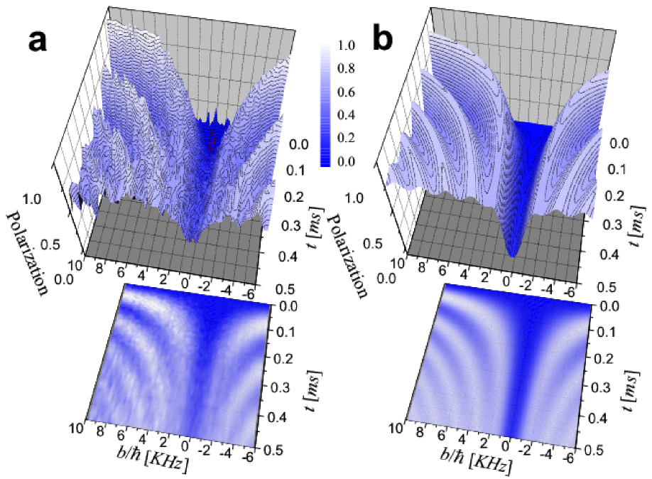
Figure 1: (Color online) Spin swapping dynamics in ¹³C-¹H. (a): Experimental ¹³C polarization in Fe(C₅H₅)₂ as a function of the contact time $t$ and spin-spin coupling $b(\theta)$. (b): Numerical simulations of the ¹³C polarization obtained from Eq. (7) for different values of $b$, a dipolar system-environment interaction $\left(\left|\alpha/\beta\right|=2\right)$ and a constant value for $\tau_{\mathrm{SE}}$ ($\tau_{\mathrm{SE}}=0.275~{}\mathrm{ms}$) obtained by fitting the experimental data in the regime where the MKBE expression is valid. Projection plots in the $b-t$ plane show a canyon where the oscillation period diverges indicating a Quantum Dynamical Phase Transition.

A noticeable feature in these experimental data is the presence of a “canyon”, in the region $\left|b\right|<2~{}$kHz, where oscillations (swapping) disappear. The white hyperbolic stripes in the contour plot at the bottom evidence a swapping period $2\pi/\omega$ that diverges for a non-zero critical interaction. This divergence is the signature of a critical behavior.

The standard procedure to characterize the cross polarization experiment in ferrocene and similar compoundsJCP98 is derived from the MKBE model. There the ¹³C polarization exchanges with that of its directly bonded ¹H, which, in turn, interacts isotropically with other protons that constitute the environment.MKBE Their solution is

$$P^{{}^{\mathrm{MKBE}}}(t)=1-\frac{1}{2}\exp\left[-\frac{t}{2\tau_{\phi}}\right]-\frac{1}{2}\cos(\omega t)\exp\left[-\frac{3}{2}\frac{t}{2\tau_{\phi}}\right]),$$ (2)

where the decoherence rate becomes determined by the rate of interaction with the environment $1/\left(2\tau_{\mathrm{SE}}\right)\rightarrow 1/\left(2\tau_{\phi}\right)\equiv R,$ while the swapping frequency is given by the two-spin dipolar interaction, $b/\hbar\rightarrow\omega$. A dependence of the inputs $b$ and $\tau_{\mathrm{SE}}$ on $\theta$ should manifest in the observables $\omega$ and $\tau_{\phi}.$ However, working on a polycrystal, each $\tau_{\mathrm{SE}}(\theta)$ value involves a cone of orientations of neighboring molecules and a rough description with single average value for the SE interaction rate is suitable.

We have performed non-linear least square fittings of the experimental points to the equation $P^{{}^{\mathrm{MKBE}}}(t)$ for the whole ¹³C spectra of ferrocene in steps of $\approx 80\mathrm{Hz}$ and contact times ranging from $2\mathrm{\mu s}$ to $3\mathrm{ms}$. The $1/\left(2\tau_{\phi}\right)$ and $\omega$ parameters obtained from these fits are shown as dots in Fig. 2. The proportionality of the frequency with $b$ for orientations that are far from the magic angle is verified. In this region a weak variation of $1/\left(2\tau_{\phi}\right)$ around $2.2\mathrm{kHz}$ reflects the fact that $1/\left(2\tau_{\mathrm{SE}}\right)$ does not depend on $\theta$. A drawback of this simple characterization is that it tends to overestimate the width of the canyon because of limitations of the fitting procedure when Eq. (2) is used around the magic angle.

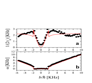
Figure 2: (Color online) Decoherence rate 1/(2$\tau_{\phi}$) and frequency $\omega$ in the spin swapping of a ¹³C-¹H system. Data points are obtained by fitting cross polarization experiments to the expression $P^{{}^{\mathrm{MKBE}}}(t)$. The zero plateau in the frequency and the parabolic behavior of $1/(2\tau_{\phi})$ in the region $b\tau_{\mathrm{SE}}\ll\hbar$ are indicative of an over-damped Zeno phase. Solid lines are the prediction of our model assuming a constant $\tau_{\mathrm{SE}}=0.275\ ms$.

In spite of the MKBE theoretical prediction, one observes that the frequency becomes zero abruptly and the relaxation rate suddenly drops with a quadratic behavior when $b_{\mathrm{c}}\simeq 2\mathrm{kHz}$. The minimum of the parabola occurs at the magic angle, when $b=0.$ Then, all the polarization reaching the ¹³C at this orientation originates from protons outside the molecule. Then, the rate of $0.5\mathrm{kHz}$ obtained at this minimum constitutes an experimental estimation of this mechanism. This has to be compared with the almost constant value of $1/(2\tau_{\mathrm{SE}})=1/(2\tau_{\phi})\simeq$ $2.2\mathrm{kHz}$ observed outside the magic angle neighborhood. This justifies neglecting the J-coupling and the direct relaxation of the ¹³C polarization through the dipolar interaction with protons outside the molecule. In the following we describe our stroboscopic model that accounts for the “anomalous” experimental behavior.

III THEORETICAL DESCRIPTION

III.1 The system

Let us consider $M$ coupled $1/2$ spins with a Hamiltonian:

$$\mathcal{H}=\mathcal{H}_{\mathrm{Z}}+{\textstyle\sum\limits_{i<j}}\left[a_{ij}I_{i}^{z}I_{j}^{z}+b_{ij}\left(I_{i}^{+}I_{j}^{-}+I_{i}^{-}I_{j}^{+}\right)/2\right],$$ (3)

where $\mathcal{H}_{\mathrm{Z}}=\sum_{i=1}^{M}\hbar\left(\omega_{\mathrm{L}}+\delta\omega_{i}\right)I_{i}^{z}$ is the Zeeman energy, with a mean Larmor frequency $\omega_{\mathrm{L}}$. The second term is the spin-spin interaction: $b_{ij}/a_{ij}=0$ is Ising, and $a_{ij}/b_{ij}=0,1,-2$ gives an $XY$, an isotropic (Heisenberg) or the truncated dipolar (secular), respectively. This last case is typical in solid-state NMR experiments QME where $\hbar\delta\omega_{i},a_{ij},b_{ij}\ll\hbar\omega_{\mathrm{L}}$.

In order to describe the experimental system let us take the first $N=2$ spins, $I_{1}$ (a ¹³C) and $I_{2}$ (its directly bonded ¹H), as the “system” where the swapping $\left|\downarrow_{1}\uparrow_{2}\right\rangle\rightleftarrows\left|\uparrow_{1}\downarrow_{2}\right\rangle$ occurs under the action of $b_{12}$. The other $M-N$ spins (all the other ¹H), with $M\rightarrow\infty$, are the spin-bath or “environment”. This limit enables the application of the Fermi Golden Rule or a more sophisticated procedure to obtain a meanlife $\tau_{\mathrm{SE}}$ for the system levels. We will not need much detail for the parameters of the spin bath in Eq. (3) except for stating that it is characterized by an energy scale $d_{\mathrm{B}}$ which leads to a very short correlation time $\tau_{\mathrm{B}}\simeq\hbar/d_{\mathrm{B}}$.

III.2 Spin$\leftrightarrow$Fermion mapping

The spin system can be mapped into a fermion particle system using the Jordan-Wigner transformation,spin-fermion ; spin-fermion2 $I_{i}^{+}=c_{i}^{+}\exp\left\{\mathrm{i}\pi\sum_{j=1}^{i-1}c_{j}^{+}c_{j}\right\}$. Under the experimental conditions, $\delta\omega_{i}=0,$ $a_{12}=0$ and $b_{12}=b,$ the system Hamiltonian becomes:

$$\mathcal{H}_{\mathrm{S}}=\hbar\omega_{\mathrm{L}}\left(c_{1}^{+}c_{1}+c_{2}^{+}c_{2}-\mathbf{1}\right)+b\left(c_{1}^{+}c_{2}+c_{2}^{+}c_{1}\right)/2.$$ (4)

The Jordan-Wigner transformation maps a linear many-body $XY$ spin Hamiltonian into a system of non-interacting fermions. This leads us to solve a one-body problem, reducing the dimension of the Hilbert space from $2^{N}$ to $N$ states that represent local excitations.spin-fermion ; spin-fermion2 To simplify the presentation, and without loss of generality, we consider a single connection between the system and the spin bath, $a_{23}=\alpha d_{23}$ and $b_{23}=\beta d_{23}$ with $a_{2j}=b_{2j}=0,$ $j=4\ldots\infty$ and $a_{1j}=b_{1j}=0,$ $j=3\ldots\infty$. Spins $I_{i}$ with $3\leq i\leq M$ are interacting among them. The SE interaction becomes:

$$\mathcal{V}=d_{23}\left[\alpha\left(c_{2}^{+}c_{2}-\tfrac{1}{2}\right)\left(c_{3}^{+}c_{3}-\tfrac{1}{2}\right)+\beta\left(c_{2}^{+}c_{3}+c_{3}^{+}c_{2}\right)/2\right].$$ (5)

In the first (Ising) term, the first factor “measures” if there is a particle at site $2$ while the second “measures” at site$\ 3$. Hence, polarization at site $2$ is “detected” by the environment. The hopping term swaps particles between bath and system.

In the experimental initial condition, all spins are polarized with the exception of $I_{1}$.MKBE ; JCP2003 In the high temperature limit ($\hbar\omega_{\mathrm{L}}/k_{B}T\equiv s\ll 1$), the reduced density operator is $\mathbf{\sigma}\left(0\right)=\frac{\hbar}{\mathrm{i}}\mathbf{G}^{<}\left(0\right)=\left(\mathbf{1}+sI_{2}^{z}\right)/\operatorname{Tr}\left\{\mathbf{1}\right\}$ which under the Jordan-Wigner transformation becomes $\frac{\left(1-s/2\right)}{\operatorname{Tr}\left\{\mathbf{1}\right\}}\mathbf{1}+\frac{s}{\operatorname{Tr}\left\{\mathbf{1}\right\}}c_{2}^{+}c_{2}.$ Since the first term does not contribute to the dynamics, we retain only the second term and normalize it to the occupation factor. This means that site $1$ is empty while site $2$ and sites at the particle reservoir are “full”. This describes the tiny excess above the mean occupation $1/2.$ To find the dynamics of the reduced density matrix of the “system” $\mathbf{\sigma}\left(t\right)=\frac{\hbar}{\mathrm{i}}\mathbf{G}^{<}\left(t\right),$ we will take advantage of the particle representation and use an integral form Keldysh ; Keldysh2 of the Keldysh formalism instead of the standard Liouville-von Neumann differential equation. There, any perturbation term is accounted to infinite order ensuring the proper density normalization. The interaction with the bath is local and, because of the fast dynamics in the bath, it can be taken as instantaneous. Hence, the evolution is further simplified into an integral form of the Generalized Landauer Büttiker Equation (GLBE) GLBE1 ; GLBE2 for the particle density. There, the environment plays the role of a local measurement apparatus. Firstly, we discuss the physics in this GLBE by developing a discrete time version where the measurements occur at a stroboscopic time $\tau_{\mathrm{str.}}$.

III.3 Stroboscopic Decoherent Model

We introduce our computational procedure operationally for an Ising form ($\beta/\alpha=0$) of $\mathcal{V}$. The initial state of the isolated two-spin system evolves with $\mathcal{H}_{\mathrm{S}}$. At $\tau_{\mathrm{str.}}$, the spin bath interacts instantaneously with the “system” interrupting it with a probability $p$. The actual physical time for the SE interaction is then obtained as $\tau_{\mathrm{SE}}=\tau_{\mathrm{str.}}/p$. Considering that the dynamical time scale of the bath ($\tau_{\mathrm{B}}\simeq\hbar/d_{\mathrm{B}}$) is much faster than that of the system (fast fluctuation approximation), the dynamics of site $3$ produces an energy fluctuation on site $2$ that destroys the coherence of the two-spin “system”. This represents the “measurement” process that collapses the “system” state. At time $\tau_{\mathrm{str.}}$, the “system” evolution splits into three alternatives: with probability $1-p$ the state survives the interruption and continues its undisturbed evolution, while with probability $p$ the system is effectively interrupted and its evolution starts again from each of the two eigenstates of $c_{2}^{+}c_{2}$. These three possible states at $\tau_{\mathrm{str.}}$ evolve freely until the system is monitored again at time $2\tau_{\mathrm{str.}}$ and a new branching of alternatives is produced as represented in the scheme of Fig. 3a.

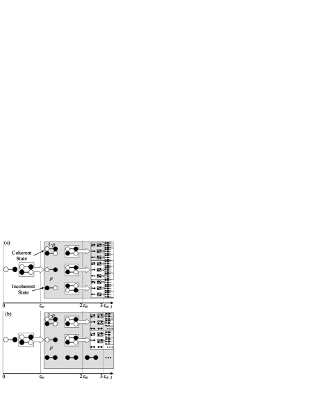
Figure 3: Quantum branching sequence for the swapping dynamics. Panel (a) stands for an Ising system-environment interaction and (b) an isotropic one. Single states represent states with interrupted evolution (incoherent) while pairs of states are coherent superpositions. Notice the self-similar structure.

A similar reasoning holds when $\beta\neq 0.$ The sequence for isotropic interaction ($\alpha=\beta$) is shown in Fig. 3b. The $XY$ part of $\mathcal{V}$  can inject a particle. When an interruption occurs, the bath “measures” at site $2$ and, if found empty, it injects a particle. In the figure, this can be interpreted as a “pruning” of some incoherent branches increasing the global coherence. This explains why the rate of decoherence is greater when the Ising part of $\mathcal{V}$ dominates over the $XY$ part. This occurs with the dipolar interaction and, in less degree, with the isotropic one. This contrasts with a pure $XY$ interaction where the survival of spin coherences is manifested by a “spin wave” behavior.Madi1997 The empty site of the bath is refilled and de-correlates in a time much shorter than the swapping between sites $1$ and $2$ (fast fluctuation approximation). Consequently, the injection can only occur from the bath toward the system.

III.4 Analytical solution

The free evolution between interruptions is governed by the system’s propagators $\mathbf{U}_{\mathrm{S}}\left(t\right)=\exp[-\mathrm{i}\mathcal{H}_{\mathrm{S}}t/\hbar]=-\frac{\hbar}{\mathrm{i}}\mathbf{G}^{0\mathrm{R}}\left(t\right)$. The spin bath interacts with the system stroboscopically through an instantaneous interruption function $\widetilde{\mathbf{\Sigma}}^{<}\left(t\right)=\frac{1}{\mathrm{i}\hbar}\frac{\tau_{\mathrm{str.}}}{p}\mathbf{\Sigma}^{<}\left(t\right)$. The reduced density function is

$$\mathbf{\sigma}\left(t\right)=\mathbf{U}_{\mathrm{S}}\left(t\right)\mathbf{\sigma}\left(0\right)\mathbf{U}_{\mathrm{S}}^{{\dagger}}\left(t\right)\left(1-p\right)^{n}+$$ (6)

$${\textstyle\sum\limits_{m=1}^{n}}\mathbf{U}_{\mathrm{S}}\left(t-t_{m}\right)\widetilde{\mathbf{\Sigma}}^{<}\left(t_{m}\right)\mathbf{U}_{\mathrm{S}}^{{\dagger}}\left(t-t_{m}\right)p\left(1-p\right)^{n-m},$$

where $n=\operatorname{int}\left(t/\tau_{\mathrm{str.}}\right)$ is the number of interruptions and $t_{m}=m\tau_{\mathrm{str.}}$. The first term in the rhs is the coherent system evolution weighted by its survival probability $\left(1-p\right)^{n}.$ This is the upper branch in Fig. 3. The second term is the incoherent evolution involving all the decoherent branches. The $m$-th term in the sum represents the evolution that had its last interruption at $m\tau_{\mathrm{str.}}$ and survived coherently from $m\tau_{\mathrm{str.}}$ to $n\tau_{\mathrm{str.}}$. Each of these is composed by all the interrupted branches in Fig. 3 with a single state at the hierarchy level $m$ with whom the paired state in the upper branch, generated at time $\left(m+1\right)\tau_{\mathrm{str.}},$ keeps coherence up to $n\tau_{\mathrm{str.}}$.

In a continuous time process ($\tau_{\mathrm{SE}}=\tau_{\mathrm{str.}}/p$ with $p\rightarrow 0$ and $\tau_{\mathrm{str.}}\rightarrow 0$), the above procedure gives a physical meaning for the Keldysh’s self-energy GLBE1 ; GLBE2 as an instantaneous interruption function: $\mathbf{\Sigma}^{<}\left(t\right)=\mathbf{\Sigma}_{\mathrm{m}}^{<}\left(t\right)+\mathbf{\Sigma}_{\mathrm{i}}^{<}\left(t\right)$ (see appendix). Dissipation processes are in $\mathbf{\Sigma}_{\mathrm{i}}^{<}\left(t\right)$ while $\mathbf{\Sigma}_{\mathrm{m}}^{<}\left(t\right)$ involves only decoherence. The term $\mathbf{\Sigma}_{\mathrm{i}}^{<}\left(t\right)$ injects a particle, increasing the system density, provided that site $2$ is empty. This occurs at an injection rate $p_{\mathrm{XY}}/\tau_{\mathrm{SE}}=\Gamma_{\mathrm{XY}}/\hbar$ with $p_{\mathrm{XY}}=\left[\beta^{2}/\left(\alpha^{2}+\beta^{2}\right)\right],$ the $XY$ interaction weight. The decoherent part, $\mathbf{\Sigma}_{\mathrm{m}}^{<}\left(t\right),$ is a consequence of the “measurement” (or interruption) performed by the environment. It collapses the state vanishing the non-diagonal terms (coherences) with a measurement rate $\Gamma_{\mathrm{ZZ}}/\hbar=\left(1-p_{\mathrm{XY}}\right)/\tau_{\mathrm{SE}}.$ This also occurs with the $XY$ interaction with rate $\Gamma_{\mathrm{XY}}/\hbar$ regardless of the fact that an effective injection takes place. Then, the inverse of the survival time or interruption rate is $\hbar/\tau_{\mathrm{SE}}=\Gamma_{\mathrm{SE}}=\Gamma_{\mathrm{ZZ}}+\Gamma_{\mathrm{XY}}$. Unlike $\mathbf{\Sigma}_{\mathrm{i}}^{<}\left(t\right)$, this process conserves the total polarization. We denote by $\Gamma/\hbar$ the rate associated to the isotropic interaction ($\alpha=\beta=1$). Then, the anisotropic rates are: $\Gamma_{\mathrm{ZZ}}=\alpha^{2}\Gamma$ and $\Gamma_{\mathrm{XY}}=\beta^{2}\Gamma,$ then $\hbar/\tau_{\mathrm{SE}}=\Gamma_{\mathrm{SE}}=\left(\alpha^{2}+\beta^{2}\right)\Gamma$. The rates can be calculated to infinite order in perturbation theory from the solution of the bath dynamics in a chain of spins with $XY$ interactions,condmat2004 which in the limit $d_{23}/d_{\mathrm{B}}\rightarrow 0$ gives $\Gamma_{\mathrm{XY}}=2\pi\beta^{2}d_{23}^{2}(\pi d_{\mathrm{B}})^{-1}=\beta^{2}\Gamma$ which recovers a Fermi golden rule evaluation.

The anisotropy ratio $\left(\alpha/\beta\right)^{2}$ accounts for the observed competition JCP2003 between the Ising and $XY$ terms of $\mathcal{V}$. The Ising interaction drives the “system” to the internal quasi-equilibrium. In contrast, the $XY$ term allows the thermal equilibration with the bath.JCP2003 Solving Eq. (6) in the limit of continuos time processes we obtain our main analytical result for the swapping probability (experimental ¹³C polarization):

$$P\left(t\right)=1-a_{0}e^{-R_{0}t}-a_{1}\cos\left[\left(\omega+\mathrm{i}R_{2}\right)t+\phi_{0}\right]e^{-R_{1}t},$$ (7)

which, in spite of appearance, has a single fitting parameter. This is because the real functions $\omega,$ $R_{0},R_{1}$ and $R_{2}$ as well as $a_{0}$, $a_{1}$ and $\phi_{0}$ depend exclusively on $b,$ $\tau_{\mathrm{SE}}$ and $p_{\mathrm{XY}}$. Besides, $b$ and $p_{\mathrm{XY}}$ are determined from crystallography and the anisotropy of the magnetic interaction ($p_{\mathrm{XY}}=1/5$ for dipolar) respectively. The phase transition is ensured by the condition $\omega R_{2}\equiv 0$. The complete analytical expression is given in the appendix.

III.5 Limiting cases

Typical solutions of the quantum master equation QME for a spin swapping JCP2003 follow that of MKBE MKBE . They considered an isotropic interaction with the spin environment, represented by a phenomenological relaxation rate $1/\left(2\tau_{\mathrm{SE}}\right).$ Within the fast fluctuation approximation and neglecting non-secular terms, this leads to $P^{{}^{\mathrm{MKBE}}}\left(t\right),$ used in most of the experimental fittings. Our Eq. (7) reproduces this result with $1/\left(2\tau_{\phi}\right)\equiv R\simeq 1/\left(2\tau_{\mathrm{SE}}\right)$ by considering an isotropic interaction Hamiltonian $\alpha=\beta=1$ under the condition $1/\left(2\tau_{\mathrm{SE}}\right)\ll b/\hbar.$ However, at short times $t\ll\tau_{\mathrm{SE}},$ the MKBE swapping probability growths exponentially with a rate $1/\left(2\tau_{\mathrm{SE}}\right)$. In contrast, our solution manifests the quadratic polarization growth in time, $\left(\frac{1}{2}b/\hbar\right)^{2}t^{2}.$ In Eq. (7) this is made possible by the phase $\phi_{0}$ in the cosine. In the opposite parametric region, $b\tau_{\mathrm{SE}}\ll\hbar$,  our model enables the manifestation of the quantum Zeno effect.Usaj ; Misra ; PascazioQZSub2002 This means that the bath interrupts the system through measurements too frequently, freezing its evolution. At longer times, $t\gg\tau_{\mathrm{SE}}$, one gets $1-P\left(t\right)\sim\left(1+\frac{1}{2}\left(b/\hbar\right)^{2}\tau_{\mathrm{SE}}^{2}\right)\exp\left[-\frac{1}{2}(b/\hbar)^{2}\tau_{\mathrm{SE}}t\right],$ and the quantum Zeno effect is manifested in the reduction of the decay rate $1/\left(2\tau_{\phi}\right)\propto\left(b/\hbar\right)^{2}\tau_{\mathrm{SE}}$ as $\tau_{\mathrm{SE}}$ gets smaller than $\hbar/b$. This surprising dependence deserves some interpretation. First, we notice that a strong interaction with the bath makes the ¹H spin to fluctuate, according to the Fermi golden rule, at a rate $1/\tau_{\mathrm{SE}}$. The effect on the ¹³C is again estimated in a fast fluctuation approximation as $1/\tau_{\phi}\propto\left(b/\hbar\right)^{2}\tau_{\mathrm{SE}}$ $\propto\left(b/\hbar\right)^{2}\left[\left(d_{23}/\hbar\right)^{2}\tau_{\mathrm{B}}\right]^{-1}$. This “nesting” of two Fermi golden rule rates is formally obtained from a continued fractions evaluation of the self-energies DAmato ; condmat2004 involving an infinite order perturbation theory. Another relevant result is that the frequency depends not only on $b$, but also on $\tau_{\mathrm{SE}}.$ A remarkable difference between the quantum master equation and our formulation concerns the final state. In the quantum master equation $\sigma\left(\infty\right)$ must be hinted beforehand, while here it is reached dynamically from the interaction with the spin bath. Here, the reduced density, whose trace gives the system polarization, can fluctuate until it reaches its equilibrium value.

III.6 Comparison with the experiments

In order to see how well our model reproduces the experimental behavior we plot the ¹³C polarization with realistic parameters. Since the system is dominated by the dipolar SE interaction,JCP2003 we take $\left|\alpha/\beta\right|=2.$ We introduce $b$ with its angular dependence according to Eq. (1) and we select a constant value for $\tau_{\mathrm{SE}}=0.275~{}\mathrm{ms}$ representative of the $b\gg\hbar/\tau_{\mathrm{SE}}$ regime. Since in this work, we are only interested in the qualitative aspects of the critical behavior of the dynamics, there is no need to introduce $\tau_{\mathrm{SE}}(\theta)$ as a fitting parameter. These evolutions are normalized at the maximum contact time ($3\ \mathrm{ms}$) experimentally acquired. They are shown in Fig. 1b where the qualitative agreement with the experimental observation of a canyon is evident. Notice that the experimental canyon is less deep than the theoretical one. This is due to intermolecular ¹³C-¹H couplings neglected in the model. We will show that the analytical expression of Eq. (7) allows one to determine the edges of the canyon which are the critical points of what we will call a Quantum Dynamical Phase Transition.

IV QUANTUM DYNAMICAL PHASE TRANSITION

Our quantum observable (the local spin polarization) is a binary random variable. The dynamics of its ensemble average (swapping probability), as described by Eq. (7), depends parametrically on the “noisy” fluctuations of the environment through $\tau_{\mathrm{SE}}$. Thus, following Horsthemke and Lefever,Horsthemke-Lefever one can identify the precise value for $\tau_{\mathrm{SE}}$ where a qualitative change in the functional form of this probability occurs as the critical point of a phase transition. This is evidenced by the functional change (nonanalyticity) of the dependence of the observables (e.g. the swapping frequency $\omega$) on the control parameter $b\tau_{\mathrm{SE}}/\hbar$. Since the control parameter switches among dynamical regimes we call this phenomenon a Quantum Dynamical Phase Transition.

It should be remarked that the effect of other spins on the two spin system introduces non-commuting perturbing operators (symmetry breaking perturbations) which produce non-linear dependences of the observables. While this could account for the limiting dynamical regimes, it does not ensure a phase transition. A true phase transition needs a non-analyticity in these functions which is only enabled by taking the thermodynamic limit of an infinite number of spins.sachdev In our formalism, this is incorporated through the imaginary part of the energy, $\hbar/\tau_{\mathrm{SE}},$ evaluated from the Fermi Golden Rule.condmat2004

When the SE interaction is anisotropic ($\alpha\neq\beta$), there is a functional dependence of $\omega\$on $\tau_{\mathrm{SE}}$ and $b$ yielding a critical value for their product, $b\tau_{\mathrm{SE}}/\hbar=k_{p_{\mathrm{XY}}},$ where the dynamical regime switches. One identifies two parametric regimes: 1- The swapping phase, which is a form of sub-damped dynamics, when $b\tau_{\mathrm{SE}}/k_{p_{\mathrm{XY}}}>\hbar$ ($R_{2}=0$ in Eq. (7)). 2- A Zeno phase, with an over-damped dynamics for $b\tau_{\mathrm{SE}}/k_{p_{\mathrm{XY}}}<\hbar$ as a consequence of the strong coupling with the environment (zero frequency, i.e. $\omega=0$, in Eq. (7)). In the neighborhood of the critical point the swapping frequency takes the form (see appendix):

$$\omega=\left\{\begin{array}[c]{cc}a_{p_{\mathrm{XY}}}\sqrt{\left(b/\hbar\right)^{2}-k_{p_{\mathrm{XY}}}^{2}/\tau_{\mathrm{SE}}^{2}}&b\tau_{\mathrm{SE}}/k_{p_{\mathrm{XY}}}>\hbar\\ 0&b\tau_{\mathrm{SE}}/k_{p_{\mathrm{XY}}}\leq\hbar\end{array}\right..$$ (8)

The parameters $a_{p_{\mathrm{XY}}}$ and $k_{p_{\mathrm{XY}}}$ only depend on $p_{\mathrm{XY}}$ which is determined by the origin of the interaction Hamiltonian. For typical interaction Hamiltonians the values of these parameters $\left(p_{\mathrm{XY}},k_{p_{\mathrm{XY}}},a_{p_{\mathrm{XY}}}\right)$ are: Ising $\left(0,\frac{1}{2},1\right)$, dipolar $\left(\frac{1}{5},0.3564,0.8755\right)$, isotropic $\left(\frac{1}{2},0,\frac{1}{\sqrt{2}}\right)$ and $XY$ $\left(1,1,1\right).$ The swapping period is

$$T\simeq\frac{T_{0\mathrm{c}}^{3/2}}{\sqrt{2}a_{p_{\mathrm{XY}}}}\ \left(T_{0\mathrm{c}}-T_{0}\right)^{-1/2},$$ (9)

where $T_{0}=\frac{2\pi\hbar}{b}$ is the isolated two spin period and its critical value $T_{0\mathrm{c}}=\frac{2\pi\tau_{\mathrm{SE}}}{k_{p_{\mathrm{XY}}}},$ determines the region where the period $T$ diverges as is observed in Fig. 1.  The estimated value of $\tau_{\mathrm{SE}}=0.275~{}\mathrm{ms}$ and dipolar SE interactions yield a critical value for the ¹³C-¹H coupling of $b_{\mathrm{c}}/\hbar=2\pi/T_{0\mathrm{c}}=1.3~{}\mathrm{kHz.}$

The complete phase diagram that accounts for the anisotropy of the SE interactions is shown in Fig. 4. There, the frequency dependence on $p_{\mathrm{XY}}$ and $b\tau_{\mathrm{SE}}/\hbar$ is displayed. At the critical line the frequency becomes zero setting the limits between both dynamical phases.

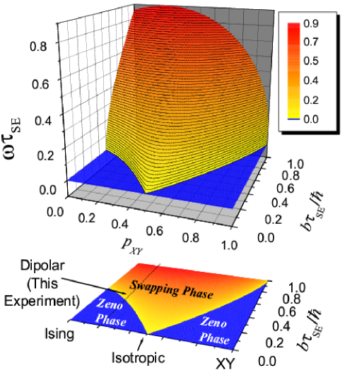
Figure 4: (Color online) Quantum dynamical phase diagram for the spin swapping operation. The figure shows the frequency dependence on system-environment (SE) interaction anisotropy $p_{\mathrm{XY}}$ and the ratio among the internal and the SE interaction $b\tau_{\mathrm{SE}}/\hbar$. The projection over the $b\tau_{\mathrm{SE}}/\hbar-p_{\mathrm{XY}}$ plane determines the phase diagram where the transition between the swapping phase into the Zeno phase ($\omega=0)$ is manifested. Values of $p_{\mathrm{XY}}$ for typical SE interaction Hamiltonian are indicated in the contour plot.

The two dynamical phases can now be identified in the NMR experiments which up to date defied explanation. The experimental setup provides a full scan of the parameter $b\tau_{\mathrm{SE}}$ through the phase transition that is manifested when the frequency goes suddenly to zero (Fig. 2b) and the relaxation rate (Fig. 2a) changes its behavior decaying abruptly. The fact that $1/\left(2\tau_{\phi}\right)$ tends to zero when $b\ll\hbar/\tau_{\mathrm{SE}}$ confirms the Zeno phase predicted by our model. In this regime, $1/\left(2\tau_{\phi}\right)$ is quadratic on $b$ as prescribed. To make the comparison between the two panels of Fig. 1 quantitative, we fit the predicted dynamics of Fig. 1b with $P^{{}^{\mathrm{MKBE}}}\left(t\right),$ following the same procedure used to fit the experimental data. The solid line in Fig. 2 show the fitting parameters $1/\left(2\tau_{\phi}\right)$ and $\omega$ in excellent agreement with the experimental ones.

We point out that Eq. (2) is used to fit both the experiments and the theoretical prediction of Eq. (7) because it constitutes a simple, thought imperfect, way to extract the “outputs” (oscillation frequency $\omega$ and a decoherence time $\tau_{\phi}$). While the systematic errors shift the actual critical value of the control parameter, $b/\hbar$, from $1.3~{}\mathrm{kHz}$ to $2~{}\mathrm{kHz}$, Eq. (2) yields a simplified way to “observe” the transition.

V CONCLUSIONS

We found experimental evidence that environmental interactions can drive a swapping gate through a Quantum Dynamical Phase Transition towards an over-damped or Zeno phase. The NMR experiments in spin swapping in a ¹³C-¹H system enable the identification and characterization of this phase transition as function of the ratio $b\tau_{\mathrm{SE}}/\hbar$ between the internal and SE interaction. We developed a model that describes both phases and the critical region with great detail, showing that it depends only on the nature of the interaction. In particular the phase transition does not occurs if the SE interaction is restricted to isotropic spin coupling. The phase transition is manifested not only in the observable swapping frequency but also in the decoherence rate $1/\tau_{\phi}$. While a standard Fermi golden rule perturbative estimation would tend to identify this rate with the SE interaction, i.e. $1/\tau_{\phi}\cong 1/\tau_{\mathrm{SE}}$ $\simeq\left(d_{23}/\hbar\right)^{2}\tau_{\mathrm{B}},$ as it occurs well inside the swapping phase, both rates differ substantially as the system enters the Zeno phase ($b\tau_{\mathrm{SE}}\leq k_{p_{\mathrm{XY}}}\hbar$). Here the decoherence rate switches to the behavior $1/\tau_{\phi}\propto\left(b/\hbar\right)^{2}\tau_{\mathrm{SE}}$. In the Zeno phase, the system’s free evolution decays very fast with a rate $\tau_{\mathrm{SE}}^{-1}$. In spite of this, one can see that the initial state as a whole has a slow decay (its dynamics becomes almost frozen) because it is continuously fed by the environment. Since the $\tau_{\mathrm{SE}}$ has become the correlation time for the spin directly coupled to the environment, $1/\tau_{\phi}$ provided by our calculation can be interpreted as a “nested” Fermi golden rule rate emphasizing the non-perturbative nature of the result. Based on the wealth of this simple swapping dynamics, we can foresee applications that range from tailoring the environments for a reduction of their decoherence on a given process to using the observed critical transition in frequency and decoherence rate as a tracer of the environment’s nature. These applications open new opportunities for both, the field of quantum information processing and the general physics and chemistry of open quantum systems.condmat2005

Appendix A

A.1 Discrete time process

It is convenient to rewrite Eq. (6) within the Keldysh formalism where $\mathbf{G}^{<}\left(t\right)=\frac{\mathrm{i}}{\hbar}\mathbf{\sigma}\left(t\right)$ and the evolution operator for the isolated system is $\mathbf{G}^{0\mathrm{R}}\left(t\right)=-\frac{\mathrm{i}}{\hbar}\mathbf{U}_{\mathrm{S}}(t)$, where $\mathbf{G}^{0\mathrm{A}}\left(t\right)=\mathbf{G}^{0\mathrm{R}}\left(t\right)^{{\dagger}}$, and the interruption function $\widetilde{\mathbf{\Sigma}}^{<}\left(t\right)=\frac{1}{\mathrm{i}\hbar}\frac{\tau_{\mathrm{str.}}}{p}\mathbf{\Sigma}^{<}\left(t\right).$ We rearrange expression (6), for $n\tau_{\mathrm{str.}}<t\leq(n+1)\tau_{\mathrm{str.}},$ in terms of $n\tau_{\mathrm{str.}},$ the last interruption time:

$$\tfrac{1}{\hbar^{2}}\mathbf{G}^{<}\left(t\right)=\mathbf{G}^{0\mathrm{R}}\left(t-t_{n}\right)\mathbf{G}^{<}\left(t_{n}\right)\mathbf{G}^{0\mathrm{A}}\left(t-t_{n}\right)\left(1-p\right)$$

$$+\tfrac{\mathrm{i}}{\hbar}\mathbf{G}^{0\mathrm{R}}\left(t-t_{n}\right)\widetilde{\mathbf{\Sigma}}^{<}\left(t_{n}\right)\mathbf{G}^{0\mathrm{A}}\left(t-t_{n}\right)p,$$ (10)

which takes advantage of the self similarity of the hierarchy levels and is simple to iterate. It not only reproduces the results obtained from the quantum theory of continuous irreversible processes GLBE1 ; GLBE2 discussed below, but it provides a very efficient algorithm which reduces memory storage and calculation time substantially.

A.2 Continuous time process

In the limit $p\rightarrow 0$ and $\tau_{\mathrm{str.}}\rightarrow 0$ with constant ratio, one gets a continuous process where $\tau_{\mathrm{SE}}=\tau_{\mathrm{str.}}/p$ defines a survival time for the evolution of the isolated two-spin “system”. Eq. (6) becomes

$$\mathbf{G}^{<}\left(t\right)=\hbar^{2}\mathbf{G}^{0\mathrm{R}}\left(t\right)\mathbf{G}^{<}\left(0\right)\mathbf{G}^{0\mathrm{A}}\left(t\right)e^{-t/\tau_{\mathrm{SE}}}$$

$$+\int_{0}^{t}\mathrm{d}t_{n}\mathbf{G}^{0\mathrm{R}}\left(t-t_{n}\right)\mathbf{\Sigma}^{<}\left(t_{n}\right)\mathbf{G}^{0\mathrm{A}}\left(t-t_{n}\right)e^{-\left(t-t_{n}\right)/\tau_{\mathrm{SE}}},$$ (11)

a new form of the GLBE GLBE1 ; GLBE2 that includes correlations (non-diagonal terms in $\mathbf{G}^{<}$ and $\mathbf{\Sigma}^{<}$). Moreover, keeping $\tau_{\mathrm{SE}}$ constant, under the conditions of finite $\tau_{\mathrm{str.}}\lesssim\hbar/d_{23}$ and $p\lesssim d_{23}/d_{\mathrm{B}}$ (here $d_{\mathrm{B}}$ is a mean intra-bath interaction) there is no significant difference between the stroboscopic approximation and the continuous time description. Thus, the physics of a quantum theory of irreversible processes frerichs91 is obtained by adapting a collapse theory Itano90 into the probabilistic branching scheme represented in Fig. 3. The solutions of Eqs. (6) and (11) are both computationally demanding since they involve a storage of all the previous time steps and reiterated summations. However, Eq. (10) provides a new computation procedure that only requires the information of a single previous step. Besides, it avoids resorting to the random averages required by models that include decoherence through stochastic or kicked-like perturbations.paz2003 ; molmer1992 Thus, it becomes a very practical tool to compute the dynamics in presence of decoherent and dissipation processes.

The instantaneous interruption function: $\mathbf{\Sigma}^{<}\left(t\right)=\mathbf{\Sigma}_{\mathrm{m}}^{<}\left(t\right)+\mathbf{\Sigma}_{\mathrm{i}}^{<}\left(t\right)$ becomes, in matrix form,

$$\mathbf{\Sigma}_{\mathrm{m}}^{<}\left(t\right) =\mathrm{i}\tfrac{\hbar}{\tau_{\mathrm{SE}}}\left(\begin{array}[c]{cc}\tfrac{\hbar}{\mathrm{i}}G_{11}^{<}\left(t\right)&0\\ 0&\tfrac{\hbar}{\mathrm{i}}G_{22}^{<}\left(t\right)\end{array}\right),$$ (14)

$$\mathbf{\Sigma}_{\mathrm{i}}^{<}\left(t\right) =2\mathrm{i}\tfrac{\hbar~{}p_{\mathrm{XY}}}{\tau_{\mathrm{SE}}}\left(\begin{array}[c]{cc}0&0\\ 0&\left[1-\tfrac{\hbar}{\mathrm{i}}G_{22}^{<}\left(t\right)\right]\end{array}\right),$$ (17)

where the physical meaning of the Keldysh’s self-energy GLBE1 ; GLBE2 becomes evident.

Inserting Eq. (14) and (17) in Eq. (11) we obtain our main analytical result, Eq. (7),

$$P\left(t\right) =\tfrac{\hbar}{\mathrm{i}}G_{11}^{<}\left(t\right)$$

$$=1-a_{0}e^{-R_{0}t}-a_{1}\cos\left[\left(\omega+\mathrm{i}R_{2}\right)t+\phi_{0}\right]e^{-R_{1}t},$$ (18)

here all parameters are real with

$$\omega+\mathrm{i}R_{2}=\frac{\sqrt{3}}{2x}\left(\frac{1}{6}\eta\left(p_{\mathrm{XY}},x\right)+6\frac{\phi\left(p_{\mathrm{XY}},x\right)}{\eta\left(p_{\mathrm{XY}},x\right)}\right)b,$$ (19)

where $\omega R_{2}\equiv 0$ and are evaluated with $x=b\tau_{\mathrm{SE}}/\hbar$ using

$$\phi\left(p_{\mathrm{XY}},x\right)=\frac{1}{3}\left(x^{2}-p_{\mathrm{XY}}^{2}-\frac{1}{3}\left(1-p_{\mathrm{XY}}\right)^{2}\right),$$

and

$$\eta\left(p_{\mathrm{XY}},x\right)=\\ \left\{4\left(1-p_{\mathrm{XY}}\right)\left(9x^{2}-2\left(1-p_{\mathrm{XY}}\right)^{2}+18p_{\mathrm{XY}}^{2}\right)\right.\\ \left.+12\left[3\left(4x^{6}-\left(\left(1-p_{\mathrm{XY}}\right)^{2}+12p_{\mathrm{XY}}^{2}\right)x^{4}+\right.\right.\right.\\ \left.\left.\left.4p_{\mathrm{XY}}^{2}\left(5\left(1-p_{\mathrm{XY}}\right)^{2}+3p_{\mathrm{XY}}^{2}\right)x^{2}\right.\right.\right.\\ \left.\left.\left.-4p_{\mathrm{XY}}^{2}\left(\left(1-p_{\mathrm{XY}}\right)^{2}-p_{\mathrm{XY}}^{2}\right)^{2}\right)\right]^{\frac{1}{2}}\right\}^{\frac{1}{3}}.$$

Also,

$$R_{0}=\left(6\frac{\phi\left(p_{\mathrm{XY}},x\right)}{\eta\left(p_{\mathrm{XY}},x\right)}-\frac{1}{6}\eta\left(p_{\mathrm{XY}},x\right)+\right.\\ \left.p_{\mathrm{XY}}+\frac{1}{3}\left(1-p_{\mathrm{XY}}\right)\right)\frac{1}{\tau_{\mathrm{SE}}},$$ (20)

$$R_{1}=\frac{3}{2}\left(p_{\mathrm{XY}}+\frac{1}{3}\left(1-p_{\mathrm{XY}}\right)\right)\frac{1}{\tau_{\mathrm{SE}}}-\frac{R_{0}}{2},$$ (21)

and

$$a_{0} =\frac{1}{2}\frac{2\left(\omega^{2}-R_{2}^{2}\right)+2R_{1}^{2}-b^{2}}{\left(\omega^{2}-R_{2}^{2}\right)+\left(R_{0}-R_{1}\right)^{2}},$$

$$a_{2} =\frac{1}{2\left(\omega+\mathrm{i}R_{2}\right)}\times$$

$$\frac{\left(2R_{0}R_{1}-b^{2}\right)\left(R_{0}-R_{1}\right)+2\left(\omega^{2}-R_{2}^{2}\right)R_{0}}{\left(\omega^{2}-R_{2}^{2}\right)+\left(R_{0}-R_{1}\right)^{2}},$$

$$a_{3} =\frac{1}{2}\frac{b^{2}+2R_{0}^{2}-4R_{0}R_{1}}{\left(\omega^{2}-R_{2}^{2}\right)+\left(R_{0}-R_{1}\right)^{2}},$$

$$a_{1}^{2} =a_{2}^{2}+a_{3}^{2},\;\;\;\;\;\tan\left(\phi_{0}\right)=-\frac{a_{2}}{a_{3}}.$$

The parametric dependence of the swapping frequency $\omega$, Eq. (19), has a critical point at $x=k_{p_{\mathrm{XY}}},$ where the transition occurs. In the neighborhood of this critical point $\omega$ and $R_{2}$ takes the form:

$$\omega=\left\{\begin{array}[c]{cc}a_{p_{\mathrm{XY}}}\sqrt{\left(b/\hbar\right)^{2}-k_{p_{\mathrm{XY}}}^{2}/\tau_{\mathrm{SE}}^{2}}&b\tau_{\mathrm{SE}}/k_{p_{\mathrm{XY}}}>\hbar\\ 0&b\tau_{\mathrm{SE}}/k_{p_{\mathrm{XY}}}\leq\hbar\end{array}\right.,$$ (22)

and

$$R_{2}=\left\{\begin{array}[c]{cc}0&b\tau_{\mathrm{SE}}/k_{p_{\mathrm{XY}}}>\hbar\\ a_{p_{\mathrm{XY}}}\sqrt{k_{p_{\mathrm{XY}}}^{2}/\tau_{\mathrm{SE}}^{2}-\left(b/\hbar\right)^{2}}&b\tau_{\mathrm{SE}}/k_{p_{\mathrm{XY}}}\leq\hbar\end{array}\right.,$$

where

$$k_{p_{\mathrm{XY}}}^{2}=\frac{1}{12}\left\{\left[\left(p_{\mathrm{XY}}-1\right)^{2}\chi\left(p_{\mathrm{XY}}\right)\right]^{\frac{1}{3}}+\zeta\left(p_{\mathrm{XY}}\right)+\right.\\ \left.19p_{\mathrm{XY}}^{2}+\frac{\left(p_{\mathrm{XY}}-1\right)^{\frac{4}{3}}\zeta\left(p_{\mathrm{XY}}\right)}{\left[\chi\left(p_{\mathrm{XY}}\right)\right]^{\frac{1}{3}}}\right\},$$ (23)

$$\chi\left(p_{\mathrm{XY}}\right)=-5291p_{\mathrm{XY}}^{4}-1084p_{\mathrm{XY}}^{3}+546p_{\mathrm{XY}}^{2}-4p_{\mathrm{XY}}+1+\\ 24\sqrt{3}p_{\mathrm{XY}}\sqrt{\left(28p_{\mathrm{XY}}^{2}-2p_{\mathrm{XY}}+1\right)^{3}},$$

$$\zeta\left(p_{\mathrm{XY}}\right)=-215p_{\mathrm{XY}}^{2}-2p_{\mathrm{XY}}+1,$$

and

$$a_{p_{\mathrm{XY}}}^{2}=\frac{1}{2}\frac{\left(f_{1}^{~{}~{}2/3}+36f_{2}\right)\left(-f_{3}f_{1}^{\ \ 2/3}+36f_{2}f_{3}+f_{1}f_{4}\right)}{f_{1}^{~{}~{}5/3}f_{4}},$$ (24)

$$f_{1}=36k_{p_{\mathrm{XY}}}-8+24p_{\mathrm{XY}}+48p_{\mathrm{XY}}^{2}\\ -36k_{p_{\mathrm{XY}}}p_{\mathrm{XY}}-64p_{\mathrm{XY}}^{3}+12f_{4},$$

$$f_{2}=1/3k_{p_{\mathrm{XY}}}-1/3p_{\mathrm{XY}}^{2}-1/9\left(1-p_{\mathrm{XY}}\right)^{2},$$

$$f_{3} =-f_{4}+p_{\mathrm{XY}}f_{4}-6k_{p_{\mathrm{XY}}}-16p_{\mathrm{XY}}^{4}+20p_{\mathrm{XY}}^{3}$$

$$-10p_{\mathrm{XY}}^{2}+13p_{\mathrm{XY}}^{2}k_{p_{\mathrm{XY}}}-2k_{p_{\mathrm{XY}}}p_{\mathrm{XY}}+k_{p_{\mathrm{XY}}},$$

$$f_{4}=\left(12k_{p_{\mathrm{XY}}}+96p_{\mathrm{XY}}^{4}k_{p_{\mathrm{XY}}}-120p_{\mathrm{XY}}^{3}k_{p_{\mathrm{XY}}}+\right.\\ \left.60p_{\mathrm{XY}}^{2}k_{p_{\mathrm{XY}}}-39k_{p_{\mathrm{XY}}}p_{\mathrm{XY}}^{2}+6k_{p_{\mathrm{XY}}}p_{\mathrm{XY}}-3k_{p_{\mathrm{XY}}}\right.\\ \left.-48p_{\mathrm{XY}}^{4}+48p_{\mathrm{XY}}^{3}-12p_{\mathrm{XY}}^{2}\right)^{\frac{1}{2}}.$$

In equation (24) the functions $f_{1},$ $f_{2},$ $f_{3}$ and $f_{4}$ only depend of $p_{\mathrm{XY}}.$

References

- (1) C. H. Bennett and D. P. DiVincenzo, Nature 404, 247 (2000).
- (2) C. J. Myatt et al., Nature 403, 269 (2000).
- (3) D. Vion et al., Science 296, 886 (2002).
- (4) M. Poggio et al., Phys. Rev. Lett. 91, 207602 (2003).
- (5) N. Boulant, K. Edmonds, J. Yang, M. A. Pravia and D. G. Cory, Phys. Rev. A 68, 032305 (2003).
- (6) S. A. Gurvitz, L. Fedichkin, D. Mozyrsky and G. P. Berman, Phys. Rev. Lett. 91, 066801 (2003).
- (7) W. H. Zurek, Rev. Mod. Phys. 75, 715 (2003).
- (8) T. M. Stace and S. D. Barrett, Phys. Rev. Lett. 92, 136802 (2004).
- (9) H. M. Pastawski, P. R. Levstein, G. Usaj, J. Raya and J. A. Hirschinger, Physica A 283, 166 (2000).
- (10) R. A. Jalabert and H. M. Pastawski, Phys. Rev. Lett. 86, 2490 (2001).
- (11) Ph. Jacquod, P. G. Silvestrov and C. W. J. Beenakker, Phys. Rev. E 64, 055203(R) (2001).
- (12) F. M. Cucchietti, H. M. Pastawski and R. A. Jalabert, Phys. Rev. B 70, 035311 (2004).
- (13) Z. L. Mádi, R. Brüschweiller and R. R. Ernst, J. Chem. Phys. 109, 10603 (1998).
- (14) N. Linden, H. Barjat, Ē. Kupče and R. Freeman, Chem. Phys. Lett. 307, 198 (1999).
- (15) L. Müller, A. Kumar, T. Baumann and R. R. Ernst, Phys. Rev. Lett. 32, 1402 (1974).
- (16) A. Abragam, The Principles of Nuclear Magnetism (Clarendon Press, Oxford, 1961).
- (17) P. R. Levstein, G. Usaj and H. M. Pastawski, J. Chem. Phys. 108, 2718 (1998).
- (18) W. Horsthemke and R. Lefever, Noise-Induced Transitions (Springer, Berlin, 1984) Chap. 6 - Sec. 3.
- (19) S. Sachdev, Quantum Phase Transitions (Cambridge U. P., 2001).
- (20) H. M. Pastawski, Phys. Rev. B 44, 6329 (1991), see Eq. 3.7.
- (21) H. M. Pastawski, Phys. Rev. B 46, 4053 (1992), see Eq. 4.11.
- (22) L. V. Keldysh, ZhETF 47, 1515 (1964) [Sov. Phys.-JETP 20, 1018 (1965)].
- (23) P. Danielewicz, Ann. Phys. 152, 239 (1984).
- (24) B. Misra and E. C. G. Sudarshan, J. Math. Phys. 18, 756 (1977).
- (25) H. M. Pastawski and G. Usaj, Phys. Rev. B 57, 5017 (1998).
- (26) P. Facchi and S. Pascazio, Phys. Rev. Lett. 89, 080401 (2002), and references therein.
- (27) C. P. Slichter, Principles of Magnetic Resonance (Springer-Verlag, New York, 1992).
- (28) E. H. Lieb and T. Schultz, D. C. Mattis, Ann. Phys. 16, 407 (1961).
- (29) E. P. Danieli, H. M. Pastawski and P. R. Levstein, Chem. Phys. Lett. 384, 306 (2004).
- (30) A. K. Chattah et al., J. Chem. Phys. 119, 7943 (2003).
- (31) Z. L. Mádi, B. Brutscher, T. Schulte-Herbrüggen, R. Brüschweiler and R. R. Ernst, Chem. Phys. Lett. 268, 300 (1997).
- (32) E. P. Danieli, H. M. Pastawski and G. A. Álvarez, Chem. Phys. Lett. 402, 88 (2005).
- (33) P. R. Levstein, H. M. Pastawski and J. L. D’Amato, J. Phys.: Condens. Matter 2 1781 (1990).
- (34) E. P. Danieli, G. A. Álvarez, P. R. Levstein and H. M. Pastawski, arxiv.org/abs/cond-mat/0511639 predicts a quantum dynamical phase transition in a double quantum dot.
- (35) V. Frerichs and A. Schenzle, Phys. Rev. A 44, 1962 (1991).
- (36) W. M. Itano, D. J. Heinzen, J. J. Bollinger and D. J. Wineland, Phys. Rev. A 41, 2295 (1990).
- (37) G. Teklemariam et al., Phys. Rev. A 67, 062316 (2003).
- (38) J. Dalibard, Y. Castin and K. Mølmer, Phys. Rev. Lett. 68, 580 (1992).