The Dynamics of Hierarchical Evolution of Complex Networks

Abstract

Introduced recently, the concept of hierarchical degree allows a more complete characterization of the topological context of a node in a complex network than the traditional node degree. This article presents analytical characterization and studies of the density of hierarchical degrees in random and scale free networks. The obtained results allowed the identification of a hierarchy-dependent power law for the degrees of nodes in random complex networks, with Poisson density for the first hierarchical degree (obtained through master equation approach). Exact results were obtained for the second hierarchical degree in scale free networks.

I Introduction

The characterization and analysis of complex networks 1 ; 2 involves the use of measurements capable of expressing important properties of the network. While traditional features such as the node degree and clustering coefficient have been successfully used for that purpose, such measurements are intrinsically local, in the sense that they are affected only by the immediate neighborhood of each reference node. Among more global measurements, such as the network diameter and the shortest path between any two network nodes, the concept of hierarchical node degree has been introduced recently and considered for the characterization and analysis of the connectivity of complex networks 4 ; 5 ; 6 ; 7 ; 8 . Given a reference node $i$, it is possible to define the $k-th$ relative hierarchical level as corresponding to the network nodes which are exactly at minimal distance of $k$ edges from node $i$. The hierarchical node degree at level $k$ corresponds to the number of edges between the hierarchical levels $k$ and $k+1$, therefore defining a natural hierarchical extension of the concept of node degree. Note that the hierarchical degree, starting at level $1$ (which includes the immediate neighbors of $i$) tends first to increase with the hierarchical level $k$ and then to decrease as a consequence of the finite size of the network 9 . Because the hierarchical node degree is a global measurement (i.e. it considers, in hierarchical fashion, all nodes in the network), it provides more information about the connectivity of the reference node with the remainder of the network. For instance, the number of hierarchical levels which are required in order to contain a percentage (e.g. 50%) of the network nodes, provides a valuable information about the accessibility of that reference node. The smaller this number of levels, the more connected the reference node is with the rest of the network. Several other topological properties characterizing the context of the reference node can be identified by using the hierarchical node degree and other related features 7 ; 8 .

An interesting question implied by the introduction of the concept of hierarchical node degree regards the analytical characterization of such features expected from random and scale free networks. The current work addresses such an issue by using mean field and the master equation methodologies 3 ; 10 . It is shown that a power law is obtained for the hierarchical degrees of nodes in random networks, with Poisson density being obtained for the first hierarchical degree. We verified that the second order hierarchical degree for scale free networks involves a logarithmic correction of the first order degree studied in 1 ; 2 ; 3 . In addition, we obtain exact results for the second order hierarchical degree distributions in scale free networks.

I.1 Hierarchy and hierarchical degree

A set of hierarchy $h$ is defined as that containing all the vertices which are located at a distance of $h$ connections from a reference vertex. The hierarchical degree, or superior order degree, is the measurement of the number of connections in a set with a determined value of hierarchy. For $h=1$, we have the first order degree which is well known in the literature 1 ; 2 ; 3 . In this article we are intended to study the behavior of graphs where $h\geq 2$. We will denote $k^{(h)}_{i}$ as the degree of order $h$ of the reference vertex $i$; and the set of hierarchy $h$ of the reference vertex $i$ will be denoted as $\{i^{(h)}_{1},i^{(h)}_{2},i^{(h)}_{3},...,i^{(h)}_{k^{(h-1)}_{i}}\}$. We will also denote $N^{(h)}_{x}$ as the number of vertices having hierachical degree $h$ equal to $x$, and $N_{a,b,...,n}$ will denote the number of vertices presenting the first order degree as $a$, the second order degree as $b$ and so on.

II Degree Evolution of a Vertex

Mean field theory is widely applied in complex networks research 1 ; 2 ; 3 . Through this boarding, the degree evolution of the particular vertice is proportional its connection probability (kernel function - $P_{J}(t)$). If this probability has a complex form, the equations become non-trivial.

Generally, the hierarchical degree $h$ depends on the probability of connection of the vertices belonging to this set of hierarchy. Thus, we can write:

$$\frac{\partial k^{(h)}_{j}(t)}{\partial t}=\sum_{i=1}^{k^{(h-1)}_{i}}P_{j^{(h)}_{i}}+\delta_{1h}P_{j}(t)$$ (1)

In the following we consider random graphs where $P_{j}(t)$ is the same for all vertices, as well as scale-free networks proposed by Barabási-Albert 1 where $P_{j}(t)\propto k^{(1)}_{j}$.

III Distribution of the Second Order Connectivity Degree

In this section we will study the connectivity degree distribution, which is an intrinsic characteristic of the complex networks and is capable of distinguishing all types of graphs. Henceforth, for simplicity’s sake, the probability of vertex $j$ to make a connection will be represented as ${\cal P}_{k^{(1)}_{j}}(t)$ and not $P_{j}(t)$.

III.1 Initial States and Structures

A vertex with first order degree $k^{(1)}$ and second order degree $k^{(2)}$ defines one or more structures which are topologically identic and are denoted by $(k^{(1)},k^{(2)})$. For example, Figure 1 shows all possible structures $(3,3)$.

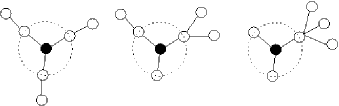
Figure 1: Possible instances of the structure $(3,3)$.

An structure has one or more initial states. An structure $(x_{1},x_{2})$ is the initial state of another structure $(y_{1},y_{2})$ if the following condition is met:

$$(x_{1}+\delta_{1},x_{2}+\delta_{2})\rightarrow(y_{1},y_{2})$$ (2)

where:

$$\delta_{1}+\delta_{2}=1$$ (3)

Therefore, two processes exist which take one structure into the other:

$$(x_{1}+1,y_{2}) \rightarrow (y_{1},y_{2})$$ (4)

$$(y_{1},x_{2}+1) \rightarrow (y_{1},y_{2})$$ (5)

The initial states of structure $(3,3)$, given by $(2,3)$ and $(3,2)$ are represented in Figure 2.

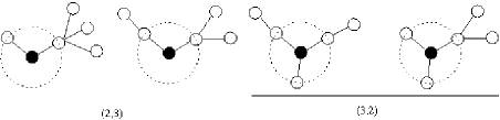
Figure 2: Initial states of structure $(3,3)$.

III.2 Describing the Processes through the Master Equation

The probability of transition of the initial states in a structure give us the production rate of that structure. For example, let us study the formation of structures $(k^{(1)},k^{(2)})$. As we know, their initial states are: $(k^{(1)}-1,k^{(2)})$ and $(k^{(1)},k^{(2)}-1)$. Then, the transition probabilities are given by:

$$P_{(k^{(1)}-1,k^{(2)})\rightarrow(k^{(1)},k^{(2)})} = {\cal P}_{k^{(1)}-1}$$

$$P_{(k^{(1)},k^{(2)}-1)\rightarrow(k^{(1)},k^{(2)})} = {\cal P}_{k^{(1)}+k^{(2)}-1}$$

Therefore, the formation rate of the structure $(k^{(1)},k^{(2)})$ are:

$$N_{+k^{(1)}k^{(2)}} = {\cal P}_{k^{(1)}-1}N_{k^{(1)}-1k^{(2)}}+{\cal P}_{k^{(1)}+k^{(2)}-1}N_{k^{(1)}k^{(2)}-1}$$

$$+ \delta_{1k^{(1)}}{\cal P}_{k^{(2)}}N^{(1)}_{k^{(2)}}$$

The transition probabilities of structure $(k^{(1)},k^{(2)})$ is:

$$P_{(k^{(1)},k^{(2)})\rightarrow(k^{(1)}+1,k^{(2)})} = {\cal P}_{k^{(1)}}$$

$$P_{(k^{(1)},k^{(2)})\rightarrow(k^{(1)},k^{(2)}+1)} = {\cal P}_{k^{(1)}+k^{(2)}}$$

Therefore, the vanishing rate of the structure $(k^{(1)},k^{(2)})$ is:

$$N_{-k^{(1)}k^{(2)}} = [{\cal P}_{k^{(1)}}+{\cal P}_{k^{(1)}+k^{(2)}}]N_{k^{(1)}k^{(2)}}$$

The master equation governing the evolution of $N_{k^{(1)}k^{(2)}}$ is as follows:

$${}\frac{\partial N_{k^{(1)}k^{(2)}}}{\partial t} = {\cal P}_{k^{(1)}-1}N_{k^{(1)}-1k^{(2)}}+{\cal P}_{k^{(1)}+k^{(2)}-1}N_{k^{(1)}k^{(2)}-1}$$ (6)

$$- [{\cal P}_{k^{(1)}}+{\cal P}_{k^{(1)}+k^{(2)}}]N_{k^{(1)}k^{(2)}}$$

$$+ \delta_{1k^{(1)}}{\cal P}_{k^{(2)}}N^{(1)}_{k^{(2)}}$$

In the following we will show the solution of the equation above for random graphs as well as for scale-free networks.

IV Applications

IV.1 Random Graphs

In this work we use non-static version of non-directed random graphs. Instead of generating a network from a symmetric random matrix, we define the following procedure: Beginning with ${\cal N}$ disconnected points, we select two vertices in the network at a time and, with probability $p$, we establish a connection between them. Connections linking a vertex to itself are not allowed, that is to say, the two selected vertices must be different. The probability of a vertex $j$ to be selected at a time $t$ is given by:

$$P_{j}(t)=\frac{p}{{\cal N}}+\frac{p}{{\cal N}-1}=\frac{(2{\cal N}-1)}{{\cal N}({\cal N}-1)}p$$ (7)

IV.1.1 Degree Evolution of a Vertex

Since $P_{j}(t)$ is constant, we will denote it as $\pi$. Therefore:

$$\pi=P_{j}(t)$$ (8)

By substituting Eq.(8) in Eq.(1), we have:

$$\frac{\partial k^{(h)}_{j}(t)}{\partial t}=\pi\left(k^{(h-1)}_{i}+\delta_{1h}\right)$$ (9)

Assuming that $k^{(h)}_{j}=g_{h}t^{h}$, we find $g_{h}=\pi^{h}/h!$ and

$$k^{(h)}_{j}(t) = \frac{(\pi t)^{h}}{h!}$$ (10)

IV.1.2 First Order Degree Distribution

The variation of the number of vertices with first order degree given as $k^{(1)}$ can be described through the master equation:

$$\frac{\partial N^{(1)}_{k^{(1)}}}{\partial t} = \pi[N^{(1)}_{k^{(1)}-1}-N^{(1)}_{k^{(1)}}]$$

As is known, $N^{(1)}_{0}(t=0)={\cal N}$ and $N_{j}(t=0)=0,\forall j$. Solving this equation for $k^{(1)}=0$, we have:

$$N^{(1)}_{0}(t) = {\cal N}e^{-\pi t}$$

And for $k^{(1)}=1$, we have:

$$N^{(1)}_{1}(t) = \pi{\cal N}te^{-\pi t}=\pi tN^{(1)}_{0}(t)$$

For other values of $k^{(1)}$, we conclude that the solution of the master equation obeys the following formation rule:

$$N^{(1)}_{k^{(1)}}(t) = \frac{\pi t}{k^{(1)}}N^{(1)}_{k^{(1)}-1}(t)$$

The solution for this recursion is:

$$N^{(1)}_{k^{(1)}}(t) = {\cal N}\frac{(\pi t)^{k^{(1)}}e^{-\pi t}}{k^{(1)}!}$$

The distribution of the first order degree, given by $P^{(1)}_{k^{(1)}}(t)=N^{(1)}_{k^{(1)}}(t)/{\cal N}$ is:

$$P^{(1)}_{k^{(1)}}(t) = \frac{(\pi t)^{k^{(1)}}e^{-\pi t}}{k^{(1)}!}$$ (11)

This is the Poisson distribution with mean value $\pi t$. Figure 3 shows the time evolution of the number of vertices with $k^{(1)}={0,1,2}$ in a random graph with ${\cal N}=100$ and $p=0.9$.

Figure 3: Evolution of the number of vertices with first order degree $k^{(1)}=\{0,1,2\}$ in a random graph with ${\cal N}=100$ and $p=0.9$.

IV.2 Scale-free Networks

The concept of scale free networks has been introduced by Barabási and Albert and refers to graphs whose first order degree distribution follows a power law 3 : $N_{k^{(1)}}=A[k^{(1)}]^{-\nu}$. Most scale free networks found in nature have $\nu$ in the interval between 2 and 3. The probability of connection in this model is given by:

$$P_{j}(t) = \frac{k^{(1)}_{j}}{\sum_{i=1}^{t}k^{(1)}_{i}}=\frac{k^{(1)}_{j}}{2t}$$ (12)

Also:

$${\cal P}_{k^{(h)}}(t) = \frac{k^{(h-1)}+k^{(h)}}{\sum_{i=1}^{t}k^{(1)}_{i}}=\frac{k^{(h-1)}+k^{(h)}}{2t}$$ (13)

IV.2.1 Evolution of Vertex Degree

Substituting Eq.(12) in Eq.(1), we have:

$$\frac{\partial k^{(h)}_{j}(t)}{\partial t}=\frac{1}{2t}\sum_{i=1}^{k^{(h-1)}_{j}}k^{(1)}_{j^{(h)}_{i}}+\delta_{1h}\frac{k^{(1)}_{j}}{2t}$$ (14)

¿From the definition of hierarchical degree, we have:

$$k^{(h)}_{j}+k^{(h-1)}_{j}=\delta_{1h}k^{(1)}_{j}+\sum_{i=1}^{k^{(h-1)}_{j}}k^{(1)}_{j^{(h)}_{i}}$$ (15)

Therefore:

$$\frac{\partial k^{(h)}_{j}(t)}{\partial t}=\frac{1}{2t}\left(k^{(h)}_{j}+k^{(h-1)}_{j}\right)$$ (16)

For $h=1$ and the following condition: $k^{(1)}_{j}(t=t_{j})=1$ we obtain the solution given by Barabási-Albert in 3 :

$$k^{(1)}_{j}(t)=\sqrt{\frac{t}{t_{j}}}$$ (17)

For $h=2$, we use the integrating factor $t^{-3/2}$ and we obtain:

$$k^{(2)}_{j}(t) = \left[\beta_{2}+\ln{\sqrt{t}}\right]k^{(1)}_{j}(t)$$

If we consider that, in instant where the new vertice is enclosed to network its average second order degree is given by $\kappa^{(2)}_{j}$, then: $k^{(2)}_{j}(t=t_{j})=\kappa^{(2)}_{j}$. From this condition, we have:

$$k^{(2)}_{j}(t) = \left[\kappa^{(2)}_{j}+\ln{k^{(1)}_{j}}\right]k^{(1)}_{j}(t)$$

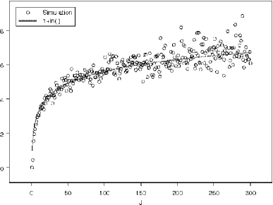
Figure 4: Values of $\kappa^{(2)}_{j}$ in terms of $j$ obtained through numerical simulations are adjusted by the curve $k^{(2)}_{j}=1+\ln{j}$.

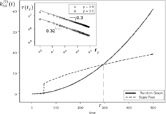
Figure 5: Evolution of $k_{50}^{(2)}(t)$ for a random graph with size ${\cal N}=100$ and connection probability $p=0.9$ and Scale-Free network. The curves intercept at $t=\tau$, indicating that at this growth stage vertex $j$ in the scale free network has the same second order degree as vertex $j$ in the random network. The log-log plot in the inset shows how $\tau(t_{j})$ depends of $t_{j}$, defining power laws $\tau(t_{j})\propto t_{j}^{-\alpha}$. 

Through numerical simulations, we can determine the value of $\kappa^{(2)}_{j}$ in terms of $j$. From Fig(4) we note that $\kappa^{(2)}_{j}=1+\ln{j}$. Thus, the solution for the second order degree variation is given by:

$$k^{(2)}_{j}(t) = \left[1+\ln{t_{j}k^{(1)}_{j}}\right]k^{(1)}_{j}(t)$$ (18)

Eq.(15) is not simple to be solved but, using the same integrating factor as above, we can obtain a solution as an integral recursive equation, as follows:

$$k^{(h)}_{j}(t)=\beta_{h}k^{(1)}_{j}(t)+\frac{1}{2}\sqrt{t}\int{k^{(h-1)}_{j}t^{-\frac{3}{2}}dt}$$ (19)

IV.2.2 First Order Degree Distribution

In 10 , Krapvisky establishes the following master equation which governs the evolution of $N^{(1)}_{k^{(1)}}$, that is, the average number of vertices with first order degree $k^{(1)}$:

$$\frac{\partial N^{(1)}_{k^{(1)}}}{\partial t}=\frac{1}{M(t)}\left[(k^{(1)}-1)N^{(1)}_{k^{(1)}-1}-k^{(1)}N^{(1)}_{k^{(1)}}\right]+\delta_{1k^{(1)}}$$ (20)

The first term takes into account the probability that the new vertex connects to one of the first order degree equal to $k^{(1)}-1$. The second term expresses the probability of connection between a vertex with $k^{(1)}$. The delta function accounts for the fact that every added vertex has degree $1$. By making the normalization $M(t)=2t$, the solution of Eq.(15) is given as:

$$N^{(1)}_{k^{(1)}}(t)=\frac{4t}{k^{(1)}(k^{(1)}+1)(k^{(1)}+2)}$$ (21)

The distribution of the first order degree, i.e. $P^{(1)}_{k^{(1)}}(t)=N^{(1)}_{k^{(1)}}(t)/N_{T}$, is given as:

$$P^{(1)}_{k^{(1)}}(t)=\frac{4}{k^{(1)}(k^{(1)}+1)(k^{(1)}+2)}$$ (22)

Figure 5 shows the evolution of $k_{50}^{(2)}(t)$ for a random graph with $N=100$ nodes and connection probability $p=0.9$ as well as the same measurement for a scale free network. An intersection point can be observed at $t=\tau$, meaning that at this growth stage the vertex $j$ in the random and scale free networks have the same second order degree. For values of $t$ larger than $\tau$, the second order degree becomes larger for the random network than the scale free counterpart. This indicates that the second order degree in a scale free network tends to grow slower than in a random network. The log-log diagram in the inset, shows $\tau(t_{j})$ in terms of $t_{j}$ for connection probabilities $p=0.9$ and $p=0.6$, which yields power laws $\tau(t_{j})\propto t_{j}^{-\alpha}$.

IV.2.3 Second Order Degree Distribution

We now consider the number of vertices with first order degree equal to $k^{(1)}$ and second order degree equal to $k^{(2)}$, which will be represented as $N_{k^{(1)}k^{(2)}}$. The obtention of this quantity involves the solution of Eq.(6). Assuming a linear solution of the type: $N_{k^{(1)}k^{(2)}}=n_{k^{(1)}k^{(2)}}t$, we have:

$$n_{k^{(1)}k^{(2)}} = \frac{{\cal P}_{k^{(1)}-1}n_{k^{(1)}-1k^{(2)}}+{\cal P}_{k^{(1)}+k^{(2)}-1}n_{k^{(1)}k^{(2)}-1}}{{\cal P}_{k^{(1)}}+{\cal P}_{k^{(1)}+k^{(2)}}+1/t}$$

$$+ \frac{\delta_{1k^{(1)}}{\cal P}_{k^{(2)}}n_{k^{(2)}}}{{\cal P}_{1}+{\cal P}_{1+k^{(2)}}+1/t}$$

Substituting Eq.(13) into above expression:

$$n_{k^{(1)}k^{(2)}} = \left[\frac{(k^{(1)}-1)n_{k^{(1)}-1k^{(2)}}}{2k^{(1)}+k^{(2)}+2}\right]$$

$$+ \left(\frac{k^{(1)}+k^{(2)}-1}{2k^{(1)}+k^{(2)}+2}\right)n_{k^{(1)}k^{(2)}-1}$$

$$+ \left(\frac{k^{(2)}n_{k^{(2)}}}{4+k^{(2)}}\right)\delta_{1k^{(1)}}$$

For simplicity’s sake, we make

$$u = k^{(2)}$$ (23)

$$A_{u} = n_{k^{(1)}u}$$ (24)

$$F_{u} = \left[\frac{(k^{(1)}-1)n_{k^{(1)}-1u}}{2k^{(1)}+u+2}\right]+\left(\frac{un_{u}}{4+u}\right)\delta_{1k^{(1)}}$$ (25)

$$G_{u} = \frac{k^{(1)}+u-1}{2k^{(1)}+u+2}$$ (26)

It follows that

$$A_{u}=F_{u}+G_{u}A_{u-1}$$ (27)

In addition, we have to enforce that

$$A_{1}=F_{1},\;\;\;\;\;\;n_{k^{(1)}0}=0$$ (28)

Developing the recurrence, we obtain

$$A_{u} = F_{u}+G_{u}(F_{u-1}+G_{u-1}A_{u-2})$$

$$A_{u} = F_{u}+G_{u}F_{u-1}+G_{u}G_{u-1}(F_{u-2}+G{u-2}A_{u-3})...$$

$$A_{u} = \frac{1}{G_{u+1}}\sum_{f=1}^{u}F_{f}\prod_{g=f}^{u}G_{g+1}$$ (29)

Expressed in terms of the original variables, it follows that

$$n_{k^{(1)}k^{(2)}} = \left(\frac{2k^{(1)}+k^{(2)}+3}{k^{(1)}+k^{(2)}}\right)\sum_{f=1}^{k^{(2)}}\left[\frac{(k^{(1)}-1)n_{k^{(1)}-1f}}{2k^{(1)}+f+2}\right]\prod_{g=f}^{k^{(2)}}\left(\frac{k^{(1)}+g}{2k^{(1)}+g+3}\right)$$

$$+ \frac{\Gamma(k^{(2)}+1)}{\Gamma(k^{(2)}+5)}\sum_{f=1}^{k^{(2)}}f(f+1)(f+2)(f+3)n_{f}$$

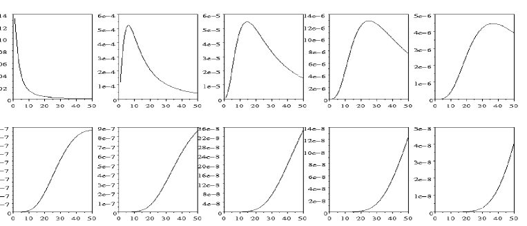
Figure 6: Values of $n_{k^{(1)}k^{(2)}}$ for $k^{(1)}=[1,5,10,15,20,25,30,35,40,45]$ and $k^{(2)}$ in the range 0,50.

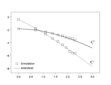
Figure 7: Log-log distribution of $P^{(1)}_{k}$ and $P^{(2)}_{k}$ for Barabási-Albert model of Scale Free Network.

By Eq.(21) we know the value of $n_{f}$ ($n_{f}=N_{f}(t)/t$). Substituting in the above expression:

$$n_{k^{(1)}k^{(2)}}=\left(\frac{2k^{(1)}+k^{(2)}+3}{k^{(1)}+k^{(2)}}\right)\sum_{f=1}^{k^{(2)}}\left[\frac{(k^{(1)}-1)n_{k^{(1)}-1f}}{2k^{(1)}+f+2}\right]\prod_{g=f}^{k^{(2)}}\left(\frac{k^{(1)}+g}{2k^{(1)}+g+3}\right)+\frac{2k^{(2)}(k^{(2)}+7)}{(k^{(2)}+1)(k^{(2)}+2)(k^{(2)}+3)(k^{(2)}+4)}$$ (30)

When $k^{(1)}=1$, we have that

$$n_{1k^{(2)}} = \frac{2k^{(2)}(k^{(2)}+7)}{(k^{(2)}+1)(k^{(2)}+2)(k^{(2)}+3)(k^{(2)}+4)}$$ (31)

This result is identical to the expression obtained by Krapivsky in 10 for correlation degree. Developing the first part of Eq. (30):

$$n_{k^{(1)}k^{(2)}} = n_{1k^{(2)}}+\left(\frac{k^{(1)}-1}{2k^{(1)}+k^{(2)}+2}\right)\sum_{f=0}^{k^{(2)}-1}\left[\frac{\Gamma(2k^{(1)}+f+2)}{\Gamma(k^{(1)}+f)}\right]n_{k^{(1)}-1f}$$ (32)

Figure 6 shows the curves obtained for $n_{k^{(2)}k^{(2)}}$ for several values of $k^{(1)}$ and $k^{(2)}$ varying from 0 to 50.

The total number of vertices with second order degree equal to $k^{(2)}$ is given as:

$$N^{(2)}_{k^{(2)}}(t)=t\sum_{k^{(1)}=1}^{t}n_{k^{(1)}k^{(2)}}$$ (33)

Figure 7 shows a log-log graph of the distribution $N^{(1)}_{k^{(1)}}$ (given by Eq.(21)) and $N^{(2)}_{k^{(2)}}$ (obtained from Eq.(33)). Note that the initial values in this distribution deviate from the linear relation typically observed for scale free networks. The second order distribution, given by $P^{(2)}_{k^{(2)}}(t)=N^{(2)}_{k^{(1)}}(t)/N_{T}$.

V Concluding Remarks

This work addressed the analytical characterization of hierarchical degrees of random and complex networks. In the case of random networks, we have shown that the hierarchical degree follows a power law, i.e. $k^{(h)}(t)\propto t^{h}$. By using the master equation approach, it has also been shown that the first order degree obeys a Poisson distribution. Unlike the first order degree, the evolution of the second order hierarchical degree can not be easily described by a master equation as Eq.(6). This is a consequence of the fact that the adopted approach of uniting two connected components from the network into a single component implies several combinations of effects and respective terms to be incorporated into the master equation. In addition, we verified that the second order degree tends to grow slower in scale free networks than in random networks, with the position where these two values become equal following a power law.

In the case of scale free models, namely the Barabási-Albert network, it has been verified that the second order hierarchical degree, for a particular node, can be expressed in terms of a logarithmic correction of the first order degree. Exact results have been obtained for the second order hierarchical degree. We observe that the generalization of such an approach to higher hierarchical levels becomes substantially more complex because of the need to consider all recursions up to level $h-1$.

Possible continuations of the reported developments include the extension of the analytical expressions of hierarchical node degree to higher levels, as well as the derivation of analytical expression for other hierarchical features such as the hierarchical clustering coefficient and hierarchical number of nodes 4 .

Acknowledgments Luciano da F. Costa thanks HFSP RGP39/2002, FAPESP (proc. 99/12765-2) and CNPq (proc. 3082231/03-1) for financial support.

References

(1)
R. Albert and A.-L. Barabási,
Statistical Mechanics of Complex Networks,
Rev. Mod. Phys. 74, 47 (2002).
(2)
S. N. Dorogovtsev, J. F. F. Mendes and A. N. Samukhin, Structure
of Growing Networks: Exact Solution of the Barabási-Albert’s
Model. cond-mat/0004434.
(3)
A.-L. Barabási, R. Albert and H. Jeong, Mean-Field Theory for
Scale-Free Random Networks, Physica A 272, (1999).
(4)
L. da F. Costa,
The Hierarchical Backbone of Complex Networks,
Phys. Rev. Lett. 93, 098702 (2004).
(5)
L. da F. Costa,
A Generalized Approach to Complex Networks,
cond-mat/0408076.
(6)
L. da F. Costa,
Sznajd Complex Networks,
cond-mat/05001010.
(7)
L. da F. Costa,
Hierarchical Characterization of Complex Networks,
cond-mat/0412761.
(8)
L. da F. Costa,
Scale Free Subnetworks by Design and Dynamics,
cond-mat/0502156.
(9)
R. Pastor-Satorras and A. Vespignani
Epidemic dynamics in finite size scale-free networks,
Phys. Rev. E 65, 035108 (2002).
(10)
P. L. Krapivsky and S. Redner,
Organization of Growing Random Networks,
cond-mat/0011094.