A General Asymptotic Implied Volatility
for Stochastic Volatility Models

Abstract.

In this paper, we derive a general asymptotic implied volatility at the first-order for any stochastic volatility model using the heat kernel expansion on a Riemann manifold endowed with an Abelian connection. This formula is particularly useful for the calibration procedure. As an application, we obtain an asymptotic smile for a SABR model with a mean-reversion term, called $\lambda$-SABR, corresponding in our geometric framework to the Poincaré hyperbolic plane. When the $\lambda$-SABR model degenerates into the $SABR$-model, we show that our asymptotic implied volatility is a better approximation than the classical Hagan-al expression [20]. Furthermore, in order to show the strength of this geometric framework, we give an exact solution of the SABR model with $\beta=0$ or $1$. In a next paper, we will show how our method can be applied in other contexts such as the derivation of an asymptotic implied volatility for a Libor market model with a stochastic volatility ([24]).

Barclays Capital
(e-mail: pierre.henry-labordere@barcap.com)

Key words: Heat kernel expansion, Hyperbolic geometry, Asymptotic smile formula, $\lambda$-SABR model.

JEL Classification:  G13

Mathematics Subject Classification (1991):  58J65

1 Introduction

Since 1973, the Black-Scholes formula [7] has been extensively used by traders in financial markets to price options. However, the original Black-Scholes derivation is based on several unrealistic assumptions which are not satisfied under real market conditions. For example, in the original Black-Scholes framework, assets are assumed to follow log-normal processes (i.e. with a constant volatility). This hypothesis can be relaxed by introducing more elaborate models called local and stochastic volatility models (see [13] for a nice review).

On the one hand, local volatility models assume that the volatility $\sigma_{L}(f,t)$ depends only on the underlying $f$ and on the time $t$. The market is still complete and, as shown by Dupire [10], there is a unique diffusion term $\sigma_{L}(f,t)$ which can be calibrated to the current market of European option prices. On the other hand, stochastic volatility models assume that the volatility itself follows a stochastic process [25]: in this case, the market becomes incomplete as it is not possible to hedge and trade the volatility with a single underlying asset. It can be shown that the local volatility function represents some kind of average over all possible instantaneous volatilities in a stochastic volatility model [13].

For these two types of models (local and stochastic), the resulting Black-Scholes partial differential equation becomes complicated and only a few exact solutions are known [2, 22]. The most commonly used solutions are the Constant Elasticity of Variance model (CEV) which assumes that the local volatility function is given by $\sigma_{L}(f,t)=\sigma_{0}f^{\beta}$ with $\sigma_{0}$ and $\beta$ constant, and the Heston model which assumes a mean-reverting square-root process for the variance.

In all other cases, analytical solutions are not available and singular perturbation techniques have been used to obtain asymptotic expressions for the price of European-style options (see [12] for a review of singular perturbation techniques). As for fast reverting volatility processes, similar expansions also exist [12].

These singular perturbation techniques can also be used to derive an implied volatility (i.e. smile). By definition, this implied volatility is the value of the volatility that when put in the Black-Scholes formula, reproduces the market price for a European call option. In [20], the authors discover that the local volatility models predict the wrong behavior for the smile: when the price of the underlying decreases (increases), local volatility models predict that the smile shifts to higher (lower) prices. This problem can be eliminated with the stochastic volatility models such as the SABR model (depending on $4$ parameters: Sigma, Alpha, Beta, Rho) [20]. The SABR model has recently been the focus of much attention as it provides a simple asymptotic smile for European call options, assuming a small volatility.

Outline

In this paper, we obtain asymptotic solutions for the conditional probability and the implied volatility up to the first-order with any kind of stochastic volatility models using the heat kernel expansion on a Riemannian manifold. This asymptotic smile is very useful for calibration purposes. The smile at zero-order (no dependence on the expiry date) is connected to the geodesic distance on a Riemann surface. This relation between the smile at zero-order and the geodesic distance has already been obtained in [5, 6] and used in [3] to compute an asymptotic smile for an equity basket. Starting from this nice geometric result, we show how the first-order correction (linear in the expiry date) depends on an Abelian connection which is a non-trivial function of the drift processes.

We derive the unified asymptotic implied volatility in two steps:

First, we compute the local volatility function associated to our general stochastic volatility model. It corresponds to the mean value of the stochastic volatility. This expression depends on the conditional probability which satisfies by definition a backward Kolmogorov equation. Rewriting this equation in a covariant way (i.e. independent of a system of coordinates), we find a general asymptotic solution in the short-time limit using the heat kernel expansion on a Riemannian manifold. Then, an asymptotic local volatility at first-order is obtained using a saddle-point method. In this geometric framework, the stochastic (local) volatility model will correspond to the geometry of (real) complex curves (i.e. Riemann surfaces). In particular, the SABR model can be associated to the geometry of the (hyperbolic) Poincaré plane ${\mathbb{H}}^{2}$. This connection between ${\mathbb{H}}^{2}$ and the SABR model has been obtained in an unpublished paper [28] and presented in [29]. Similar results can be found in [6].

The second step consists in using a one-to-one asymptotic correspondence between a local volatility function and the implied volatility. This relation is derived using the heat kernel on a time-dependent real line.

Next, we focus on a specific example and derive an asymptotic implied volatility at the first-order for a SABR model with a mean-reversion term which we call $\lambda$-SABR. The computation for the smile at the zero-order is already presented in [6] and a similar computation for the implied volatility at the first-order (without a mean-reversion term) is done in [21].

Furthermore, in order to show the strength of this geometric approach, we obtain two exact solutions for the conditional probability in the SABR model (with $\beta=0\;,1$). The $\beta=0$ solution has already been obtained in an unpublished paper [28] and rederived by the author in [23]. For $\beta=1$, an extra dimension appears and in this case, the SABR model is connected to the three-dimensional hyperbolic space ${\mathbb{H}}^{3}$. This extra dimension appears as a (hidden) Kaluza-Klein dimension.

As a final comment for the reader not familiar with differential geometry, we have included a short appendix explaining some key notions such as manifold, metric, line bundle and Abelian connection (see [11] for a quick introduction). The saddle-point method is also described in the appendix.

2 Asymptotic Volatility for Stochastic Volatility Models

A stochastic volatility model depends on two SDEs, one for the asset $f$ and one for the volatility $a$. Let denote $x=(x_{i})_{i=1,2}=(f,a)$, with initial conditions $\alpha=(\alpha_{i})_{i=1,2}=(f_{0},\alpha)$. These variables $x_{i}$ satisfy the following stochastic differential equations (SDE)

$$dx^{i}=b_{i}(x,t)dt+\sigma_{i}(x,t)dW_{i}$$ (2.1)

$$dW_{i}dW_{j}=\rho_{ij}(x,t)dt$$ (2.2)

with the initial condition $x_{i}(t=0)=\alpha_{i}$ (with $b^{f}=0$ in the risk-neutral measure as $f$ is a traded asset).

We have that the local volatility is the mean value of the stochastic volatility [13]

$$\sigma^{2}(f,\tau)={\int_{0}^{\infty}\sigma_{1}(\tau,x)^{2}p(x,\tau|\alpha){dx_{2}}\over\int_{0}^{\infty}p(x,\tau|\alpha){dx_{2}}}$$ (2.3)

with $p(x,\tau|\alpha)$ the conditional probability.

In order to obtain an asymptotic expression for the local volatility function, we will use an asymptotic expansion for the conditional probability $p(x,\tau|\alpha)$ satisfying the Backward Kolmogorov equation

$${\partial p\over\partial\tau}=b^{i}{\partial_{i}p}+g^{ij}{\partial_{ij}p}\;,\;(i,j)={a,f}$$ (2.4)

$$p(\tau=0)=\delta(x-\alpha)$$ (2.5)

with $g^{ij}\equiv{1\over 2}\rho_{ij}\sigma_{i}\sigma_{j}$. In (2.4), we have used the Einstein summation convention, meaning that two identical indices are summed. For example, $\partial_{i}b^{i}p=\sum_{i=1}^{2}\partial_{i}b^{i}p$. Note that in the relation $g^{ij}\equiv{1\over 2}\rho_{ij}\sigma_{i}\sigma_{j}$ although two indices are repeated, there are no implicit summation over $i$ and $j$. As a result, $g^{ij}$ is a symmetric tensor precisely dependent on these two indices. We will adopt this Einstein convention throughout this paper.

In the next section, we will show how to derive an asymptotic conditional probability for any multi-dimensional stochastic volatility models (2.1) using the heat kernel expansion on a Riemannian manifold (we will assume here that $n$ is not necessary equal to $2$ as it is the case for a stochastic volatility model.). In particular, we will explain the DeWitt’s theorem which gives the asymptotic solution to the heat kernel. An extension to the time-dependent heat kernel will be also given as this solution is particulary important in finance to include term structure.

3 Heat Kernel Expansion

3.1 Heat kernel on a Riemannian manifold

In this section, the partial differential equation (PDE) (2.4) will be interpreted as the heat kernel on a general smooth $n$-dimensional manifold $M$ (here we have that $i,j=1\cdots n$) without a boundary, endowed with the metric $g_{ij}$ (see Appendix A for definitions and explanations of the underlined names). The inverse of the metric $g^{ij}$ is defined by

$$g^{ij}={1\over 2}\rho_{ij}\sigma_{i}\sigma_{j}$$ (3.1)

and the metric ($\rho^{ij}$ inverse of $\rho_{ij}$, i.e. $\rho^{ij}\rho_{jk}=\delta^{i}_{k}$)

$$g_{ij}=2{\rho^{ij}\over\sigma_{i}\sigma_{j}}$$ (3.2)

The differential operator

$$D=b^{i}\partial_{i}+g^{ij}\partial_{ij}$$ (3.3)

which appears in (2.4) is a second-order elliptic operator of Laplace type. We can then show that there is a unique connection $\nabla$ on ${\cal L}$, a line bundle over $M$, and a unique smooth function $Q$ on $M$ such that

$$D = g^{ij}\nabla_{i}\nabla_{j}+Q$$ (3.4)

$$= g^{-{1\over 2}}(\partial_{i}+{\cal A}_{i})g^{1\over 2}g^{ij}(\partial_{j}+{\cal A}_{j})+Q$$ (3.5)

Using this connection, (2.4) can be written in the covariant way, i.e.

$${\partial\over\partial\tau}p(x,y,\tau)=Dp(x,y,\tau)$$ (3.6)

If we take ${\cal A}_{i}=0\;,Q=0$ then $D$ becomes the Laplace-Beltrami operator (or Laplacian) $\Delta=g^{-{1\over 2}}\partial_{i}g^{1\over 2}g^{ij}\partial_{j}$. For this configuration, (3.6) will be called the Laplacian heat kernel.

We may express the connection ${\cal A}^{i}$ and $Q$ as a function of the drift $b_{i}$ and the metric $g_{ij}$ by identifying in (3.5) the terms $\partial_{i}$ and $\partial_{ij}$ with those in (2.4). We find

$${\cal A}^{i} = {1\over 2}(b^{i}-g^{-{1\over 2}}\partial_{j}(g^{1/2}g^{ij}))$$ (3.7)

$$Q = g^{ij}({\cal A}_{i}{\cal A}_{j}-b_{j}{\cal A}_{i}-\partial_{j}{\cal A}_{i})$$ (3.8)

Note that the Latin indices $i$,$j\cdots$ can be lowered or raised using the metric $g_{ij}$ or its inverse $g^{ij}$. For example ${\cal A}_{i}=g_{ij}{\cal A}^{j}$.

The components ${\cal A}_{i}=g_{ij}{\cal A}^{j}$ define a local one-form ${\cal A}={\cal A}_{i}dx^{i}$. We deduce that under a change of coordinates $x^{i^{\prime}}(x^{j})$, ${\cal A}_{i}$ undergoes the vector transformation ${\cal A}_{i^{\prime}}\partial_{i}x^{i^{\prime}}={\cal A}_{i}$. Note that the components $b_{i}$ don’t transform as a vector. This results from the fact that the SDE (2.1) has been derived using the Ito calculus and not the Stratanovich one.

Next, let’s introduce the Christoffel’s symbol $\Gamma_{ij}^{k}$ which depends on the metric and its first derivatives

$$\Gamma_{ij}^{k}={1\over 2}g^{kp}(\partial_{j}g_{ip}+\partial_{i}g_{jp}-\partial_{p}g_{ji})$$ (3.9)

(3.7) can be re-written

$${\cal A}^{i} = {1\over 2}(b^{i}-g^{pq}\Gamma_{pq}^{i})$$ (3.10)

Note that if we define

$$p^{\prime}=e^{\chi(x,\tau)-\chi(x=\alpha,\tau=0)}p$$ (3.11)

then $p^{\prime}$ satisfies the same equation as $p$ (3.6) but with

$${\cal A}^{\prime}_{i} \equiv {\cal A}_{i}-\partial_{i}\chi$$ (3.12)

$${Q}^{\prime} \equiv Q+\partial_{\tau}\chi$$ (3.13)

The transformation (3.11) is called a gauge transformation. The reader should be aware that the transformation (3.12) only applies to the connection ${\cal A}_{i}$ with lower indices.

The constant phase $e^{\chi(x=\alpha,\tau=0)}$ has been added in (3.11) so that $p$ and $p^{\prime}$ satisfy the same boundary condition at $\tau=0$. Mathematically, (3.11) means that $p$ is a section of the line bundle $\cal L$ and when we apply a (local) Abelian gauge transformation, this induces an action on the connection $\cal A$ (3.12) (see Appendix A). In particular, if the one-form $\cal A$ is exact, meaning that there exists a smooth function $\chi$ such that ${\cal A}=d\chi$ then the new connection ${\cal A}^{\prime}$ (3.12) vanishes.

The asymptotic resolution of the heat kernel (3.6) in the short time is an important problem in theoretical physics and in mathematics. In physics, it corresponds to the solution of the Euclidean Schrodinger equation on a fixed space-time background [8] and in mathematics, the heat kernel - corresponding to the determination of the spectrum of the Laplacian - can give topological information (e.g. the Atiyah-Singer’s index theorem) [14]. The following theorem proved by Minakshisundaram-Pleijel-De Witt-Gilkey gives the complete asymptotic solution for the heat kernel on a Riemannian manifold.

Theorem 3.1

Let M be a Riemannian manifold without a boundary. Then for each $x\in M$, there is a complete asymptotic expansion

$$p(x,y,\tau)={\sqrt{g(x)}\over(4\pi\tau)^{n\over 2}}\sqrt{\Delta(x,y)}{\cal P}(x,y)e^{-{\sigma(x,y)\over 2\tau}}\sum_{n=1}^{\infty}a_{n}(x,y)\tau^{n}\;,\;\tau\rightarrow 0$$ (3.14)

• Here, $\sigma(x,y)$ is the Synge world function equal to one half of the square of geodesic distance $|x-y|_{g}$ between $x$ and $y$ for the metric $g$. This distance is defined as the minimiser of

  $$|x-y|^{2}_{g}=min_{C}\int_{0}^{T}g_{ij}{dx^{i}\over dt}{dx^{j}\over dt}dt$$ (3.15)

  and $t$ parameterises the curve $C$. The Euler-Lagrange equation gives the following geodesic differential equation which depends on the Christoffel’s coefficients $\Gamma_{jk}^{i}$ (3.9)

  $${d^{2}x^{i}\over d^{2}t}+\Gamma_{jk}^{i}{dx^{j}\over dt}{dx^{k}\over dt}=0$$ (3.16)

• $\Delta(x,y)$ is the so-called Van Vleck-Morette determinant

  $$\Delta(x,y)=g(x)^{-{1\over 2}}det(-{\partial^{2}\sigma(x,y)\over\partial x\partial y})g(y)^{-{1\over 2}}$$ (3.17)

  with $g(x)=detg_{ij}(x,x)$

• ${\cal P}(x,y)$ is the parallel transport of the Abelian connection along the geodesic from the point $y$ to $x$

  $${\cal P}(x,y)=e^{\int_{C(x,y)}A_{i}dx^{i}}$$ (3.18)

• The $a_{i}(x,y)$ ($a_{0}(x,y)=1$) are smooth functions on $M$ and depend on geometric invariants such as the scalar curvature $R$. The first coefficients are fairly easy to compute by hand. Recently $a_{n}(x,x)$ has been computed up to order $n=8$. These formulas become exponentially more complicated as $n$ increases. For example, the formula for $a_{6}$ has $46$ terms. The first coefficients are given below

  $$a_{1}(x,x) = P\equiv{1\over 6}R+Q$$ (3.19)

  $$a_{2}(x,x) = {1\over 180}(R_{ijkl}R^{ijkl}-R_{ij}R^{ij}+\Delta R^{2})$$ (3.20)

  $$+ {1\over 2}P^{2}+{1\over 12}{\cal R}_{ij}{\cal R}^{ij}+{1\over 6}\Delta P$$ (3.21)

  with $R_{ijkl}$ the Riemann tensor, $R_{ij}$ the Ricci tensor and $R$ the scalar curvature given by

  $$R^{i}_{jkl} = \partial_{l}\Gamma_{jk}^{i}-\partial_{k}\Gamma_{jl}^{i}+\Gamma^{p}_{jk}\Gamma_{pl}^{i}-\Gamma^{p}_{jl}\Gamma_{pk}^{i}$$ (3.22)

  $$R_{jl} = R^{i}_{jil}$$ (3.23)

  $$R = g^{ij}R_{ij}$$ (3.24)

  $${\cal R}_{ij} = [\nabla_{i},\nabla_{j}]$$ (3.25)

Remark 3.2

In financial mathematics, when $p$ is computed at n^th order, we call the solution an asymptotic solution of order ${n\over 2}$ as the asymptotic order is defined according to the dimensionless parameter $(\sigma^{2}_{0}t)^{n}$. For example, the SABR model (that we will review) is an asymptotic solution at the second-order and only requires the knowledge of the first heat kernel coefficient $a_{1}$.

Let’s now explain how to use the heat kernel expansion (3.14) with a simple example, namely a log-normal process.

Example 3.3 (Log-normal process)

The SDE is $df=\sigma_{0}fdW$ and using the definition (3.2), we obtain the following one-dimensional metric

$$g_{ff}={2\over{\sigma^{2}_{0}f^{2}}}$$ (3.26)

When written with the coordinate $s=\sqrt{2}{ln(f)\over\sigma_{0}}$ , the metric is flat $g_{ss}=1$ and all the heat kernel coefficients depending on the Riemann tensor vanish. The geodesic distance between two points $s$ and $s^{\prime}$ is given by the classical Euclidean distance $d(s,s^{\prime})=|s-s^{\prime}|$ and the Synge function is $\sigma(s,s^{\prime})={1\over 2}(s-s^{\prime})^{2}$.

In the old coordinate $[f]$, $\sigma$ is

$$\sigma(f,f_{0})={1\over\sigma^{2}_{0}}ln({f\over f_{0}})^{2}$$ (3.27)

Furthermore, the connection $\cal A$ (3.7) and the function $Q$ (3.8) are given by

$${\cal A}=-{1\over 2f}df$$ (3.28)

$$Q=-{\sigma_{0}^{2}\over 8}$$ (3.29)

Therefore the parallel transport ${\cal P}(f,f_{0})$ is given by ${\cal P}(f,f_{0})=e^{-{1\over 2}ln({f\over f_{0}})}$.

Plugging these expressions into (3.14), we obtain the following first-order asymptotic solution for the log-normal process

$$p_{1}(f,\tau|f_{0})={1\over{f}(2\pi\sigma_{0}^{2}\tau)^{1\over 2}}e^{-{ln({f\over f_{0}})^{2}\over 2\sigma_{0}^{2}\tau}-{1\over 2}ln({f\over f_{0}})}(1-{\sigma_{0}^{2}\over 8}\tau+\cdots)$$ (3.30)

At the second-order, the second heat kernel coefficient is given by $a_{2}={1\over 2}Q^{2}={\sigma_{0}^{4}\tau^{2}\over 128}$ and the asymptotic solution is

$$p_{2}(f,\tau|f_{0})={1\over{f}(2\pi\sigma_{0}^{2}\tau)^{1\over 2}}e^{-{ln({f\over f_{0}})^{2}\over 2\sigma_{0}^{2}\tau}-{1\over 2}ln({f\over f_{0}})}(1-{\sigma_{0}^{2}\over 8}\tau+{\sigma_{0}^{4}\tau^{2}\over 128})$$ (3.31)

Furthermore, we note that $\cal A$ and $Q$ are exact, meaning that ${\cal A}=d\Lambda$, $Q=-\partial_{\tau}\Lambda$, with $\Lambda=-{1\over 2}ln(f)+{\sigma_{0}^{2}\tau\over 8}$. Modulo a gauge transformation $p^{\prime}=e^{{1\over 2}ln({f\over f_{0}})+{\sigma_{0}^{2}\tau\over 8}}p$, $p^{\prime}$ satisfies the (Laplacian) heat kernel on ${\mathbb{R}}$

$$\partial_{s}^{2}p^{\prime}=\partial_{\tau}p$$ (3.32)

whose solution is the normal distribution. So the exact solution for $p=p^{\prime}e^{-{1\over 2}ln({f\over f_{0}})-{\sigma_{0}^{2}\tau\over 8}}$ is given by

$$p(f,\tau|f_{0})={1\over{f}(2\pi\sigma_{0}^{2}\tau)^{1\over 2}}e^{-{(ln({f\over f_{0}})+{\sigma^{2}_{0}\tau\over 2})^{2}\over 2\sigma_{0}^{2}\tau}}$$ (3.33)

To be thorough, we conclude this section with a brief overview of the derivation of the heat kernel expansion.

We start with the Schwinger-DeWitt antsaz

$$p(t,x|y)={\sqrt{g(x)}\over(4\pi\tau)^{n\over 2}}det[\Delta(x,y)]^{{1\over 2}}e^{-{\sigma(x,y)\over 2\tau}}{\cal P}(x,y)\Omega(t,x|y)$$ (3.34)

Plugging (3.34) into the heat kernel equation (3.6), we derive a PDE satisfied by the function $\Omega(t,x|y)$

$$\partial_{t}\Omega=(-{1\over t}\sigma^{i}\nabla_{i}+{\cal P}^{-1}\Delta^{-{1\over 2}}({D}+Q)\Delta^{1\over 2}{\cal P})\Omega$$ (3.35)

with $\nabla_{i}=\partial_{i}+{\cal A}_{i}$ and $\sigma_{i}=\nabla_{i}\sigma$, $\sigma^{i}=g^{ij}\sigma_{j}$. The regular boundary condition is $\Omega(t,x|y)=1$. We solve this equation by writing the function $\Omega$ as a formal series in $t$:

$$\Omega(t,x|y)=\sum_{n=0}^{\infty}a_{n}(x|y)t^{n}$$ (3.36)

Plugging this series (3.36) into (3.35) and identifying the coefficients in $t^{n}$, we obtain an infinite system of ordinary coupled differential equations:

$$a_{0}=1$$ (3.37)

$$(1+{1\over k}\sigma^{i}\nabla_{i})a_{k}={\cal P}^{-1}\Delta^{-{1\over 2}}({D}+Q)\Delta^{1\over 2}{\cal P}a_{k-1}$$ (3.38)

The calculation of the heat kernel coefficients in the general case of arbitrary background offers a complex technical problem. The Schwinger-DeWitt’s method is quite simple but it is not effective at higher orders. By means of it only the two lowest order terms were calculated. For other advanced methods see [4].

3.2 Heat kernel on a time-dependent Riemannian manifold

In most financial models, the volatility diffusion-drift terms can explicitly depend on time. In this case, we obtain a time-dependent metric and connection. It is therefore useful to generalise the heat kernel expansion from the previous section to the case of a time-dependent metric defined by

$$g_{ij}=2{\rho^{ij}(t)\over\sigma_{i}(t)\sigma_{j}(t)}$$ (3.39)

This is the purpose of this section.

The differential operator

$${\cal D}=b^{i}(t)\partial_{i}+g^{ij}(t)\partial_{ij}$$ (3.40)

which appears in (2.4) is a time dependent family of operators of Laplace type. Let ; ($,t$) denote the multiple covariant differentiation according to the Levi-Civita connection ($t$). We can expand $\cal D$ in a Taylor series expansion in $t$ to write $\cal D$ invariantly in the form

$${\cal D}u=Du+\sum_{r>0}t^{r}{\cal G}_{r}^{ij}u_{;ij}+{\cal F}_{r}^{i}u_{;i}$$ (3.41)

with the operator $D$ depending on a connection ${\cal A}_{i}$ and a smooth function $Q$ given by (3.5) and the tensor ${\cal G}^{ij}_{r}$ and ${\cal F}^{i}_{r}$ up to the second-order by

$${\cal G}_{1}^{ij}=g^{ij}_{,t}(0)={\rho_{ij,t}(0)\over 2}\sigma_{i}(0)\sigma_{j}(0)+\rho_{ij}(0)\sigma_{i,t}(0)\sigma_{j}(0)$$ (3.42)

$${\cal G}_{2}^{ij}={1\over 2}g^{ij}_{,tt}(0)={\rho_{ij,tt}(0)\over 4}\sigma_{i}(0)\sigma_{j}(0)+{\rho_{ij,t}(0)\over 2}\sigma_{i,t}(0)\sigma_{j}(0)$$ (3.43)

$$+{\rho_{ij}(0)\over 4}\sigma_{i,t}(0)\sigma_{j,t}(0)$$ (3.44)

$${\cal F}_{1}^{i}=b^{i}_{,t}(0)$$ (3.45)

$${\cal F}_{2}^{i}=b^{i}_{,tt}(0)$$ (3.46)

Using this connection, (2.4) can be written in the covariant way, i.e.

$${\partial\over\partial t}p(x,y,t)={\cal D}p(x,y,t)$$ (3.47)

with ${\cal D}$ given by (3.41).

The asymptotic resolution of the heat kernel (3.47) in the short time in a time-dependent background is an important problem in quantum cosmology. When the spacetime slowly varies, the time-dependent metric describing the cosmological evolution can be expanded in a Taylor series with respect to t. The index $r$ in this situation is related to the adiabatic order [9]. The following expression obtained in [15, 16] gives the complete asymptotic solution for the heat kernel on a Riemannian manifold.

Theorem 3.4

Let M be a Riemannian manifold without a boundary and a time-dependent metric. Then for each $x\in M$, there is a complete asymptotic expansion

$$p(x,y,t)={\sqrt{g(x)}\over(4\pi t)^{n\over 2}}\sqrt{\Delta(x,y)}{\cal P}(x,y)e^{-{\sigma(x,y)\over 2t}}\sum_{n=0}^{\infty}a_{n}(x,y,t)t^{n}$$ (3.48)

The $a_{i}(x,y,t)$ are smooth functions on $M$ and depend on geometric invariants such as the scalar curvature $R$. The coefficients ${a}_{n}$ have been computed up to the fourth-order ($a_{0}(x,y,t)=1$). The first coefficients are given below

$$a_{1}(x,x,t)=P\equiv{1\over 6}R+Q+{3\over 4}{\cal G}_{1,ii}$$

$$a_{2}(x,x,t)={1\over 180}(R_{ijkl}R^{ijkl}-R_{ij}R^{ij}+\Delta R^{2})+{1\over 2}P^{2}+{1\over 12}{\cal R}_{ij}{\cal R}^{ij}+{1\over 6}\Delta P$$

$$+ {1\over 360}({45\over 4}{\cal G}_{1,ii}{\cal G}_{1,jj}+{45\over 2}{\cal G}_{1,ij}{\cal G}_{1,ij}+60{\cal G}_{2,ii}+15{\cal G}_{1,ii}R-30{\cal G}_{1,ij}R_{ij}$$

$$+60{\cal F}_{1,i;i}+15{\cal G}_{1,ii;jj}-30{\cal G}_{1,ij;ij})$$

4 Geometry of Complex Curves and Asymptotic Volatility

In our geometric framework, a SVM corresponds to a complex curve, also called Riemann surfaces. Using the classification of conformal metric on a Riemann surface, we will show that the SVM falls into three classes. In particular, the $\lambda$-SABR and Heston models correspond to the Poincaré hyperbolic plane. This connection between the SABR model and ${\mathbb{H}}^{2}$ has already been presented in [6, 21, 28, 29]. This identification allows us to find an exact solution to the SABR model ($\lambda=0$) with $\beta=0,1$. The $\beta=0$ solution has already been obtained in an unpublished paper [28, 21] and rederived by the author in [23]. Furthermore, we will derive a general asymptotic implied volatility for any stochastic volatility models. This expression only depends on the geometric objects that we have introduced in this section (i.e. metric, connection).

4.1 Complex curves

On a Riemann surface we can show that the metric can always be written locally in a neighborhood of a point (using the right system of coordinates)

$$g_{ij}=e^{\phi(x,y)}\delta_{ij}\;,\;i,j=1,2$$ (4.1)

and it is therefore locally conformally flat. The coordinates $x_{i}$ are called the isothermal coordinates. Furthermore, two metrics on a Riemann surface, $g_{ij}$ and $h_{ij}$ (in local coordinates), are called conformally equivalent if there exists a function $\phi(x_{i})$ such that

$$g_{ij}=e^{\phi}h_{ij}$$ (4.2)

The following theorem follows from the above observations:

Theorem 4.1 (Uniformisation)

Every metric on a simply connected Riemann surface is conformally equivalent to a metric of constant scalar curvature $R$:

1. $R=+1$: the Riemann sphere $S^{2}$

2. $R=0$: the complex plane $\mathbb{C}$

3. $R=-1$: the upper half plane ${\mathbb{H}}^{2}=\{z\in{\mathbb{C}}|Im(z)>0\}$

By the uniformisation theorem, all surfaces falls into these three types and we conclude that there are a priori three types of stochastic volatility models (modulo the conformal equivalence). In the following, we compute the metric associated with the $\lambda$-SABR model and find the corresponding metric on ${\mathbb{H}}^{2}$ [29]. In this way, the $\lambda$-SABR model can be viewed as an universal stochastic volatility model. Furthermore, we show that the Heston and $\lambda$-SABR models belong to the same class of conformal equivalence.

In the next section, we present our general asymptotic implied volatility at the first-order and postpone the derivation to subsection 4.3.

4.2 Unified Asymptotic Implied Volatility

The general asymptotic implied volatility at the first-order (for any (time-independent) stochastic volatility models) , depending implicitly on the metric $g_{ij}$ (3.2) and the connection ${\cal A}_{i}$ (3.7) on our Riemann surface, is given by

$$\sigma_{BS}(K,\tau,g_{ij},{\cal A}_{i})={ln({K\over f_{0}})\over\int_{f_{0}}^{K}{df^{\prime}\over\sqrt{2g^{ff}(c)}}}(1+{g^{ff}\tau\over 12}(-{3\over 4}({\partial_{f}g^{ff}(c)\over g^{ff}(c)})^{2}+{\partial^{2}_{f}g^{ff}(c)\over g^{ff}(c)}+{1\over f^{2}}$$ (4.3)

$$+{6\over g^{ff}(c)\phi^{\prime\prime}(c)}(g^{ff^{\prime}}(c)((ln(\Delta g{\cal P}^{2})^{\prime}(c)-{\phi^{\prime\prime\prime}(c)\over\phi^{\prime\prime}(c)})+g^{ff^{\prime\prime}}(c)))))$$ (4.4)

with $c$ the volatility $a$ which minimizes the geodesic distance $d(x,x^{\prime})$ on the Riemann surface ($\phi(x,x^{\prime})=d^{2}(x,x^{\prime})$). $\Delta$ is the VanVleck-Morette determinant (3.17), $g$ is the determinant of the metric and ${\cal P}$ is the parallel gauge transport (3.18). Here the prime symbol ^′ indicates a derivative according to $a$.

This formula (4.4) is particularly useful as we can use it to calibrate rapidly any SVM. In the section 5, we will apply it to the $\lambda$-SABR model. In order to use the formula, the only computation needed is the calculation of the geodesic distance. For example, for a $n$-dimensional hyperbolic space ${\mathbb{H}}^{n}$, the geodesic distance is known. We will see that ${\mathbb{H}}^{2}$ corresponds to a SABR model with drift. The general case ${\mathbb{H}}^{n}$ will be used in a future paper [24] to compute an asymptotic volatility formula for a SABR-BGM model.

4.3 Derivation

4.3.1 Asymptotic probability

We now have the necessary data to apply the heat kernel expansion and deduce the asymptotic formula for the probability density at the first-order for any (time-independent) stochastic volatility model. We obtain

$$p={1\over(4\pi\tau)}\sqrt{\Delta(x,y)}{\cal P}(x,y)e^{-{d^{2}(x,y)\over 4\tau}}(1+(Q+{R\over 6})\tau)$$ (4.5)

We will now derive an asymptotic expression for the implied volatility. The computation involves two steps. The first step as illustrated in this section consists in computing the local volatility $\sigma(f,\tau)$ associated to the stochastic SABR model. In the second step (see next section), we will deduce the implied volatility from the local volatility using the heat kernel on a time-dependent real line.

We know that the local volatility associated to a SVM is given by

$$\sigma^{2}(f,\tau)={2\int_{0}^{\infty}\sqrt{g}g^{ff}pda\over\int_{0}^{\infty}p\sqrt{g}da}$$ (4.6)

with $p$ the conditional probability given in the short time-limit at the first-order by (4.5).

We set $\phi(z,z^{\prime})=d^{2}(z,z^{\prime})$. The factor $\sqrt{g}$ is the (invariant) measure (see Appendix A) and $g^{ff}={2\over\sigma_{f}^{2}}$ with the definition (3.2).

Plugging our asymptotic expression for the conditional probability (4.5) in (4.6), we obtain

$$\sigma^{2}(f,\tau)={\int_{0}^{\infty}f(a,\tau)e^{x\phi(a)}{da}\over\int_{0}^{\infty}h(a,\tau)e^{x\phi(a)}{da}}$$ (4.7)

with $\phi(a)=d^{2}(z,z^{\prime})$, $h(a,\tau)=\sqrt{g}\sqrt{\Delta(z,z^{\prime})}{\cal P}(z,z^{\prime})(1+(Q+{R\over 6})\tau)$, $f(a,\tau)=h(a,\tau)g^{ff}$ and $x=-{1\over 4\tau}$.

Using a saddle-point method, we can find an asymptotic expression for the local volatility. For example, at the zero-order, $\sigma^{2}$ is given by $g^{ff}(c)$ with $c$ the stochastic volatility which minimises the geodesic distance on our Riemann surface:

$$c\equiv a\,|\,min_{a}\phi$$ (4.8)

Using the saddle-point method at the first-order, we find the following expression for the numerator in (4.7) (see Appendix for a sketch of the proof)

$$\int_{0}^{\infty}f(a)e^{x\phi(a)}{da}=\sqrt{{2\pi\over-x\phi^{\prime\prime}(c)}}f(c)(1+{1\over x}(-{f^{\prime\prime}(c)\over 2f(c)\phi^{\prime\prime}(c)}+{\phi^{(4)}(c)\over 8\phi^{\prime\prime}(c)^{2}}+{f^{\prime}(c)\phi^{\prime\prime\prime}(c)\over 2\phi^{\prime\prime}(c)^{2}f(c)}-{5(\phi^{\prime\prime\prime}(c))^{2}\over 24(\phi^{\prime\prime}(c))^{3}}))$$

Computing the denominator in (4.7) in a similar way, we obtain a first-order correction of the local volatility

$$\sigma(f,\tau)^{2}=2g^{ff}(c)(1+{1\over x}(-{1\over 2\phi^{\prime\prime}(c)}({f^{\prime\prime}(c)\over f(c)}-{h^{\prime\prime}(c)\over h(c)})+{\phi^{\prime\prime\prime}(c)\over 2\phi^{\prime\prime}(c)^{2}}({f^{\prime}(c)\over f(c)}-{h^{\prime}(c)\over h(c)})))$$

Plugging the expression for $f$ and $g$, we finally obtain

$$\sigma(f,\tau)=\sqrt{2g^{ff}(c)}(1+{\tau\over\phi^{\prime\prime}(c)}({g^{ff^{\prime}}(c)\over g^{ff}(c)}((ln(\Delta g{\cal P}^{2})^{\prime}(c)-{\phi^{\prime\prime\prime}(c)\over\phi^{\prime\prime}(c)})+{g^{ff^{\prime\prime}}(c)\over g^{ff}(c)})))$$ (4.9)

Here the prime symbol ^′ indicates a derivative according to $a$. This expression depends only on the metric and the connection ${\cal A}$ on our Riemann surface.

The final step is to obtain a relation between a local volatility function $\sigma(f,t)$ and the implied smile. We will show in the next section how to obtain such a relation using the heat kernel expansion on a time-dependent one-dimensional real line (3.48).

4.3.2 Local Volatility Model and Implied Volatility

Let’s assume we have a local volatility model

$$df=C(f,t)dW_{t}\;f(t=0)=f_{0}$$ (4.10)

The fair value of a European call option (with maturity date $\tau$ and strike $K$) is given by (using an integration by parts and assuming that $\tau$ is small)

$${\cal C}(K,\tau,f_{0})=(f_{0}-K)^{+}+{C^{2}(K,t=0)\over 2}\int_{0}^{\tau}dTp(K,T|f_{0})$$ (4.11)

with $p(K,T|f_{0})$ the conditional probability.

In our framework, this model corresponds to a (one-dimensional) real curve endowed with the time-dependent metric $g_{ff}={2\over C(f,t)^{2}}$. For $t=0$ and for the new coordinate $u=\sqrt{2}\int{df^{\prime}\over C(f^{\prime})}$ (with $C(f,0)\equiv C(f)$), the metric is flat: $g_{uu}=1$. The distance is then given by the classical Euclidean distance

$$d(u,u^{\prime})=|u-u^{\prime}|$$ (4.12)

Furthermore, the connection $\cal A$ (3.7) and the function $Q$ (3.8) are given by

$${\cal A}_{f}=-{1\over 2}\partial_{f}ln(C(f))$$ (4.13)

$$Q={C^{2}(f)\over 4}[({C^{{}^{\prime\prime}}\over C})-{1\over 2}({C^{\prime}\over C})^{2}]$$ (4.14)

The parallel transport is then given by ${\cal P}(f,f_{0})=\sqrt{{C(f_{0})\over C(f)}}$

Furthermore, ${\cal G}$ is given by (3.42)

$${\cal G}(K,T)=2\partial_{t}ln(C(K,t))|_{t=0}$$ (4.15)

The first-order conditional probability (using the heat kernel expansion on a time-dependent manifold (3.48) is then

$$p(K,T|f_{0},t)={1\over C(K)\sqrt{2\pi T}}\sqrt{{C(f_{0})\over C(K)}}e^{{-\sigma(f_{0},K)^{2}\over 2T}}(1+(Q(K)+{3{\cal G}(K)\over 4})T)$$

Plugging this expression in (4.11), the integration over $t$ can be performed and we obtain

Proposition 4.2

$${\cal C}(K,\tau,f_{0})=(f_{0}-K)^{+}+{\sqrt{C(K)C(f_{0})\tau}\over 2\sqrt{2\pi}}(H_{1}(\omega)+(Q(K)+{3{\cal G}(K)\over 4})\tau H_{2}(\omega))$$ (4.16)

$$H_{1}(\omega) = 2(e^{-\omega^{2}}+\sqrt{\pi\omega^{2}}(N(\sqrt{2}|\omega|)-1))$$ (4.17)

$$H_{2}(\omega) = {2\over 3}(e^{-\omega^{2}}(1-2\omega^{2})-{2|\omega|^{3}\sqrt{\pi}}(N(\sqrt{2}|\omega|)-1))$$ (4.18)

$$\omega = \int_{f_{0}}^{K}{df^{\prime}\over\sqrt{2\tau}C(f^{\prime})}$$ (4.19)

In the case of a constant volatility, the above formula reduces to

Example 4.3 (Black-Scholes Vanilla option)

$${\cal C}(K,\tau,f_{0})=(f_{0}-K)^{+}+{\sqrt{Kf_{0}\sigma_{0}^{2}\tau}\over 2\sqrt{2\pi}}(H_{1}(\bar{\omega})+(Q(K)+{3{\cal G}(K)\over 4})\tau H_{2}(\bar{\omega}))$$ (4.20)

with $\bar{\omega}={ln({f\over K})\over\sqrt{2\tau}\sigma_{0}}$.

By identifying the formula (4.16) with the same formula obtained with an implied volatility $\sigma_{0}=\sigma(K,T)$ (4.20), we deduce

$$\sigma_{BS}(K,T)={\sqrt{C(K)C(f_{0})}\over\sqrt{Kf_{0}}}{H_{1}(\omega)\over H_{1}(\bar{\omega})}(1+(Q(K)+{3{\cal G}(K)\over 4})\tau{H_{2}(\omega)\over H_{1}(\omega)})+{\sigma_{BS}^{2}(K,T)T\over 8}{H_{2}(\bar{\omega})\over H_{1}(\bar{\omega})}$$ (4.21)

At the zero-order, we obtain $\omega=\bar{\omega}$ i.e.

$$\sigma_{BS}^{0}(K,T)={ln({K\over f_{0}})\over\int_{f_{0}}^{K}{df^{\prime}\over C(f^{\prime})}}$$ (4.22)

The formula (4.22) has already been found in [5] and we will call it the BBF relation in the following. Then using the recurrence equation (4.21), we obtain at the first-order

$$\sigma_{BS}(K,T)={ln({K\over f_{0}})\over\int_{f_{0}}^{K}{df^{\prime}\over C(f^{\prime})}}(1+{T\over 3}({1\over 8}({ln({K\over f_{0}})\over\int_{f_{0}}^{K}{df^{\prime}\over C(f^{\prime})}})^{2}+Q(K)+{3{\cal G}(K)\over 4})$$ (4.23)

$$\simeq{ln({K\over f_{0}})\over\int_{f_{0}}^{K}{df^{\prime}\over C(f^{\prime})}}(1+{C^{2}(f)T\over 24}(2{C^{\prime\prime}(f)\over C(f)}-({C^{\prime}(f)\over C(f)})^{2}+{1\over f^{2}}+12{\partial_{t}C\over C^{3}(f)})|_{f={f_{0}+K\over 2}})$$ (4.24)

In the case $C(f,t)=C(f)$, we reproduce the asymptotic implied volatility obtained by Hagan-Woodward ([19]). Now plugging the local volatility (4.9) into the implied volatility (4.24), we find (4.4) and this achieves our derivation of an asymptotic implied volatility at the first-order.

5 $\lambda$-SABR model and hyperbolic geometry

5.1 $\lambda$-SABR model

The volatility $a$ is not a tradable asset. Therefore, in the risk-neutral measure, $a$ can have a drift. A popular choice is to make the volatility process mean-reverting. Therefore, we introduce the $\lambda$-SABR model defined by the following SDE [6]

$$df = aC(f)dW_{1}$$

$$da = \lambda(a-\bar{\lambda})dt+\nu adW_{2}$$

$$C(f) = f^{\beta}\;,\;a(0)=\alpha\;,f(0)=f_{0}$$

where $W_{1}$ and $W_{2}$ are two Brownian processes with correlation $\rho\;\in\;]-1,1[$. The stochastic Black volatility is $\sigma_{t}=af^{\beta-1}$. In the following section, we present our asymptotic smile for the $\lambda$-SABR model and postpone the derivation to the next section.

5.2 Asymptotic smile for the $\lambda$-SABR

The asymptotic smile (with strike $f$ , maturity date $\tau$ and spot $f_{0}$) at the first-order associated to the stochastic $\lambda$-SABR model is

$$\sigma_{BS}(f_{0},f,\tau)={ln({f_{0}\over f})\over vol(q)}(1+\sigma_{1}({f+f_{0}\over 2})\tau)$$ (5.1)

with

$$\sigma_{1}(f) = {(a_{min}C(f))^{2}\over 24}({1\over f^{2}}+{2\partial_{ff}(C(f)a_{min})\over C(f)a_{min}}-({\partial_{f}(C(f)a_{min})\over C(f)a_{min}})^{2})$$

$$+{\alpha\nu^{2}Tln({\cal P})^{\prime}(a_{min})(1-\rho^{2})\sqrt{cosh(d(a_{min}))^{2}-1}\over 2d(a_{min})}$$

with $q={f^{(1-\beta)}-f_{0}^{(1-\beta)}\over(1-\beta)}$ ($\beta\neq 1$), $vol(q)={1\over\nu}\log({-{q}\,\nu-\alpha\,\rho+{\sqrt{{\alpha}^{2}+{{q}}^{2}\,{\nu}^{2}+2\,{q}\,\alpha\,\nu\,\rho}}\over\alpha(1-\rho)})$ and $a_{min}(q)={\sqrt{{\alpha}^{2}+2\,\alpha\,\nu\,\rho\,q+{\nu}^{2}\,q^{2}}}$.

Moreover we have

$$ln({{\cal P}\over{\cal P}^{SABR}})^{\prime}(a_{min})={\lambda\over\nu^{2}}(G_{0}(\theta_{2}(a_{min}),A_{0}(a_{min}),B)\theta_{2}^{\prime}(a_{min})-G_{0}(\theta_{1}(a_{min}),A_{0}(a_{min}),B)\theta_{1}^{\prime}(a_{min})$$ (5.2)

$$+A_{0}^{\prime}(a_{min})(G_{1}(\theta_{2}(a_{min}),B)-G_{1}(\theta_{1}(a_{min}),B)))$$ (5.3)

with

$$ln({\cal P}^{SABR})^{\prime}(a_{min})={\beta\over 2(1-\rho^{2})(1-\beta)}(F_{0}(\theta_{2}(a_{min}),A(a_{min}),B)\theta_{2}^{\prime}(a_{min})$$ (5.4)

$$-F_{0}(\theta_{1}(a_{min}),A(a_{min}),B)\theta_{1}^{\prime}(a_{min})-A^{\prime}(a)(F_{1}(\theta_{2}(a_{min}),A(a_{min}),B)-F_{1}(\theta_{1}(a_{min}),A(a_{min}),B)))$$ (5.5)

and with

$$G_{1}(x,b)=-\csc(x)+b\,{Re}(\log(\tan(\frac{x}{2})))$$

$$G_{0}(x,a,b)=\cot(x)\,\csc(x)\,\left({a}+\sin(x)\right)\,\left(1+b\,\tan(x)\right)$$

$$A_{0}(a_{min})=-\left(\frac{\bar{\lambda}\,{\sqrt{1-{\rho}^{2}}}}{c(f)}\right)$$

$$A_{0}^{\prime}(a_{min})=\frac{\bar{\lambda}\,{\sqrt{1-{\rho}^{2}}}\,\left(\alpha\,\rho+\nu\,q(f)\right)}{{c(f)}^{2}\,\left(\rho\,\left(\alpha-c(f)\right)+\nu\,q(f)\right)}$$

$$F_{0}(x,a,b)=\frac{\sin(x)}{a+\cos(x)+b\,\sin(x)}$$

$$F_{1}(x,a,b)=\frac{-2\,b\,\arctan(\frac{b+\left(-1+a\right)\,\tan(\frac{x}{2})}{{\sqrt{-1+a^{2}-b^{2}}}})}{{\left(-1+a^{2}-b^{2}\right)}^{\frac{3}{2}}}+\frac{-1+a^{2}+a\,b\,\sin(x)}{\left(-1+a^{2}-b^{2}\right)\,\left(a+\cos(x)+b\,\sin(x)\right)}$$

$$\theta_{2}(a_{min})=\pi-\arctan(\frac{{\sqrt{1-{\rho}^{2}}}}{\rho})$$

$$\theta_{1}(a_{min})=-\arctan(\frac{\alpha\,{\sqrt{1-{\rho}^{2}}}}{\alpha\,\rho+\nu\,q(f)})+\pi 1_{(\alpha\,\rho+\nu\,q(f))\geq 0}$$

$$\theta_{2}^{\prime}(a_{min})={\alpha\theta_{1}^{\prime}(a_{min})\over a_{min}}$$

$$\theta_{1}^{\prime}(a_{min})=\frac{\alpha\,\left(\nu\,q(f)+\rho\,\left(\alpha+{a_{min}}\right)\right)}{\nu\,{\sqrt{1-{\rho}^{2}}}\,q(f)\,\left(2\,\alpha\,\rho+\nu\,q(f)\right)\,{a_{min}}}$$

$$A(a_{min})=-\left(\frac{\nu\,\left({f_{0}}-{{f_{0}}}^{\beta}\,\left(-1+\beta\right)\,q(f)\right)}{{{f_{0}}}^{\beta}\,\left(-1+\beta\right)\,{a_{min}}}\right)$$

$$A^{\prime}(a_{min})=\frac{{f_{0}}\,\nu\,\left(\alpha\,\rho+\nu\,q(f)\right)+{{f_{0}}}^{\beta}\,\alpha\,\left(-1+\beta\right)\,\left(\alpha+\nu\,\rho\,q(f)\right)}{{{f_{0}}}^{\beta}\,\left(-1+\beta\right)\,a_{min}^{2}\,\left(\nu\,q(f)+\rho\,\left(\alpha-{a_{min}}\right)\right)}$$

$$B={\rho\over\sqrt{1-\rho^{2}}}$$

5.3 Derivation

In order to use our general formula for the implied volatility, we will compute the metric and the connection associated to the $\lambda$-SABR model in the next subsection. We will show that the $\lambda$-SABR metric is diffeomorphic equivalent to the metric on ${\mathbb{H}}^{2}$, the hyperbolic Poincaré plane [28, 29].

5.3.1 Hyperbolic Poincaré plane

The metric associated to the $\lambda$-SABR model is (using (3.2))

$$ds^{2} = g_{ij}dx^{i}dx^{j}$$ (5.6)

$$= {2\over a^{2}C^{2}\nu^{2}(1-\rho^{2})}[\nu^{2}df^{2}-2\nu\rho C(f)dadf+C(f)^{2}da^{2}]$$ (5.7)

Let’s introduce the variable $q(f)=\int_{f_{0}}^{f}{df^{\prime}\over C(f^{\prime})}$. By introducing the new coordinates $x=\nu q-\rho a$ and $y=(1-\rho^{2})^{1\over 2}a$, the metric becomes (after some algebraic manipulations) the standard hyperbolic metric on the Poincaré half-plane ${\mathbb{H}}^{2}$ in the coordinates $[x,y]$

$$ds^{2}={2\over\nu^{2}}[{dx^{2}+dy^{2}\over y^{2}}]$$ (5.8)

The unusual factor ${2\over\nu^{2}}$ in front of the metric (5.8) can be eliminated by scaling the time $\tau^{\prime}={\nu^{2}\over 2}\tau$ in the heat kernel (3.6) (and $Q$ becomes ${2\over\nu^{2}}Q$). This is what we will use in the following.

Remark 5.1 (Heston model)

The Heston model is a stochastic volatility model given by the following SDEs [22]:

$$df = afdW_{1}$$ (5.9)

$$da = -({\eta^{2}\over 8a}+{\lambda a\over 2}(1-({\bar{a}\over a})^{2})dt+{\eta\over 2}dW_{2}$$ (5.10)

Let’s introduce the variable $x={\eta\over 2}ln(f)-\rho{a^{2}\over 2}$, $y=(1-\rho^{2})^{1\over 2}{a^{2}\over 2}$. Then, in the coordinates $[x,y]$, the metric becomes

$$ds^{2}={4\over\eta^{2}(1-\rho^{2})^{1\over 2}}y{ds^{2}_{{\mathbb{H}}^{2}}}$$ (5.11)

and therefore belongs to the same class of conformal equivalence as ${\mathbb{H}}^{2}$. Modulo this equivalence, the $\lambda$-SABR and Heston models correspond to the same geometry.

As this connection between the $\lambda$-SABR model and ${\mathbb{H}}^{2}$ is quite intriguing, we investigate some of the useful properties of the hyperbolic space (for example the geodesics). First, by introducing the complex variable $z=x+iy$, the metric becomes

$$ds^{2}={dzd{\bar{z}}\over Im(z)^{2}}$$ (5.12)

In this coordinate system, it can be shown that $PSL(2,{\mathbb{R}})$ is an isometry, meaning that the distance is preserved. The action of $PSL(2,{\mathbb{R}})$ on $z$ is transitive and given by

$$z^{\prime}={az+b\over cz+d}$$ (5.13)

Furthermore, let’s define the Moebius transformation $T$ as an element of $PSL(2,{\mathbb{R}})$ which is uniquely given by its values at $3$ points: $T(0)=1$, $T(i)=0$ and $T(\infty)=-1$. If $Im(z)>0$ then $|T(z)|<1$ so $T$ maps the upper half-plane on the Poincaré disk ${\cal D}=\{z\in{\mathbb{C}}\;|\;\;|z|\leq 1\}$. In the upper half-plane, the geodesics correspond to vertical lines and to semi circles centered on the horizon $Im(z)=0$, and in $\cal D$ the geodesics are circles orthogonal to $\cal D$ (Fig. 1).

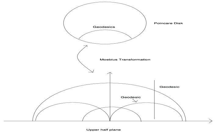
Figure 1: Poincaré disk $\cal D$ and upper half-plane $\mathbb{H}$ with some geodesics. In the upper half-plane, the geodesics correspond to vertical lines and to semi circles centered on the horizon $Im(z)=0$ and in $\cal D$ the geodesics are circles orthogonal to $\cal D$

Solving the Euler-Lagrange equation (3.16), it can be proven that the (hyperbolic) distance (invariant under $PSL(2,{\mathbb{R}})$) between the points $z=x+iy$, $z^{\prime}=x^{\prime}+iy^{\prime}$ on ${\mathbb{H}}^{2}$ is given by (see Appendix A)

$$d(z,z^{\prime})=cosh^{-1}[1+{|z-z^{\prime}|^{2}\over 2yy^{\prime}}]$$ (5.14)

Using this explicit expression for the hyperbolic distance, the VanVleck-Morette determinant is

$$\Delta(z,z^{\prime})={d(z,z^{\prime})\over\sqrt{cosh^{2}(d(z,z^{\prime}))-1}}$$ (5.15)

Using our specific expression for the geodesic distance (5.14), we find that $a_{min}$, the saddle-point, is the following expression

$$a_{min}(f)={\sqrt{{\alpha}^{2}+2\,\alpha\,\nu\,\rho\,q+{\nu}^{2}\,q^{2}}}$$ (5.16)

As $\Delta$ depends only on the geodesic distance $d$ and $d$ is minimised for $a=a_{min}$, we have $ln(\Delta)^{\prime}(a_{min})=0$.

Furthermore, we have (using Mathematica)

$$a_{min}\phi^{\prime\prime}(a_{min})={2d(a_{min})\over\alpha(1-\rho^{2})\sqrt{cosh(d(a_{min}))^{2}-1}}$$ (5.17)

$${\phi^{\prime\prime\prime}(a_{min})\over\phi^{\prime\prime\prime}(a_{min})}=-{3\over a_{min}}$$ (5.18)

$$d(a_{min})=cosh^{-1}({-q\nu\rho-\alpha\rho^{2}+a_{min}(q)\over\alpha(1-\rho^{2})})$$ (5.19)

This above formula (5.19) has already been obtained in [6].

5.3.2 Connection for the $\lambda$-SABR

In the coordinates $[a,f]$, the connection ${\cal A}$ is

$${\cal A}={1\over 2(1-\rho^{2})}({(2\lambda\bar{\lambda}\rho-2\lambda\rho a-\nu a^{2}C^{\prime}(f))\over\nu C(f)a^{2}}df+{(-2\lambda\bar{\lambda}+2\lambda a+\nu\rho a^{2}C^{\prime}(f))\over\nu^{2}a^{2}}da)$$

In the new coordinates $[x,y]$, the above connection is given by

$${\cal A}={\cal A}^{SABR}+{\lambda(\bar{\lambda}\sqrt{1-\rho^{2}}-y)\over\nu^{2}y^{2}\sqrt{1-\rho^{2}}}(\rho dx-\sqrt{1-\rho^{2}}dy)$$ (5.20)

with

$${\cal A}^{SABR} = -{\beta\over 2(1-\rho^{2})(1-\beta)}{dx\over(x+{\rho\over\sqrt{1-\rho^{2}}}y+{\nu f_{0}^{1-\beta}\over(1-\beta)})}\;\;{\mathrm{f}or}\;\;\beta\neq 1$$ (5.21)

$${\cal A}^{SABR} = -{dx\over 2(1-\rho^{2})\nu}\;\;{\mathrm{f}or}\;\;\beta=1$$ (5.22)

The pullback of the connection on a geodesic ${\cal C}$ satisfying $(x-x_{0}(a,f))^{2}+y^{2}=R^{2}(a,f)$ is given by ($\beta\neq 1$ )

$$i^{*}{\cal A}=i^{*}{\cal A}^{SABR}+{\lambda(-\bar{\lambda}\sqrt{1-\rho^{2}}+y)\over\nu^{2}y^{2}}({\rho y\over\sqrt{(R^{2}(a,f)-y^{2})(1-\rho^{2})}}+1)dy$$ (5.23)

and with

$$i^{*}{\cal A}^{SABR}={\beta\over 2(1-\rho^{2})(1-\beta)}{ydy\over\sqrt{R^{2}(a,f)-y^{2}}(\hat{x_{0}}(a,f)+\sqrt{R^{2}(a,f)-y^{2}}+{\rho\over\sqrt{1-\rho^{2}}}y)}$$ (5.24)

with $i:{\cal C}\rightarrow{\mathbb{H}}^{2}$ the embedding of the geodesic ${\cal C}$ on the Poincaré plane and $\hat{x}_{0}=x_{0}+{\nu f_{0}^{1-\beta}\over(1-\beta)}$. We have used that $i^{*}dx=-{ydy\over\sqrt{R^{2}-y^{2}}}$.

Note that the two constants $x_{0}$ and $R$ are determined by using the fact that the two points $z_{1}=-\rho\alpha+i\sqrt{1-\rho^{2}}\alpha$ and $z_{2}=\nu\int_{f_{0}}^{f}{df^{\prime}\over C(f^{\prime})}-\rho a+i\sqrt{1-\rho^{2}}a$ pass through the geodesic curves. The algebraic equations given $R$ and $x_{0}$ can be exactly solved:

$$x_{0}(a,f)={x_{1}^{2}-x^{2}_{2}+y_{1}^{2}-y_{2}^{2}\over 2(x_{1}-x_{2})}$$ (5.25)

$$R(a,f)={1\over 2}\sqrt{{((x_{1}-x_{2})^{2}+y_{1}^{2})^{2}+2((x_{1}-x_{2})^{2}-y_{1}^{2})y_{2}^{2}+y_{2}^{4}\over(x_{1}-x_{2})^{2}}}$$ (5.26)

Using polar coordinates $x-x_{0}=Rcos(\theta)$, $y=Rsin(\theta)$, we obtain that the parallel gauge transport is

$$ln({\cal P})(a)=ln({\cal P}^{SABR})(a)+{\lambda\over\nu^{2}}\int_{\theta_{1}(a)}^{\theta_{2}(a)}(1+Btan(\theta))(sin(x)+A_{0}){cos(x)\over sin(x)^{2}}dx$$ (5.27)

with

$${\cal P}^{SABR}(z,z^{\prime}) = exp(\int_{\theta_{1}}^{\theta_{2}}{\beta\over 2(1-\rho^{2})(1-\beta)}{sin(\theta)d\theta\over(cos(\theta)+{\hat{x}_{0}\over R}+{\rho\over\sqrt{1-\rho^{2}}}sin(\theta))})$$ (5.28)

with $\theta_{i}(a,f)=arctan({y_{i}\over x_{i}-x_{0}})\;,\;i=1,2$, $A(a,f)={\hat{x}_{0}(a,f)\over R(a,f)}$, $B={\rho\over\sqrt{1-\rho^{2}}}$ and $A_{0}=-{\bar{\lambda}\sqrt{1-\rho^{2}}\over R}$. The two integration bounds $\theta_{1}$ and $\theta_{2}$ explicitly depend on $a$ and the coefficient ${\hat{x}_{0}\over R}$. Doing the integration, we obtain (5.3).

Plugging all these results (5.17,5.18,5.19,5.3) in (4.4), we obtain our final expression for the asymptotic smile at the first-order associated to the stochastic $\lambda$-SABR model (5.1).

Remark 5.2 (SABR original formula)

We can now see how the classical Hagan-al asymptotic smile [20] formula can be obtained in the case $\lambda=0$ and show that our formula gives a better approximation.

First we approximate $a_{min}$ by the following expression

$$a_{min}\simeq\alpha+q\rho\nu$$ (5.29)

In the same way, we have

$${\sqrt{cosh(d(a_{min}))^{2}-1}\over d(a_{min})}\simeq 1$$ (5.30)

Furthermore, for $\lambda=0$, the connection (5.3.2) reduces to

$${\cal A}={1\over 2(1-\rho^{2})}(-dln(C(f))+{\rho\over\nu}\partial_{f}Cda)$$ (5.31)

Therefore, the parallel gauge transport is obtained by integrating this one-form along a geodesic $\cal C$

$${\cal P}=exp({1\over 2(1-\rho^{2})}(-ln({C(f)\over C(f_{0})})+\int_{\cal C}{\rho\over\nu}\partial_{f}Cda))$$ (5.32)

The component $f$ of the connection is an exact form and therefore has easily been integrated. The result doesn’t depend on the geodesic but only on the endpoints. However, this is not the case for the component ${\cal A}_{a}$. But by approximating $\partial_{f}^{\prime}C(f^{\prime})\simeq\partial_{f}C(f)$ , the component ${\cal A}_{a}$ becomes an exact form and can therefore be integrated

$$\int_{\cal C}{\rho\over\nu}\partial_{f}Cda\simeq{\rho\over\nu}\partial_{f}C(f)(a-\alpha)$$ (5.33)

Finally, plugging these approximations into our formula (4.4), we reproduce the Hagan-al original formula [20]

$$\sigma_{BS}(f_{0},f,\tau)={ln({f_{0}\over f})\over vol(q)}(1+\sigma_{1}({f+f_{0}\over 2})\tau)$$ (5.34)

with

$$\sigma_{1}(f) = {(\alpha C(f))^{2}\over 24}({1\over f^{2}}+{2\partial_{ff}(C(f))\over C(f)}-({\partial_{f}(C(f))\over C(f)})^{2})+{\alpha\nu\partial_{f}(C(f))\rho\over 4}+{2-3\rho^{2}\over 24}\nu^{2}$$

Therefore, the Hagan-al classical formula corresponds to the approximation of the Abelian connection by an exact form. The latter can be integrated outside the parametrisation of the geodesic curves.

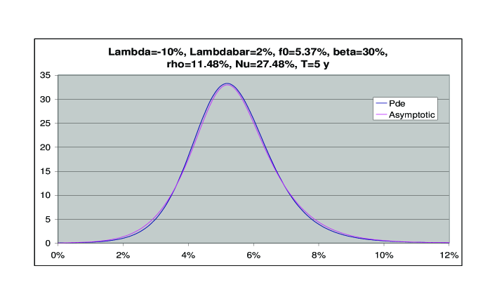
Figure 2: Pdf $p(K,T|f_{0})={\partial^{2}{\cal C}\over\partial^{2}K}$. Asymptotic solution (pink) vs numerical solution (blue) (pde solver). In some cases, the Hagan original formula has been plotted to see the impact of the mean-reversion term.

Remark 5.3 (${\mathbb{H}}^{2}$-model)

In the previous section, we have seen that the $\lambda$-SABR mode corresponds to the geometry of ${\mathbb{H}}^{2}$. This space is particularly nice in the sense that the geodesic distance and the geodesic curves are known. A similar result holds if we assume that $C(f)$ is a general function ($C(f)=f^{\beta}$ for $\lambda$-SABR). In the following, we will try to fix this arbitrary function in order to fit the short-term smile. In this case, we can use our unified asymptotic smile formula at the zero-order. The short-term smile will be automatically calibrated by construction if

$$\sigma_{loc}(f)=C(f)a_{min}(f)$$ (5.35)

$$a_{min}(f)=\alpha^{2}+2\rho\alpha\nu q+\nu^{2}q^{2}$$ (5.36)

$$q=\int_{f_{0}}^{f}{df^{\prime}\over C(f^{\prime})}$$ (5.37)

with $\sigma_{loc}(f)$ the short-term local volatility. By short-term, we mean a maturity date less than $5$ years. Solving (5.35) according to $q$, we obtain

$$\nu q=-\rho\alpha\nu+\sqrt{\alpha^{2}(-1+\rho^{2})+{\sigma_{loc}(f)^{2}\over C(f)^{2}}}$$ (5.38)

and if we derive under $f$, we have ( $\psi(f)={\sigma_{loc}(f)\over C(f)}$)

$${d\psi\over\sqrt{\psi^{2}-\alpha^{2}(1-\rho^{2})}}={\nu\over\sigma_{loc}(f)}df$$ (5.39)

Solving this ODE, we obtain that $C(f)$ is fixed to

$$C(f)={\sigma_{loc}(f)\over\alpha\sqrt{1-\rho^{2}}cosh[\nu\int_{f_{0}}^{f}{df^{\prime}\over\sigma_{loc}(f^{\prime})}]}$$ (5.40)

Using the BBF formula, we have

$$C(f)={f\sigma_{BS}(f)(1-fln({f\over f_{0}}){\sigma_{BS}^{\prime}(f)\over\sigma_{BS}(f)})\over\alpha\sqrt{1-\rho^{2}}cosh[\nu{ln({f\over f_{0}})\over\sigma_{BS}(f)}]}$$ (5.41)

Using this function for the $\lambda$-SABR model, the short term smile is then automatically calibrated.

6 Analytical solution for the SABR model with $\beta=0,1$

6.1 SABR model with $\beta=0$ and ${\mathbb{H}}^{2}$

For the SABR model, the connection ${\cal A}$ and the function $Q$ are given by

$${\cal A}={1\over 2(1-\rho^{2})}(-\partial_{f}ln(C)df+{\rho\over\nu}\partial_{f}Cda)$$ (6.1)

$$Q={a^{2}\over 4}({C\partial_{f}^{2}C}-{(\partial_{f}C)^{2}\over 2(1-\rho^{2})})$$ (6.2)

For $\beta=0$, the function $Q$ and the potential $\cal A$ vanish. Then $p$ satisfies a heat kernel where the differential operator $D$ reduces to the Laplacian on ${\mathbb{H}}^{2}$:

$${\partial p\over\partial\tau^{\prime}} = \Delta_{{\mathbb{H}}^{2}}p$$ (6.3)

$$= y^{2}(\partial_{x}^{2}+\partial_{y}^{2})p$$ (6.4)

Therefore solving the Kolmogorov equation for the SABR model with $\beta=0$ (called SAR0 model) is equivalent to solving this (Laplacian) heat kernel on ${\mathbb{H}}^{2}$. Surprisingly, there is an analytical solution for the heat kernel on ${\mathbb{H}}^{2}$ (6.3) found by McKean [26]. It is connected to the Selberg trace formula [18].

The exact conditional probability density $p$ depends on the hyperbolic distance $d(z,z^{\prime})$ and is given by (with $\tau^{\prime}={\nu^{2}\tau\over 2}$)

$$p(d,\tau^{\prime})=2^{-{5\over 2}}\pi^{-{3\over 2}}\tau^{\prime-{3\over 2}}e^{-{\tau^{\prime}\over 4}}\int_{d(z,z^{\prime})}^{\infty}{be^{-{b^{2}\over 4\tau^{\prime}}}\over(coshb-coshd(z,z^{\prime}))^{1\over 2}}db$$

The conditional probability in the old coordinates $[a,f]$ is

$$p(f,a,\tau^{\prime})dfda={\nu\over(1-\rho^{2})^{1\over 2}}{dfda\over a^{2}C(f)}2^{-{5\over 2}}\pi^{-{3\over 2}}\tau^{\prime-{3\over 2}}e^{-{\tau^{\prime}\over 4}}\int_{d(z,z^{\prime})}^{\infty}{be^{-{b^{2}\over 4\tau^{\prime}}}\over(coshb-coshd(z,z^{\prime}))^{1\over 2}}db$$

We have compared this exact solution (Fig. 3) with a numerical PDE solution of the SAR0 model and found agreement. A similar result was obtained previously in [28, 21] for the conditional probability.

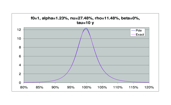
Figure 3: Conditional probability for the SABR model with $\beta=0$ versus numerical PDE.

The value of a European option is (after an integration by parts)

$$C(f,K)=(f-K)^{+}+{1\over 2}\int_{0}^{\tau_{ex}}d\tau\int_{0}^{\infty}daa^{2}p(x_{1}=K,a,\tau|\alpha)$$

In order to integrate over $a$ we use a small trick: we interchange the order of integration over $b$ and $a$. The half space $b\geq d$ with $a$ arbitrary is then mapped to the half-strip $a_{min}\leq a\leq a_{max}$ and $b\geq l_{min}$ where

$$a_{max}-a_{min}=2{\sqrt{\,{(\alpha\,(ch({b})+{\rho}^{2}-ch({b})\,{\rho}^{2})-\nu\,\rho\,q)}^{2}-\,({\alpha}^{2}-2\,\alpha\,\nu\,\rho\,q+{\nu}^{2}\,q^{2})}}$$

$$a_{min}+a_{max}=2\alpha ch(b)+2\alpha\rho^{2}(1-ch(b))+2\nu\rho q$$

$$cosh({l_{min}})={num\over den}$$

with

$$num=-{\alpha}^{2}-2\,{\alpha}^{2}\,{\rho}^{2}-2\,{\alpha}^{2}\,{\rho}^{4}+4\,{\alpha}^{2}\,{\rho}^{6}-6\,\alpha\,\nu\,{\rho}^{3}\,s+4\,\alpha\,\nu\,{\rho}^{5}\,s-3\,{\nu}^{2}\,{\rho}^{2}\,s^{2}$$

$$+2\,{\nu}^{2}\,{\rho}^{4}\,s^{2}+\rho\,\left(-1+2\,{\rho}^{2}\right)\,\left(\alpha\,\rho+\nu\,s\right)\,{\sqrt{{\alpha}^{2}+2\,\alpha\,\nu\,\rho\,\left(-1+2\,{\rho}^{2}\right)\,s+{\nu}^{2}\,\left(-1+2\,{\rho}^{2}\right)\,s^{2}}}$$

$$den=\alpha\,\left(-1+{\rho}^{2}\right)\,\left(1+2\,{\rho}^{2}\right)\,\left(2\,\rho\,\left(\alpha\,\rho+\nu\,s\right)+{\sqrt{{\alpha}^{2}+2\,\alpha\,\nu\,\rho\,\left(-1+2\,{\rho}^{2}\right)\,s+{\nu}^{2}\,\left(-1+2\,{\rho}^{2}\right)\,s^{2}}}\right)$$

Performing the integration according to $a$ leads to an exact solution for the SABR model with $\beta=0$

$$C(f,K)=(f-K)^{+}+{1\over\nu(1-\rho^{2})^{1\over 2}}2^{-{5\over 2}}\pi^{-{3\over 2}}\int_{0}^{{\nu^{2}\tau_{ex}\over 2}}dtt^{-{3\over 2}}e^{-{t\over 4}}\int_{l_{min}}^{\infty}{b(a_{max}-a_{min})e^{-{b^{2}\over 4t}}\over\sqrt{(coshb-coshl_{min})}}db$$

6.2 SABR model with $\beta=1$ and the three-dimensional hyperbolic space ${\mathbb{H}}^{3}$

A similar computation can be carried out for $\beta=1$. Using (6.1), we can show that the potential $\cal A$ is exact, meaning there exists a smooth function $\Lambda$ such that ${\cal A}=d\Lambda$ with $\Lambda={1\over 2(1-\rho^{2})}(-ln(f)+{\rho\over\nu}a)$. Furthermore, using (6.2), we have $Q=-{a^{2}\over 8(1-\rho^{2})}=-{y^{2}\over 8(1-\rho^{2})^{2}}$.

Applying an Abelian gauge transformation $p^{\prime}=e^{\Lambda}p$ (3.11), we find that $p^{\prime}$ satisfies the following equation

$$y^{2}(\partial_{x}^{2}+\partial_{y}^{2}-{1\over 4\nu^{2}(1-\rho^{2})^{2}})p^{\prime}=\partial_{\tau^{\prime}}p^{\prime}$$ (6.5)

How do we solve this equation? It turns out that the solution corresponds in some fancy way to the solution of the (Laplacian) heat kernel on the three dimensional hyperbolic space ${\mathbb{H}}^{3}$. This space can be represented as the upper-half space ${\mathbb{H}}^{3}=\{x=(x_{1},x_{2},x_{3})|x_{3}>0\}$. In these coordinates, the metric takes the following form

$$ds^{2}={(dx_{1}^{2}+dx_{2}^{2}+dx_{3}^{2})\over x_{3}^{2}}$$ (6.6)

and the geodesic distance between two points $x$ and $x^{\prime}$ in ${\mathbb{H}}^{3}$ is given by

$$cosh(d(x,x^{\prime}))=1+{|x-x^{\prime}|^{2}\over 2x_{3}x_{3}^{\prime}}$$ (6.7)

As in ${\mathbb{H}}^{2}$, the geodesics are straight vertical lines or semi-circles orthogonal to the boundary of the upper-half space. An interesting property, useful to solve the heat kernel, is that the group of isometries of ${\mathbb{H}}^{3}$ is $PSL(2,{\mathbb{C}})$ . If we represent a point $p\in{\mathbb{H}}^{3}$ as a quaternion whose fourth components equal zero, then the action of an element $g\in PSL(2,{\mathbb{C}})$ on ${\mathbb{H}}^{3}$ can be described by the formula

$$p^{\prime}=g.p={ap+b\over cp+d}$$ (6.8)

with $p=x_{1}{\bf 1}+x_{2}{\bf i}+x_{3}{\bf j}$.

The Laplacian on ${\mathbb{H}}^{3}$ in the coordinates $[x_{1},x_{2},x_{3}]$ is given by

$$\Delta_{{\mathbb{H}}^{3}}=x_{3}^{2}(\partial_{x_{1}}^{2}+\partial_{x_{2}}^{2}+\partial_{x_{3}}^{2})$$ (6.9)

and the (Laplacian) heat kernel is

$$\partial_{\tau^{\prime}}p^{\prime}=\Delta_{{\mathbb{H}}^{3}}p^{\prime}$$ (6.10)

The exact solution for the conditional probability density $p^{\prime}(d(x,x^{\prime}),t)$, depending on the geodesic distance $d(x,x^{\prime})$, is [17]

$$p^{\prime}(d(x,x^{\prime}),\tau^{\prime})={1\over(4\pi\tau^{\prime})^{3\over 2}}{d(x,x^{\prime})\over sinh(d(x,x^{\prime}))}e^{-\tau^{\prime}-{d(x,x^{\prime})^{2}\over 4\tau^{\prime}}}$$ (6.11)

Let’s apply a Fourier transformation on $p$ along the coordinate $x_{1}$ (or equivalently $x_{2}$)

$$p^{\prime}(x_{1},x_{2},x_{3},x^{\prime},\tau^{\prime})=\int_{-\infty}^{\infty}{dk\over\sqrt{2\pi}}e^{ikx_{1}}\hat{p}(k,x_{2},x_{3},x^{\prime},t)$$ (6.12)

Then $\hat{p}^{\prime}$ satisfies the following PDE

$$\partial_{\tau^{\prime}}\hat{p}^{\prime}=x_{3}^{2}(-k^{2}+\partial_{x_{2}}^{2}+\partial_{x_{3}}^{2})\hat{p}^{\prime}$$ (6.13)

By comparing (6.13) with (6.5), we deduce that the exact solution for the conditional probability for the SABR model with $\beta=1$ is (with $x\equiv x_{2}$, $y\equiv x_{3}$, $k\equiv{1\over 2\nu(1-\rho^{2})}$, $x_{1}^{\prime}=0$)

$$p^{\prime}(x,y,x^{\prime},y^{\prime},\tau^{\prime})=e^{-{1\over 2(1-\rho^{2})}(ln({f\over K})-{\rho\over\nu}(a-\alpha))}\int_{-\infty}^{\infty}{dx_{1}\over\sqrt{2\pi}}{1\over(4\pi\tau^{\prime})^{3\over 2}}{d(x,x^{\prime})\over sh(d(x,x^{\prime}))}e^{-\tau^{\prime}-{d(x,x^{\prime})^{2}\over 4\tau^{\prime}}}e^{-{ix_{1}\over 2\nu(1-\rho^{2})}}$$

A previous solution for the SABR model with $\beta=1$ was obtained by [27], although only in terms of Gauss hypergeometric series.

7 Conclusions and future work

Let’s summarize our findings. By using the heat kernel expansion, we have explained how to obtain a general asymptotic smile formula at the first-order. As an application, we have derived the smile formula for a SABR model with a mean-reversion term. Furthermore, we have shown how to reproduce [19, 20]. In the case of the SABR model with $\beta=0,1$, exact solutions have been found, corresponding to the geometries of ${\mathbb{H}}^{2}$ and ${\mathbb{H}}^{3}$, respectively. We note that these solutions are not easy to obtain without exploiting this connection with hyperbolic geometry.

This geometric framework allows to obtain other analytical solutions for stochastic volatility models. For example, a solution for the heat kernel on a multi-dimensional hyperbolic space ${\mathbb{H}}^{n}$ exists. In a future work, we will show that this space corresponds to a BGM model coupled with a SABR model. Using the general heat kernel expansion on a manifold, we will derive an asymptotic smile for this particular model [24].

8 Appendix: Notions in differential geometry

Riemanian manifold

A real $n$-dimensional manifold is a space which looks like ${\mathbb{R}}^{n}$ around each point. More precisely, $M$ is covered by open sets ${\cal U}_{i}$ (topological space) which are homeomorphic to ${\mathbb{R}}^{n}$ meaning that there is a continuous map $\phi_{i}$ (and its inverse) from ${\mathcal{U}}_{i}$ to ${\mathbb{R}}^{n}$ for each $i$. Furthermore, we impose that the map $\phi_{i,j}=\phi_{i}^{-1}o\phi_{j}$ from ${\mathbb{R}}^{n}$ to ${\mathbb{R}}^{n}$ is $C^{\infty}({\mathbb{R}}^{n})$.

As an example, a two-sphere $S^{2}$ can be covered with two patches: ${\cal U}_{N}$ and ${\cal U}_{S}$, defined respectively as $S^{2}$ minus the north pole, and the south pole. We obtain the map $\phi_{N}$ ($\phi_{S}$) by doing a stereographic projection on ${\mathcal{U}}_{N}$ (${\mathcal{U}}_{S}$). This projection consists in taking the intersection of a line passing through the North (South) pole and a point $p$ on $S^{2}$ with the equatorial plane. We can show that $\phi_{SN}(x,y)=({x\over(x^{2}+y^{2})},-{y\over(x^{2}+y^{2})})$ is $C^{\infty}$ and even holomorphic. So $S^{2}$ is a complex manifold.

Metric

A metric $g_{ij}$ written with the local coordinates $x_{i}$ (corresponding to a particular chart ${\mathcal{U}}_{i}$) allows us to measure the distance between infinitesimally nearby points $x^{i}$ and $x^{i}+dx^{i}$: $ds^{2}=g_{ij}dx^{i}dx^{j}$. If a point $p$ belongs to two charts then the distance can be computed using two different systems of coordinates $x^{i}$ and $x^{i^{\prime}}=f(x^{i})$. However, the result of the measure should be the same, meaning that $g_{ij}dx^{i}dx^{j}=g_{ij}dx^{i^{\prime}}dx^{j^{\prime}}$. We deduce that under a change of coordinates, the metric is not invariant but changes in a contravariant way by $g_{ij}=g_{i^{\prime}j^{\prime}}\partial_{i}x^{i^{\prime}}\partial_{j}x^{j^{\prime}}$.

A manifold endowed with an Euclidean metric is called a Riemannian manifold.

On a $n$-dimensional Riemannian manifold, the measure $\sqrt{g}\prod_{i=1}^{n}dx^{i}$ is invariant under an arbitrary change of coordinates. Indeed the metric changes as $g_{ij}=g_{i^{\prime}j^{\prime}}{\partial x^{i^{\prime}}\over\partial x^{i}}{\partial x^{j^{\prime}}\over\partial x^{j}}$ and therefore $g=det(g_{ij})$ changes as $\sqrt{g}=det({\partial x^{i^{\prime}}\over\partial x^{i}})\sqrt{g^{\prime}}$. Furthermore, the element $\prod_{i=1}^{n}dx^{i}$ changes as $\prod_{i=1}^{n}dx^{i}=det^{-1}({\partial x^{i^{\prime}}\over\partial x^{i}})\prod_{i^{\prime}=1}^{n}dx^{i^{\prime}}$ and we deduce the result.

Line bundle and Abelian connection

Line bundle

A line bundle $\cal L$ is defined by an open covering of $M$, $\{{\cal U}_{\alpha}\}$, and for each $(\alpha,\beta)$, a smooth transition function $g_{\alpha\beta}:{\cal U}_{\alpha}\cap{\cal U}_{\beta}\rightarrow{\mathbb{R}}$ which satisfies the ”cocycle condition”

$$g_{\alpha\beta}g_{\beta\gamma}g_{\gamma\alpha}=1\;\;on\;\;{\cal U}_{\alpha}\cap{\cal U}_{\beta}\cap{\cal U}_{\gamma}$$ (8.1)

A section $\sigma$ of ${\cal L}$ is defined by its local representatives $\sigma$ on each ${\cal U}_{\alpha}$:

$$\sigma|_{{\cal U}_{\alpha}}\equiv\sigma_{\alpha}:{\cal U}_{\alpha}\rightarrow{\mathbb{R}}$$ (8.2)

and they are related to each other by the formula $\sigma_{\alpha}=g_{\alpha\beta}\sigma_{\beta}$ on ${\cal U}_{\alpha}\cap{\cal U}_{\beta}$.

Abelian connection

An Abelian connection $\nabla$ on the line bundle $\cal L$ is a collection of differential operator $\partial_{i}+{\cal A}_{i}^{\alpha}$ on each open set ${\cal U}_{\alpha}$ which transforms according to

$${\cal A}_{i}^{\alpha}={\cal A}_{i}^{\beta}+g_{\alpha\beta}\partial_{i}g_{\alpha\beta}^{-1}\;\;on\;\;{\cal U}_{\alpha}\cap{\cal U}_{\beta}$$ (8.3)

9 Appendix: Laplace integrals in many dimensions

Let $\omega$ be a bounded domain on ${\mathbb{R}}^{n}$, $S:\Omega\rightarrow{\mathbb{R}}$, $f:\Omega\rightarrow{\mathbb{R}}$ and $\lambda>0$ be a large positive parameter. The Laplace’s method consists in studying the asymptotic as $\lambda\rightarrow\infty$ of the multi-dimensional Laplace integrals

$$F(\lambda)=\int_{\Omega}f(x)e^{\lambda S(x)}dx$$ (9.1)

Let $S$ and $f$ be smooth functions and the function $S$ have a maximum only at one interior nondegenerate critial point $x_{0}\in\Omega$. Then in the neighborhood at $x_{0}$ the function $S$ has the following Taylor expansion

$$S(x)=S(x_{0})+{1\over 2}(x-x_{0})^{2}\partial_{x}^{2}S(x_{0})(x-x_{0})+o((x-x_{0})^{3})$$ (9.2)

As $\lambda\rightarrow\infty$, the main contribution of the integral comes from the neighborhood of $x_{0}$. Replacing the function $f$ by its value at $x_{0}$, we obtain a Gaussian integrals where the integration over $x$ can be performed. One gets the leading asymptotic of the integral as $\lambda\rightarrow\infty$

$$F(\lambda)\sim e^{\lambda S(x_{0})}({2\pi\over\lambda})^{n\over 2}[-det(\partial^{2}_{x}S(x_{0}))]^{-1\over 2}f(x_{0})$$ (9.3)

More generally, doing a Taylor expansion at the $n^{\mathrm{t}h}$ order for $S$ (resp. $n-2$-order for $f(x)$) around $x=x_{0}$, we obtain

$$F(\lambda)\sim e^{\lambda S(x_{0})}({2\pi\over\lambda})^{n\over 2}[-det(\partial^{2}_{x}S(x_{0}))]^{-1\over 2}\sum_{k=0}^{\infty}a_{k}\lambda^{-k}$$ (9.4)

with the coefficients $a_{k}$ are expressed in terms of the derivatives of the functions $f$ and $S$ at the point $x_{0}$. For example, at the first-order (in one dimension), we find

$$F(\lambda)\sim\sqrt{{2\pi\over-\lambda S^{\prime\prime}(c)}}e^{\lambda S(x_{0})}\{f(x_{0})+{1\over\lambda}(-{f^{\prime\prime}(x_{0})\over 2S^{\prime\prime}(x_{0})}+{f(x_{0})S^{(4)}(x_{0})\over 8S^{\prime\prime}(x_{0})^{2}}+{f^{\prime}(x_{0})S^{(3)}(x_{0})\over 2S^{\prime\prime}(x_{0})^{2}}-{5S^{\prime\prime\prime}(x_{0})f(x_{0})\over 24S^{\prime\prime}(x_{0})^{3}})\}$$ (9.5)

References

• [1]
• [2] Albanese, C., Campolieti, G., Carr, P., Lipton, A. : Black-Scholes Goes Gypergeometric, Risk magazine, December 2001.
• [3] Avellaneda, M., Boyer-Olson, D., Busca, J., Fritz, P. : Reconstructing the Smile, Risk magazine, October 2002.
• [4] Avramidi, I.V., Schimming, R. :Algorithms for the Calculation of the Heat Kernel Coefficients, hep-th/9510206.
• [5] H. Berestycki, J. Busca, and I. Florent : Asymptotics and calibration of local volatility models, Quantitative finance, 2:31-44, 1998.
• [6] H. Berestycki, J. Busca, and I. Florent : Computing the implied volatility in stochastic volatility models, Comm. Pure Appl. Math., 57, num. 10 (2004), p. 1352-1373.
• [7] Black, F., Scholes, M. :The Pricing of Options and Corporate Liabilities, Journal of Political Economy, 81, 631-659.
• [8] DeWitt, B.S. : Quantum field theory in curved spacetime, Physics Report, Volume 19C, No 6, 1975.
• [9] N.D. Birrell and P.C.W. Davies : Quantum fields in curved space, Cambridge university press, 1982.
• [10] Dupire, B. : Pricing with a Smile, Risk 7, 18-20.
• [11] Eguchi, T., Gilkey, P.B., Hanson, A.J. : Gravitation, Gauge Theories and Differential Geometry, Physcis Report Vol. 66, No 6, december 1980.
• [12] Fouque,J-P, Papanicolaou, G., Sircar, R. : Derivatives in fiancial markets with stochastic volatility, Cambridge University Press, Jul. 2000.
• [13] Gatheral, J. : Case Studies in Financial Modelling lecture notes, 2003.
• [14] Gilkey, P.B. : Invariance Theory, The Heat Equation, and the Atiyah-Singer Index Theorem, http://www.emis.de/monographs/gilkey/.
• [15] P.B. Gilkey, K. Kirsten, J.H. Park, D. Vassilevich : Asymptotics of the heat equation with ’exotic’ boundary conditions or with time dependent coefficients, math-ph/0105009.
• [16] P. Gilkey, K. Kirsten, J.H. Park : Heat Trace asymptotics of a time dependent process, J. Phys. A:Math. Gen Vol 34 (2001) 1153-1168, hep-th/0010136.
• [17] Grigor’yan, A., Noguchi, M. : The Heat Kernel on Hyperbolic Space, Bulletin of LMS, 30 (1998) 643-650
• [18] Gutzwiller, M.C. : Chaos in Classical and Quantum Mechanics, Springer 1990.
• [19] Hagan, P.S., Woodward, D.E. : Equivalent Black Volatilities, Applied mathematical Finance, 6, 147-157 (1999).
• [20] Hagan, P.S., Kumar, D., Lesniewski, A.S., Woodward, D.E. : Managing smile risk, Willmott Magazine pages 84-108, 2002.
• [21] Hagan, P.S., Lesniewski, A.S., Woodward, D.E. : Probability distribution in the SABR model of stochastic volatility, March. 2005, unpublished.
• [22] Heston, S. : A closed-for solution for options with stochastic volatility with applications to bond and currency options, review of financial studies, 6, 327-343.
• [23] Henry-LabordΓ¨re, P. : Stochastic Volatility Model and Hyperbolic Geometry, Working paper Barclays Capital.
• [24] Henry-LabordΓ¨re, P. : Hyperbolic manifold and SABR Libor Model Market, in preparation.
• [25] Hull, J., White, A. : The pricing of options on assets with stochastic volatilities, The Journal of Finance, 42, 281-300.
• [26] MCKean, H.P. : An upper bound to the spectrum of $\Delta$ on a manifold of negative curvature, J. Diff. Geom, 4 (1970) 359-366.
• [27] Lewis, A.L. : Option Valuation under Stochastic Volatility with Mathematica code, Finance Press (2000).
• [28] Lesniewski A. : Working paper, BNPParibas (2001)
• [29] Lesniewski A. : Swaption Smiles via the WKB Method, Seminar Math. fin., Courant Institute of Mathematical Sciences, Feb. 2002.