Mesoscopic oscillations of the conductance of disordered metallic samples as a function of temperature

Abstract

We show theoretically and experimentally that the conductance of small disordered samples exhibits random oscillations as a function of temperature. The amplitude of the oscillations decays as a power law of temperature, and their characteristic period is of the order of the temperature itself.

At low temperatures the conductance of small disordered metallic samples fluctuates from sample to sample. There are two contributions to the amplitude of the fluctuations. The first is associated with a classical effect: the Drude conductivity depends on the concentration of impurities, which fluctuates in space. The second effect is due to electron quantum interference. As a consequence of the latter, the conductance of an individual sample exhibits random oscillations as a function of external magnetic field and chemical potential. The goal of this communication is to point out that the conductance $G(T)$ of an individual mesoscopic metallic sample also oscillates as a function of temperature.

The well known picture of mesoscopic fluctuations of the conductance between samples, and of oscillations of the conductance of individual samples as a function of magnetic field and chemical potential, is as follows. When the sample conductance $G\gg e^{2}/\hbar$ is large and at zero temperature $T=0$, the variance of the interference contribution is universal,

$$\langle(\delta G)^{2}\rangle=\alpha\frac{e^{4}}{\hbar^{2}},$$ (1)

and independent of sample size LeeStone ; Altshuler . Here $\delta G=G-\langle G\rangle$, the brackets $\langle\rangle$ denote averaging over a random scattering potential, and $\alpha$ is a coefficient of order unity which depends on the dimensionality of the sample and its geometry. One can get Eq. 1 by calculating the diagram shown in Fig.1. (We use a standard diagram technique for averaging over random scattering potential abricosov .) The conductance of an individual sample, $G({\bf H})$, exhibits random sample specific oscillations as a function of external magnetic field ${\bf H}$ Web ; LeeStone . We will consider for example the sample geometry shown in the inset of Fig.2, and assume that the sample size $L$ is much larger than the elastic mean free path, $L\gg l$. If the magnetic length $L_{H}\ll L$ and at $T=0$, the amplitude of the oscillations is given by Eq. 1, while their characteristic period is $H^{\ast}\sim\Phi_{0}/L^{2}$, where $\Phi_{0}=h/ec$ is the flux quantum. This statement follows from the magnetic field dependence of the correlation function,

$$\langle(\delta G(\mathbf{H}+\Delta\mathbf{H})\delta G(\mathbf{H}))\rangle\sim\frac{e^{4}}{\hbar^{2}}\Gamma(\Delta\mathbf{H}).$$ (2)

At $\Delta H\gg H^{\ast}$ the correlation function has the asymptotic behavior $\Gamma(\Delta H)\sim L_{\Delta H}/L$ and approaches zero. This can be shown by calculating the diagram in Fig.1, assuming that the inner solid lines correspond to electron Green functions at magnetic field ${\bf H}$ while the outer solid lines correspond to Green functions at ${\bf H}+\Delta{\bf H}$. The oscillations of the conductance as a function of $H$ in the regime where $L_{T}\gg L_{H}\gg L$ were discussed in ZyuzinSpivak . Here $L_{T}=\sqrt{D/T}$, where $D$ is the diffusion coefficient of the metal. For example in the three-dimensional (3d) case the amplitude of the oscillations decays as $L^{-1}_{H}$ while their period is of order $H$. Thus in this regime the typical period of the oscillations decreases while the derivative $dG/dH$ diverges as $H\rightarrow 0$. To get these results one has to assume that the electron diffusion coefficient in the leads is the same as in the sample.

The oscillations mentioned above are of a single-particle interference nature. Contributions to $\delta G$ from electron wave functions with different energies, generally speaking, have different signs. As the temperature $T$ increases, cancellation of contributions at different energies becomes more effective, leading to a decay of the amplitude of the mesoscopic oscillations.

In this article we show that the temperature dependence of the conductance $G(T)$ of an individual sample is actually a non-monotonic function of the temperature $T$ and exhibits random sample specific oscillations. The characteristic period of the oscillations $T^{*}$ is of the order of the temperature itself, that is,

$$T^{*}\sim T.$$ (3)

To prove the existence of the oscillations we calculate the correlation function

$$\langle\delta G(T_{1})\delta G(T_{2})\rangle=\left(\frac{2e^{2}D}{\pi h}\right)^{2}\left(\frac{1}{L}\right)^{4-d}\int_{0}^{\infty}d{\bf q}dt\left[\frac{2}{Dq^{2}+\tau_{\phi}^{-1}}+t\right]\exp[-(Dq^{2}+\tau_{\phi}^{-1})t]B(tT_{1})B(tT_{2}),$$ (4)

where $\tau_{\phi}$ is the electron phase breaking time, and

$$B(z)=\frac{\pi z}{\sinh\pi z}.$$ (5)

It follows from Eq. 4 that in the limit $T\gg T^{\prime}\gg D/L^{2}$

$$\langle{\delta G(T))^{2}}\rangle=\alpha_{1}\frac{e^{4}}{\hbar^{2}}\left\{\begin{array}[]{ll}\frac{D^{1/2}}{T^{1/2}L}&\text{ for $d=3$}\\ \frac{D}{TL^{2}}\ln(\tau_{0}T)&\text{for $d=2$}\end{array}\right.$$ (6)

and

$$\langle\delta G(T^{\prime})\delta G(T)\rangle=\alpha_{1}\frac{e^{4}}{\hbar^{2}}\left\{\begin{array}[]{ll}\frac{D^{1/2}}{T^{1/2}L}(1-0.4(\frac{T^{\prime}}{T})^{2})&\text{ for $d=3$}\\ \frac{D}{TL^{2}}\ln(\tau_{0}T)(1-0.8(\frac{T}{T^{\prime}})^{2})&\text{for $d=2$}\end{array}\right.$$ (7)

Here $\tau_{0}=\min\{\tau_{\phi},D/L^{2}\}$, and $\alpha_{1}$ is a coefficient of order unity which depends on the sample geometry. To get Eq. 6 one can calculate the diagram shown in Fig. 1 where the electron Green functions in the inner and the outer loops are taken at the same temperature $T$. To get Eq. 7 one has to take the Green functions in the inner loop at $T^{\prime}$ and in the outer loop at $T$.

The existence of the oscillations of the conductance $G(T)$ as a function of $T$, and the fact that $\delta G(T)$ changes sign, follow from the facts that the powers of temperature in the denominators of Eq. 6 and Eq. 7 are the same, and that Eq. 7 is independent of $T^{\prime}$ for $T\gg T^{\prime}$. (For example a typical monotonic form $\delta G(T)\sim AT^{-\gamma}$ cannot satisfy both Eq. 6 and Eq. 7 even if the coefficient $A$ has a random sample-specific sign.) A typical realization of the temperature dependence of the conductance has the form

$$\delta G(T)=\langle(\delta G(T))^{2}\rangle^{1/2}F(T),$$ (8)

where the function $F(T)$ randomly oscillates about zero with a characteristic period of order $T$.

In the opposite limit $T\ll D/L^{2}$, (ie. $L_{T}\gg L$), the temperature dependence of $\delta G(T)$ depends on the properties of the leads. In the limit $D_{L}/D\rightarrow\infty$, where $D_{L}$ is the diffusion coefficient in the leads, the function $\delta G(T)$ vanishes monotonically as $T\rightarrow 0$. However, if $D_{L}\sim D$ the $T$-dependence of $G(T)$ has similar features to its $H$-dependence in the limit $L_{T}\gg L_{H}\gg L$ ZyuzinSpivak . That is, $\delta G(T)$ exhibits random oscillations whose amplitude decays as $T\rightarrow 0$. The period of the oscillations for $T\ll D/L^{2}$ is again of order $T^{*}\sim T$. The latter statement follows from the $T$ dependence of the following correlation functions at $T^{\prime}\ll T$,

$$\langle(\frac{d\delta G(T)}{dT})^{2}\rangle\sim\frac{1}{T^{3-d/2}}$$ (9)

and

$$\langle\frac{d\delta G(T^{\prime})}{dT^{\prime}}\frac{d\delta G(T)}{dT}\rangle\sim-\frac{T^{\prime}}{T^{4-d/2}}$$ (10)

which can be obtained by calculation of diagrams in Fig.1 as in ZyuzinSpivak . According to Eqs. 9 and 10 the value of the derivative $dG/dT$ diverges as $T\rightarrow 0$. This is correct as long as $L_{\phi}\gg L_{T}$, where $L_{\phi}=\sqrt{D\tau_{\phi}}$ is the electron phase breaking length. The latter inequality holds if the value of $L_{\phi}$ is determined by electron-electron or electron-phonon scattering Aronov . The qualitative temperature dependence of $\delta G(T)$ in this case is shown in Fig.2.

At very low temperatures the value of $L_{\phi}$ is determined by the paramagnetic impurities in the sample and is temperature independent as long as the Kondo effect and exchange between paramagnetic spins are not significant. In the case $L_{\phi}\ll L_{T}$ the amplitude of the oscillations of $dG/dT$ decays as $T\rightarrow 0$. Thus the typical amplitude of the oscillations of the derivative $dG/dT$ has a maximum when $L_{T}\sim L_{\phi}$; and the total number of oscillations is of order $\ln(T\tau_{s})$, where $\tau_{s}$ is the spin relaxation time.

The oscillations as a function of temperature discussed above should be present in any thermodynamic or transport property of mesoscopic metallic samples.

To test the theory we study some measurements of conductance oscillations in a silicon MOSFET as a joint function of gate voltage $V_{g}$ and temperature $T$. The chosen device has a square channel of length and width $L\sim 1\mu$m. The oxide thickness is 25 nm, giving a gate capacitance per unit area of $8.6\times 10^{11}e$ cm^-2 V^-1. The source and drain contacts are n++ doped silicon. The average conductance, measured by passing an ac current of 5 nA, varies approximately linearly from $19e^{2}/h$ at $V_{g}=4$ V to $26e^{2}/h$ at $V_{g}=5$ V. For practical purposes, the device behaves as a square of disordered 2D electron gas with mobility $\mu\sim 2000$ cm² V^-1 s^-1 and momentum scattering length $l\sim 30$ nm, having 3D metallic contacts. Measurements of conductance oscillations as a function of magnetic field Cobden indicate that the channel is phase coherent at the base temperature of 35 mK achieved on the dilution refrigerator.

The data presented in Fig. 3 are derived from sweeps of $V_{g}$ at a series of temperatures between 35 mK and 1.2 K. (Note that a constant perpendicular magnetic field of 0.1 T was present in all measurements.) A smooth monotonic background variation of the mean conductance $\langle G\rangle$ with $V_{g}$ and $T$ has been subtracted from the raw data, so that the quantity plotted in the figure is the deviation from this background, $\delta G=G-\langle G\rangle$. The sweeps show reproducible oscillations which decay and broaden as $T$ increases, as illustrated in Fig. 3a. The variance $\langle(\delta G)^{2}\rangle$ and correlation gate voltage $V_{g}^{*}$ are plotted against $T$ in Fig. 3b. Fig. 3c is a greyscale plot of $\delta G$ vs $V_{g}$ and $T$, where peaks are light and dips are dark. The appearance of this plot, where individual extrema evolve steadily with $T$, gives us confidence that the data at different temperatures can be compared reliably.

Fig. 3d shows the variation of $\delta G$ with $\log{T}$ at a set of evenly spaced values of $V_{g}$. The curves here are smooth splines passing through the eight temperature points at each $V_{g}$ and extrapolating towards $\delta G=0$ at $T\gg 1.2$ K. For clarity, the actual data points are marked as solid circles on only one of the curves. It is apparent that $\delta G$ oscillates randomly with $T$ on a logarithmic scale, in qualitative accordance with our predictions. Over the factor-of-30 temperature range here, at each gate voltage typically one or two oscillations are resolved. Selected curves have been drawn in bold to illustrate the variety of the oscillatory behavior.

It is quite surprising that these oscillations of the conductance as a function of temperature have never been pointed out in either the theoretical or the experimental literature.

We would like to thank D. Khmelnitskii, L. Levitov, and N. Birge for useful discussions, C. Ford and J. Nichols for help with the experiments, which were performed at the Cavendish Laboratory, and Y. Oowaki of Toshiba for supplying the devices. This work was supported in part by the National Science Foundation under Contracts No. DMR-0228014 (BS).

Figure 1: Diagram describing the correlation function $\langle G({\bf H},T)G({\bf H}^{\prime},T^{\prime})\rangle$. Solid lines correspond to electron Green functions, and thin dashed lines correspond to the correlation function of the random scattering potential.

Figure 2: Typical temperature dependence of the conductance $G(T)$. Insert: schematic diagram of the sample.

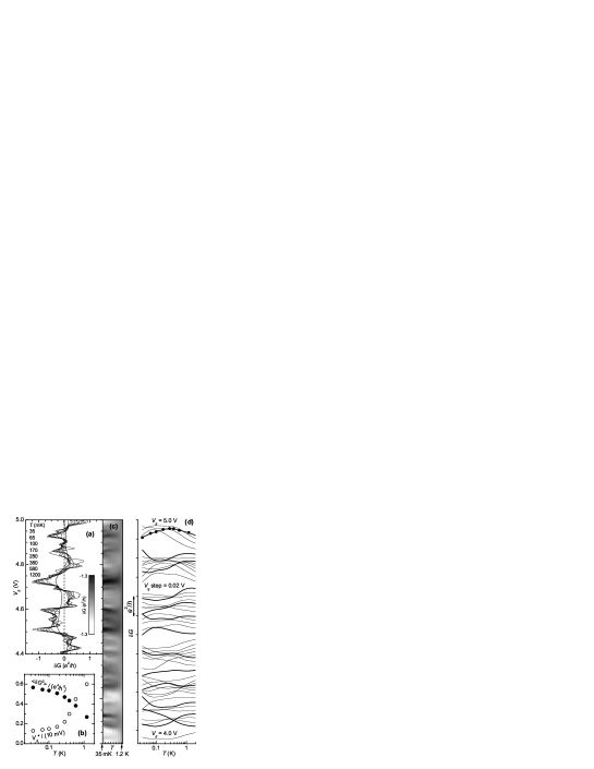
Figure 3: Measurements of the conductance oscillations $\delta G$ in a silicon MOSFET. (a) Gate voltage ($V_{g}$) sweeps at a series of temperatures ($T$) listed at the top left. (b) Variance $\langle(\delta G)^{2}\rangle$ and correlation gate voltage $V_{g}^{*}$ (the half-width of the autocorrelation function) of the oscillations as a function of temperature, obtained by averaging over $V_{g}$. (c) Greyscale plot of $\delta G$ vs $T$ and $V_{g}$. (d) Temperature dependence of $\delta G$ at $V_{g}=4.0,4.02,....5.0$ V, with consecutive sweeps offset vertically by $0.2e^{2}/h$.

References

- (1) P.A. Lee, A.D. Stone, Phys. Rev. Let. 55, 1622, (1985).
- (2) B. Altshuler JETP Lett. 41, 648, (1985).
- (3) C.P. Umbach, S. Washburn, R.B. Laibowitz, R.A. Webb, Phys.Rev. 30, 4048 (1984).
- (4) A.A. Abricosov, L.P. Gorkov, I.E. Dzialoshinski, Methods of quantum field theory in statistical physics., Dover Publ., NY, (1975).
- (5) A. Zyuzin, B. Spivak, JETP 71, 563 (1990).
- (6) B.L. Altshuler, A.G.Aronov, D.Khmelnitsky, J. Phys. C 15, 7367 (1982).
- (7) A. Zyuzin, B. Spivak, JETP Lett. 43, 234 (1986).
- (8) D.H. Cobden, C.H.W. Barnes, and C.J.B. Ford, Phys. Rev. Lett. , 4695 (1999)