Weak Localization in Metallic Granular Media

Abstract

We investigate the interference correction to the conductivity of a medium consisting of metallic grains connected by tunnel junctions. Tunneling conductance between the grains, $e^{2}g_{\rm T}/\pi\hbar$, is assumed to be large, $g_{\rm T}\gg 1$. We demonstrate that the weak localization correction to conductivity exhibits a crossover at temperature $T\sim g^{2}_{\rm T}\delta$, where $\delta$ is the mean level spacing in a single grain. At the crossover, the phase relaxation time determined by the electron-electron interaction becomes of the order of the dwell time of an electron in a grain. Below the crossover temperature, the granular array behaves as a continuous medium, while above the crossover the weak localization effect is largely a single-junction phenomenon. We elucidate the signatures of the granular structure in the temperature and magnetic field dependence of the weak localization correction.

I Introduction

Quantum effects in conduction of two-dimensional disordered electron systems draw attention of both experimentalists and theorists for decades. The interest is motivated in part by the interplay between several fundamental physical phenomena, such as quantum interference, localization, superconductivity, and single-electron tunneling occurring in these systems. The interplay affects the properties of normal conductors Gershenson ; Beenakker ; Sarachik , nominally superconducting films Goldman ; Dynes , and arrays of junctions Fazio . Quantum effects become increasingly important at sheet conductances decreasing towards the fundamental quantum value of $G_{Q}\equiv e^{2}/\pi\hbar$. The interpretation of some of the most intriguing data, however, may depend on whether the investigated conductors are homogeneous or granular. While this question has a definite answer in the case of an array Fazio of lythographically defined junctions, it is less clear for nominally homogeneous deposited metallic films Goldman ; Dynes or electron gases in semiconductor heterostructures Sarachik . Checking the samples homogeneity traditionally involves application of auxiliary techniques, such as local probe spectroscopy Dynes ; Yacoby .

We demonstrate that information about the granularity of a conductor is contained in the temperature and magnetic field dependence of the weak localization (WL) correction to the conductivity. The granular structure of a conductor affects the correction even at high film conductivity, $\sigma_{0}\gg G_{Q}$. While being universal at the lowest temperatures and magnetic fields, the WL correction becomes structure-dependent at higher values of field and temperature. The corresponding crossover temperature is of the order of $(\sigma_{0}/G_{Q})^{2}\delta$, where the mean-level spacing $\delta$ in a single grain is inversely proportional to the grain volume. The field dependence of the WL correction at low temperatures exhibits two crossovers. These are associated with a significant change in structure of closed electron trajectories, allowing for phase-coherent electron motion.

The WL correction in a homogeneous medium originates from the quantum interference of electrons moving along self-intersecting trajectories Gershenson and is proportional to the return probability of an electron diffusing in a disordered medium. In one- or two-dimensional conductors this probability diverges due to the contribution coming from long trajectories. For a fully coherent electron propagation, this divergence would lead to a divergent WL correction. Finite phase relaxation time $\tau_{\phi}$ makes sufficiently long trajectories ineffective for the interference, and limits the correction. In a two-dimensional conductor, the WL correction to conductivity is $\delta\sigma=-(G_{Q}/2\pi)\ln(\tau_{\phi}/\tau)$, where $\tau$ is the electron momentum relaxation time. There are various mechanisms of the electron phase relaxation, some of them being material-specific Birge . The most generic and common for all the conductors mechanism stems from the electron-electron interaction AAK . It yields $1/\tau_{\phi}\sim T(G_{Q}/\sigma_{0})\ln(G_{Q}/\sigma_{0})$ and provides the temperature dependence of the conductivity,

$$\sigma=\sigma_{0}-(G_{Q}/2\pi)\ln(T^{*}/T)$$ (1)

with $T^{*}\sim\sigma_{0}/G_{Q}\tau$. The typical area under an electron trajectory which barely preserves coherence, $L_{\phi}^{2}=D\tau_{\phi}$, depends on the electron diffusion constant. Magnetic field $B$ significantly affects the WL correction if the corresponding magnetic flux through a contour of area $L_{\phi}^{2}$ exceeds the quantum $\Phi_{0}$. This makes the magnetoresistance measurement a useful tool for the investigation of the electron interference.

To model a granular medium, we consider a regular two-dimensional array of grains of size $d$ connected by tunnel junctions. The grains have internal disorder, but are characterized by conductance far exceeding the conductance $g_{\rm T}G_{Q}$ of a single tunnel junction. The classical conductivity of a square array is thus $\sigma_{0}=G_{Q}g_{\rm T}$. It corresponds Beloborodov01 to the effective electron diffusion constant $D=\pi^{-1}g_{\rm T}\delta d^{2}$. In the absence of phase relaxation, an electron may pass through any number of junctions coherently. It will result in a diverging WL correction, just like in a homogeneous conductor. The electron-electron interaction limits the phase relaxation time, yielding $1/\tau_{\phi}\sim T/g_{\rm T}$. As long as the corresponding length $L_{\phi}\sim d\sqrt{g^{2}_{\rm T}\delta/T}$ significantly exceeds $d$, an electron may return to a grain coherently after passing many junctions, and the inhomogeneity of the granular medium is irrelevant. The comparison of $L_{\phi}$ with $d$ defines a crossover temperature,

$$T_{\rm cr}=g^{2}_{\rm T}\delta.$$ (2)

Roughly, above the crossover temperature the electron trajectories contributing to the WL do not cross more than a single junction. In this regime granular medium behaves similarly to a single grain connected to highly conducting leads by tunnel junctions of conductance $g_{\rm T}$.

The WL correction at $T\gtrsim T_{\rm cr}$ comes from electron trajectories that pass through a single tunnel junction. Electrons moving along longer trajectories, which include more junctions, have much smaller probability of a phase-coherent return. We find that already the shortest inter-grain trajectories (see Fig. 2 in Section IV) provide the temperature dependence of the WL correction,

$$\delta\sigma_{\rm WL}=-A\frac{T_{\rm cr}}{T},$$ (3)

with $A$ being a geometry-dependent coefficient of order one. In deriving Eq. (3), we assume that $g_{\rm T}$ is much smaller than the number of channels in the inter-grain tunnel junction, although $g_{\rm T}\gg 1$.

Equation (3) does not account for the phase relaxation rate within the grains. At a sufficiently high temperature $T\gtrsim T^{*}$ the latter exceeds the electron escape rate $g_{\rm T}\delta$ from a grain, which leads to a suppression of the WL correction below the value Eq. (3). The characteristic scale $T^{*}$ here depends on the intra-grain phase relaxation mechanism. Assuming that it is due to the electron-electron interaction Sivan , and that the dimensionless conductance of the grain $g_{\rm gr}$ is large, $g_{\rm gr}\gtrsim g_{\rm T}^{2}$, we find

$$T^{*}\sim T_{\rm cr}\frac{g_{\rm gr}}{g_{\rm T}^{2}}\sqrt{g_{\rm T}}.$$ (4)

In a more exotic case of a smaller grain conductance, $g_{\rm T}^{2}\gg g_{\rm gr}\gg g_{\rm T}$, the temperature $T^{*}$ still exceeds significantly $T_{\rm cr}$, but the specific relation between the two temperature scales depends on the grain shape, and is different for disk-like or dome-like grains.

We turn now to the discussion of the magnetic field effect on the weak localization in the granular medium. To determine the characteristic field suppressing the interference correction to conductivity, we need to estimate the directed area covered by a typical closed electron trajectory ABG . For a single grain, such area is of the order $d^{2}\sqrt{g_{\rm gr}/g_{T}}$ and is limited by the electron dwelling time. At low temperatures, $T\ll T_{\rm cr}$, the number of grains visited by an electron having a typical closed trajectory, is of the order of $T_{\rm cr}/T$. The single-grain directed areas have random signs, so the estimate for the full directed area is

$$S_{\rm eff}\sim d^{2}\sqrt{\frac{T_{\rm cr}g_{\rm gr}}{Tg_{\rm T}}}+d^{2}\frac{T_{\rm cr}}{T}\,.$$ (5)

The first term here corresponds to the sum of the directed areas under the electron trajectory within the grains visited by electron; the second, conventional Gershenson , term comes from the fact that the “visited” grains form a closed contour of an area $L_{\phi}^{2}$, see Fig. 1. The characteristic level of the field necessary to affect $\delta\sigma_{\rm WL}$ is found from the condition $S_{\rm eff}B_{\phi}\sim\Phi_{0}$. We see now, that even within the temperature range $T\lesssim T_{\rm cr}$, the granularity of the material matters.

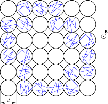
Figure 1: A typical diffusive trajectory in a granular array. The directed area $S_{\rm eff}$ consists of two components. The first one is the combined contribution of separate grains, see the first term in Eq. (5). The second component is the area under the coarse-grained trajectory, which is the counterpart of the directed area under an electron trajectory in a homogeneous disordered sample.

At the lowest temperatures the characteristic field coincides with that of a film with the corresponding value of diffusion coefficient,

$$B_{\phi}\sim\frac{\Phi_{0}}{d^{2}}\frac{T}{T_{\rm cr}},\quad T\ll T_{\rm cr}\frac{g_{T}}{g_{\rm gr}}.$$ (6)

At higher temperatures, the characteristic field is

$$B_{\phi}\sim\frac{\Phi_{0}}{d^{2}}\sqrt{\frac{Tg_{\rm T}}{T_{\rm cr}g_{\rm gr}}}\;,\quad T_{\rm cr}\frac{g_{T}}{g_{\rm gr}}\ll T\ll T_{\rm cr}.$$ (7)

The higher the applied field, the shorter are the trajectories contributing to the interference correction, and the smaller the correction is. Such trajectories span only a single grain provided the field $B$ is of the order or higher than

$$B_{\phi}^{\rm sg}=\frac{\Phi_{0}}{d^{2}}\sqrt{\frac{g_{\rm T}}{g_{\rm gr}}}.$$ (8)

At $B\gg B_{\phi}^{\rm sg}$, even the single-grain Cooperon is suppressed. Consequently, Eq. (8) defines the characteristic field suppressing at $T\gtrsim T_{\rm cr}$ the WL correction Eq. (3), which stems from the transitions within the closest grain pairs.

To develop a quantitative theory of the interference correction, we derive the expression for the weak localization correction and adapt the Cooperon equation for granular medium.

II Conductance and weak localization in a granular array

Tunnel junctions between metallic grains are described adequately by a model with an infinitely large number of weakly-conducting channels. Within this model, one can use the tunneling Hamiltonian formalism for evaluation of the conductivity of the granular array. In this formalism, tunneling between the grains $m$ and $n$ is described by the Hamiltonian

$$\hat{H}_{\rm T}=\sum_{\alpha\beta\sigma}t_{\alpha\beta}e^{iV_{mn}t}\hat{a}_{\alpha\sigma}^{\dagger}\hat{a}_{\beta\sigma}+h.c.=\sum_{\sigma}\int_{m}d\bm{r}_{1}$$ (9)

$$\times\int_{n}d\bm{r}_{2}t(\bm{r}_{1},\bm{r}_{2})e^{iV_{mn}t}\hat{\psi}_{m\sigma}^{\dagger}(\bm{r}_{1})\hat{\psi}_{n\sigma}(\bm{r}_{2})+h.c.\ ,$$

where the points $\bm{r}_{1}$ and $\bm{r}_{2}$ belong to the grains $m$ and $n$, respectively, $V_{mn}$ is the voltage applied to the barrier, $\alpha\in m$ and $\beta\in n$ are exact single-particle states, and $\sigma$ is the spin index. In the limit of thin barrier, the tunnel amplitude $t$ significantly deviates from zero only if the vectors $\bm{r}_{1}$ and $\bm{r}_{2}$ refer to two closest to each other points at opposite sides of the interface,

$$t(\bm{r}_{1},\bm{r}_{2})=a\delta(y-y^{\prime})\partial_{z}\partial_{z^{\prime}}\delta(z)\delta(z^{\prime}).$$ (10)

Here the coordinate $y$ runs along the interface $S$, and transverse coordinates $z$ in the grain $m$ and $z^{\prime}$ in the grain $n$ are defined in such a way that at the interface $z=z^{\prime}=0$. (We wrote Eq. (10) for the planar geometry, generalization to three-dimensional arrays is straightforward). The constant $a$ is of the order of magnitude of $\sqrt{{\cal T}}/\nu k_{F}$, where $\nu$ is the electron density of states of the material of the grains, and ${\cal T}$ is the transmission coefficient of the barrier. The numerical factor in $a$ can be related to the measurable quantity, the barrier conductance $g_{\rm T}$. Using Eq. (10), one may express the tunnel amplitude in terms of the eigenfunctions $\chi_{\alpha}$ and $\chi_{\beta}$ of an electron in the grains $m$ and $n$, respectively (see, e.g., Ref. Houzet, ),

$$t_{\alpha\beta}=a\int_{S}dy\partial_{z}\chi^{*}_{\alpha}(y,z)\partial_{z^{\prime}}\chi_{\beta}(y,z^{\prime})|_{z=z^{\prime}=0}\ .$$ (11)

The current through the contact is defined as $\hat{I}=-e\hat{\dot{N}}_{m}=-ie[\hat{H}_{\rm T},\hat{N}_{m}]$, where $\hat{N}_{m}$ is the number of particles in the grain $m$,

$$\hat{N}_{m}=\sum_{\alpha\sigma}\hat{a}^{\dagger}_{\alpha\sigma}\hat{a}_{\alpha\sigma}\ .$$

Calculating the average current through the barrier, we obtain

$$I(t)=-e\ \mbox{Re}\int d\bm{r}_{1}d\bm{r}_{2}\left\{t(\bm{r}_{1},\bm{r}_{2})G^{K}_{nm}(\bm{r}_{2},\bm{r}_{1},t,t)e^{iV_{mn}t}\right.$$

$$\left.-t^{*}(\bm{r}_{1},\bm{r}_{2})G^{K}_{mn}(\bm{r}_{2},\bm{r}_{1},t,t)e^{-iV_{mn}t}\right\}\ ,$$

where $G^{K}$ is the Keldysh component of the matrix Green’s function, and the subscripts $m$ and $n$ are introduced for convenience, in order to indicate which grain points $\bm{r}_{1}$ and $\bm{r}_{2}$ belong to. We need now to calculate the function $G^{K}$ by perturbation theory in tunneling Hamiltonian. Let us first discuss the first order and calculate the average conductance. Using the standard technique Rammer , we obtain for the current in the frequency representation (terms which do not depend on the time difference would correspond to the Josephson effect and thus are dropped)

$$I(\omega) = 2e\ \mbox{Re}\int d\bm{r}_{1}\dots d\bm{r}_{4}\frac{d\omega}{2\pi}t^{*}(\bm{r}_{1},\bm{r}_{2})t(\bm{r}_{3},\bm{r}_{4})$$

$$\times \mbox{Tr}\left[\hat{\tau}_{x}\hat{G}_{m}(\bm{r}_{1},\bm{r}_{3},\omega+eV_{mn})\hat{G}_{n}(\bm{r}_{4},\bm{r}_{2},\omega)\right],$$

where $\tau_{x}$ is the Pauli matrix in the Keldysh space, $G_{n}\equiv G_{nn}$, and we use the standard representation

$$\hat{G}=\left(\begin{array}[]{cc}G^{R}&G^{K}\\ 0&G^{A}\end{array}\right)\ .$$

In the linear regime, it suffices to use the equilibrium function here, $G^{K}(E)=\tanh(E/2T)(G^{R}(E)-G^{A}(E))$. Expressing the Green’s functions in terms of the exact eigenfunctions, calculating the energy integrals, and substituting the transmission amplitudes (10), we obtain $I=\sigma V_{mn}$ for the inter-grain current, and $\sigma=(e^{2}/\pi)g_{\rm T}$ for the Drude conductivity of the granular array. The introduced here dimensionless inter-grain tunneling conductance is

$$g_{\rm T}=4\pi^{2}|a|^{2}\int_{S}dydy^{\prime}$$

$$\left|\left\langle\sum_{\alpha}\partial_{z}\chi_{\alpha}(yz)\partial_{z^{\prime}}\chi^{*}_{\alpha}(y^{\prime}z^{\prime})|_{z=z^{\prime}=0}\delta(\xi_{\alpha})\right\rangle\right|^{2}$$

$$=4|a|^{2}\int_{S}dydy^{\prime}\left[\partial_{z}\partial_{z^{\prime}}\mbox{\rm Im}\ \left\langle G^{R}(yz;y^{\prime}z^{\prime})\right\rangle|_{z=z^{\prime}=0}\right]^{2}\ ,$$

where $\xi_{\alpha}$ are the exact energy eigenvalues measured from the Fermi level in a grain, and angular brackets mean impurity averaging within a grain (the eigenfunctions in different grains are not correlated). In the last equation, $\langle G^{R}\rangle$ is the impurity-averaged Green’s function evaluated at the Fermi energy. It is represented as the density of states $\nu$ multiplied with a dimensionless function rapidly decaying with the distance $y-y^{\prime}$. The characteristic length of that decay is given by the Fermi wavelength, and the integral in Eq. (II) is converging rapidly. Therefore the dimensionless function of $y-y^{\prime}$ may be evaluated within the free-electron approximation Houzet . The precise shape of this function is not important for our purposes. Equation (II) thus relates the tunnel conductance to the previously introduced constant $a$.

Figure 2: Second-order correction to the conductivity. Black circles represent the tunnel amplitudes, and dashed lines denote impurity scattering inside the grains

We proceed now with the evaluation of weak localization correction. The next-order contribution to the current (Fig. 2) contains four tunnel amplitudes and four Green’s functions with the Keldysh structure $\mbox{Tr}\ (\hat{\tau}_{x}\hat{G}\hat{G}\hat{G}\hat{G})$, where $\hat{G}$ is the matrix Green’s function in the Keldysh space. The trace of a product of several Green’s function can only have the following structure: several first functions are retarded, followed by one Keldysh function and then a number of advanced functions. Thus, we have the combination of the type $G^{K}G^{A}G^{A}G^{A}+G^{R}G^{K}G^{A}G^{A}+G^{R}G^{R}G^{K}G^{A}+G^{R}G^{R}G^{R}G^{K}$. However, the second and third terms in this combination are considerably greater than the other two, since the impurity scattering inside the grains is the most effective if the impurity line connect advance and retarded, advanced and Keldysh, and Keldysh and retarded Green’s functions, but not two retarded or two advanced ones. Thus, retaining only these two termsAAK ; AA , we express the weak localization correction in terms of the Cooperon $C_{mn}$ in the time representation,

$$\delta\sigma_{\rm WL}=-\frac{2e^{2}}{\pi}\mbox{Re}\ \int d\bm{r}_{1}\dots d\bm{r}_{4}t^{*}(\bm{r}_{1},\bm{r}_{2})t(\bm{r}_{3},\bm{r}_{4})$$

$$\times\int_{-\infty}^{\infty}dtC_{mn}(\bm{r}_{1},\bm{r}_{4};\bm{r}_{3},\bm{r}_{2};t,-t)\ ,$$ (15)

where the subscripts of the Cooperon indicate that it starts and ends in the grains $m$ and $n$, respectively. Note that due to the structure of the tunneling amplitudes $t(\bm{r},\bm{r}^{\prime})$, point $\bm{r}_{1}$ is just across the barrier from point $\bm{r}_{2}$ and similarly point $\bm{r}_{3}$ is across the barrier from point $\bm{r}_{4}$. The Cooperon $C$ can be presented in the form

$$C_{mn}(\bm{r}_{1},\bm{r}_{4};\bm{r}_{2},\bm{r}_{3})=\frac{\pi}{\nu}\mbox{Im}\ \left\langle G^{R}_{m}(\bm{r}_{1}-\bm{r}_{4})\right\rangle$$

$$\times\mbox{Im}\left\langle G^{R}_{n}(\bm{r}_{2}-\bm{r}_{3})\right\rangle\tilde{C}_{mn}(\bm{r}_{1},\bm{r}_{3})\ .$$

Rapid decay of functions $\langle G^{R}\rangle$ with the distance between the corresponding arguments makes points in pairs $\bm{r}_{1}$, $\bm{r}_{4}$ and $\bm{r}_{2}$, $\bm{r}_{3}$ in the spatial integral of Eq. (II) to be within the Fermi wavelength from each other. On the other hand, the Cooperon $\tilde{C}(\bm{r}_{1},\bm{r}_{3})$ is generally a long-range function. Provided we are interested in times long compared to the intra-grain diffusion time, $\tilde{C}$ almost does not change while its coordinates vary within respective grains. However, $\tilde{C}_{mn}(\bm{r}_{1},\bm{r}_{3})$ with $m\neq n$ may differ significanlty from the value of single-grain Cooperon ($m=n$). Substituting this coarse-grained Cooperon $\tilde{C}_{mn}$ into Eq. (II) and taking into account Eqs. (10) and (II), we obtain

$$\delta\sigma_{\rm WL}=\frac{e^{2}g_{\rm T}}{2\pi\nu^{2}}\mbox{Re}\int_{-\infty}^{\infty}dt\tilde{C}_{mn}(t,-t)\$$ (16)

with $m$ and $n$ being the neighboring grains. Note that Eq. (16) is valid for any dimension, not just in 2D.

The form (16) of weak localization correction is valid provided the phase coherence between the grains barely survives, and $\tilde{C}_{mn}\ll\tilde{C}_{nn}$ at $m\neq n$. This limit is realized at a sufficiently high temperature, $T\gg T_{\rm cr}$. Note also that the performed derivation, unlike the consideration of, e.g., Ref. VA, assumes the limit of large number of channels taken at fixed value of $g_{\rm T}$.

To consider phase relaxation in a granular array, we derive now the proper equation for $\tilde{C}_{nm}$ in a granular medium.

III Cooperon in a granular array

Cooperon describes the probability amplitude of electron return and in the case of a homogeneous medium with electron diffusion coefficient $D$ obeys the equation

$$\left\{\frac{\partial}{\partial t}-D\left[\frac{\partial}{\partial\bm{r}}-i\frac{e}{c}\bm{A}(\bm{r},-t/2)-i\frac{e}{c}\bm{A}(\bm{r},t/2)\right]^{2}\right\}\tilde{C}(\bm{r},\bm{r}^{\prime};t,t^{\prime})=\delta\left(\bm{r}-\bm{r}^{\prime}\right)\delta(t-t^{\prime}).$$ (17)

Here the vector potential $\bm{A}$ accounts for the fluctuating electric fields representing the effect of electron-electron interactions, and should be considered as a Gaussian classical random variable with zero average.

In order to adapt Eq. (17) to the case of a granular medium, it is convenient to perform a gauge transformation, after which the fluctuating fields are described by a random scalar potential $\varphi(\bm{r},t)$, rather than by the vector potential $\bm{A}(\bm{r},t)$,

$$\bm{A}(\bm{r},t)=c\int^{t}\nabla_{\bm{r}}\varphi(\bm{r},t^{\prime})dt^{\prime}$$

(we assume there are no magnetic fields applied to the system). Defining the Cooperon $C(\bm{r},\bm{r}^{\prime};t,t^{\prime}))$ in the new gauge by the relation

$$\tilde{C}(\bm{r},\bm{r}^{\prime};t,t^{\prime})=C(\bm{r},\bm{r}^{\prime};t,t^{\prime}))$$ (18)

$$\times\exp\left\{ie\int^{t/2}\varphi(\bm{r},t^{\prime\prime})dt^{\prime\prime}-ie\int^{t^{\prime}/2}\varphi(\bm{r}^{\prime},t^{\prime\prime})dt^{\prime\prime}\right.$$

$$\left.+ie\int^{-t/2}\varphi(\bm{r},t^{\prime\prime})dt^{\prime\prime}-ie\int^{-t^{\prime}/2}\varphi(\bm{r}^{\prime},t^{\prime\prime})dt^{\prime\prime}\right\}\ \ ,$$

we obtain the equation

$$\left\{\frac{\partial}{\partial t}+\frac{ie}{2}\varphi(\bm{r},t/2)-\frac{ie}{2}\varphi(\bm{r},-t/2)-D\frac{\partial^{2}}{\partial\bm{r}^{2}}\right\}C(\bm{r},\bm{r}^{\prime};t,t^{\prime})=\delta\left(\bm{r}-\bm{r}^{\prime}\right)\delta(t-t^{\prime}).$$ (19)

Note that $\tilde{C}(\bm{r},\bm{r};t,-t)=C(\bm{r},\bm{r};t,-t)$, and thus $C$ can be used instead of $\tilde{C}$ in for evaluation of the WL correction (16).

Returning to the consideration of a granular array, we assume that the intra-grain conductance is high, $g_{\rm gr}\gg g_{\rm T}$. Then the fluctuating potential $\varphi(\bm{r},t)$ does not vary from point to point within a single grain, while exhibiting random fluctuations of the inter-grain potential differences. This allows us to coarse-grain function $\varphi(\bm{r},t)$, replacing its dependence on ${\bm{r}}$ by the dependence on the grain number $n$. We also can simplify the spatial dependence of the Cooperon $C(\bm{r},\bm{r}^{\prime};t,t^{\prime}))$, in case we are interested in times long compared to the intra-grain diffusion time. Indeed, in that case $C$ does not change while $\bm{r}$ or $\bm{r}^{\prime}$ vary within a grain. Therefore, the dependence of the Cooperon on the coordinates may be replaced by the dependence on the grain numbers $n$ and $n^{\prime}$ which the coordinates $\bm{r}$ and $\bm{r}^{\prime}$ belong to. The resulting coarse-grained equation for the Cooperon reads:

$$\left\{\frac{\partial}{\partial t}+\frac{ie}{2}\varphi_{n}(t/2)-\frac{ie}{2}\varphi_{n}(-t/2)+N\frac{g_{\rm T}\delta}{\pi}\right\}C_{nn^{\prime}}(t,t^{\prime})$$

$$-\frac{g_{\rm T}\delta}{\pi}\sum_{k}C_{kn^{\prime}}(t,t^{\prime})=\delta_{nn^{\prime}}\delta(t-t^{\prime}).$$ (20)

Here $N$ is the number of junctions to a single grain (i.e., the coordination number of the lattice of grains; $N=4$ for a two-dimensional square lattice), and the summation in the last term on the left-hand side runs over $N$ nearest neighbors $k$ of the grain $n$.

Equations (16) and (III) provide a convenient starting point for evaluation of the weak localization correction at temperatures $T\ll T^{*}$, see Eq. (4). At higher temperatures, the spatial dispersion of the fluctuating potentials and of the Cooperon inside a grain becomes important.

The temperature domain $T\lesssim T^{*}$ is separated in two characteristic regions by the scale $T_{\rm cr}$, Eq. (2). At $T\ll T_{\rm cr}$, the dependence of Cooperon $C$ on $n-n^{\prime}$ is smooth, and the finite difference equation (III) can be replaced by the corresponding differential equation, which essentially returns one to the continuous-medium case, see Eq. (19). Weak localization corrections in this case are studied in detail in Refs. AAK, ; AA, . Below we concentrate on the temperatures above the crossover.

IV Quantum correction to conductivity above the crossover temperature

In the temperature regime of interest,

$$T^{*}\gg T\gtrsim T_{\rm cr},$$ (21)

as we have explained in the Introduction, electron trajectories are classified according to the number of tunnel junctions they cross — the longer are the trajectories, the less significant are their contributions. It means that the matrix $C_{nn^{\prime}}$ rapidly decays away from the diagonal. The biggest matrix elements are $C_{nn}$, and the most important trajectories are those which do not leave the grain. Eq. (16) implies that these trajectories do not contribute to the weak localization correction, and one needs to consider the next-order contribution coming from trajectories crossing a single junction once. This leads us to Eq. (3) and also allows us to verify the existence of the crossover temperature Eq. (2).

At $T\gg T_{\rm cr}$ we expect strong fluctuations of the potential differences between the grains, making coherent returns of an electron to the grain of its origin improbable. The returns are described by the term in Eq. (III) containing the sum over $k$. Neglecting that term, we find for the diagonal component $C_{nn}(tt^{\prime})$ of the Cooperon

$$C_{nn}^{(0)}(t,t^{\prime})=\theta(t-t^{\prime})\exp\left\{-N\frac{g_{\rm T}\delta}{\pi}(t-t^{\prime})\right.$$

$$-\left.ie\int_{t^{\prime}/2}^{t/2}\varphi_{n}(t^{\prime\prime})dt^{\prime\prime}-ie\int_{-t^{\prime}/2}^{-t/2}\varphi_{n}(t^{\prime\prime})dt^{\prime\prime}\right\}.$$ (22)

The phase factors here reflect the specific gauge we used in Eq. (III).

Next, we write the Cooperon equation (III) for the nearest-neighbor sites $m$ and $n$,

$$\left\{\frac{\partial}{\partial t}+\frac{ie}{2}\varphi_{m}(t/2)-\frac{ie}{2}\varphi_{m}(-t/2)+N\frac{g_{\rm T}\delta}{\pi}\right\}C_{mn}(t,t^{\prime})$$

$$=\frac{g_{\rm T}\delta}{\pi}C^{(0)}_{nn}(t,t^{\prime}).$$ (23)

The terms with $C_{n^{\prime},n}$ describing the grains $n^{\prime}$ separated from $n$ by two tunnel junctions, are small and can be omitted in this approximation. Using Eqs. (IV) and (IV), we obtain for the neighboring grains $m$ and $n$

$$C_{mn}(t,t^{\prime})=\frac{g_{\rm T}\delta}{\pi}\theta(t-t^{\prime})\exp\left\{-N\frac{g_{\rm T}\delta}{\pi}(t-t^{\prime})\right\}\int_{t^{\prime}}^{t}dt_{1}$$

$$\times\exp\left\{-ie\int_{t^{\prime}/2}^{t_{1}/2}\varphi_{n}(t^{\prime\prime})dt^{\prime\prime}-ie\int_{-t^{\prime}/2}^{-t_{1}/2}\varphi_{n}(t^{\prime\prime})dt^{\prime\prime}\right.$$

$$\left.+ie\int_{t/2}^{t_{1}/2}\varphi_{m}(t^{\prime\prime})dt^{\prime\prime}+ie\int_{-t/2}^{-t_{1}/2}\varphi_{m}(t^{\prime\prime})dt^{\prime\prime}\right\}\ .$$ (24)

This expression has to be averaged over the Gaussian fluctuations of the field $\varphi$. Its correlation function is defined by the fluctuation-dissipation theorem and reads AB02

$$e^{2}\langle\varphi\varphi\rangle(\bm{q},\omega)=-\mbox{\rm Im}\ \frac{2T}{\omega}\frac{1}{\Pi(\bm{q},\omega)},$$

where $\Pi$ is the polarization operator, calculated for a granular medium in Ref. Beloborodov01, . In the space-time representation, we obtain

$$e^{2}\left\langle\varphi_{n}(t)\varphi_{n^{\prime}}(t^{\prime})\right\rangle=\frac{\pi Td^{2}}{g_{\rm T}}\delta(t-t^{\prime})$$ (25)

$$\times \int\frac{d\bm{q}}{(2\pi)^{d}}\frac{e^{i\bm{q}(\bm{n}-\bm{n^{\prime}})}}{\sum_{a}(1-\cos q_{a}d)},$$

where the summation in the denominator is carried over all available Cartesian components $a=x,y$, and ${\bm{q}}_{a}$ are the basis vectors of square lattice of grains.

Performing the averaging in Eq. (IV) with the help of Eq. (25) is cumbersome but straightforward, since for Gaussian fields $\langle\exp(i\dots)\rangle=\exp(-\langle\dots\rangle/2)$. For the weak localization correction, we obtain

$$\frac{\delta\sigma_{\rm WL}}{\sigma_{0}}=-A\frac{g_{\rm T}\delta}{T},$$ (26)

$$A\equiv\frac{1}{N^{2}V}\sum_{a}\left(\int\frac{d\bm{q}}{(2\pi)^{d}}\frac{1-\cos q_{a}d}{\sum_{a}(1-\cos q_{a}d)}\right)^{-1}\,,$$

where $V$ is the volume of the grain ($V=d^{2}$ in 2D). Note that the interference correction Eq. (26) depends on temperature and on the type of lattice the grains form. The dependence on the lattice type comes through the coefficient $A$; for a square 2D lattice we find $A=1/4$. One can easily generalize the evaluation of $A$ onto the case of a triangular and more complicated lattices, eventually even describing disordered media like ceramics.

V Magnetic field effect

As the estimate Eq. (5) suggests, the action of the magnetic field on Cooperon is two-fold. A part of the Cooperon suppression comes from the intra-grain electron motion, and another part stems from the magnetic field effect on the inter-grain coherence. Since $g_{\rm gr}\gg g_{\rm T}$, the interesting range of the fields corresponds to a small flux penetrating a grain, $Bd^{2}\ll\Phi_{0}$. We can then consider the effect of magnetic field on the Cooperon within a grain perturbatively. To implement the perturbation theory, it is convenient to use a “tailored” to the grains shape gauge of the magnetic field $B$. For definiteness, we concentrate on the case of a two-dimensional array of “flat” grains connected by point-like tunneling contacts, see Fig. 1. We define the gauge for the points within the grains by the relations

$${\bm{A}}_{\phi}({\bf r})={\bm{\tau}}\times\nabla\psi_{n}({\bf r})+{\bm{A}}_{n}\,,\;\nabla^{2}\psi_{n}=B\,,\;\psi_{n}({\bm{r}}\in b_{n})=0.$$ (27)

Here ${\bm{\tau}}$ is the normal to the plane of the grains, and $b_{n}$ is the boundary of the $n$–th grain. The second and third relations in Eq. (27) fully define the boundary problem for a scalar function $\psi_{n}({\bm{r}})$. The constants ${\bm{A}}_{n}$ are tuned in such way that the vector-potential is continuous at the points of contact between the grains. Up to a discrete analogue of the gradient of a scalar function, these constants are determined fully by the solution of the boundary problems for all $\psi_{m}({\bm{r}})$. It is clear that the discrete version of curl applied to ${\bm{A}}_{n}$ must be equal ${\bm{B}}$ upon averaging over the array; the characteristic difference $A_{n}-A_{m}$ for two nearby junctions is of the order $A_{n}-A_{m}\sim B\cdot d$.

In the definition of the Cooperon, it is convenient to present again the coordinates as pairs $\{{\bm{r}},n\}$ and $\{{\bm{r}}^{\prime},n^{\prime}\}$ which point explicitly to the label of grains the two points ${\bm{r}},{\bm{r}}^{\prime}$ belong to. In addition, we multiply the Cooperon defined in Eq. (18) by yet one more gauge factor,

$$C_{mn}(\bm{r},\bm{r}^{\prime};t,t^{\prime})=C^{\phi}_{mn}(\bm{r},\bm{r}^{\prime};t,t^{\prime})\exp(i{\bm{A}}_{m}\cdot{\bm{r}}-i{\bm{A}}_{n}\cdot{\bm{r}}^{\prime}).$$ (28)

In these new notations, the equation for Cooperon in the absence of tunneling has the form

$$\!\left\{\!\frac{\partial}{\partial t}+\frac{ie}{2}\varphi(\bm{r},t/2)-\frac{ie}{2}\varphi(\bm{r},-t/2)-D_{\rm gr}\left(\frac{\partial}{\partial\bm{r}}-i\frac{e}{c}{\bm{\tau}}\times\nabla\psi_{m}({\bm{r}})\right)^{2}\!\right\}C^{\phi}_{mn}(\bm{r},\bm{r}^{\prime};t,t^{\prime})=\delta_{mn}\delta\left(\bm{r}-\bm{r}^{\prime}\right)\delta(t-t^{\prime}),$$ (29)

where $D_{\rm gr}\sim d^{2}g_{\rm gr}\delta$ is the diffusion coefficient within the grain (here $g_{\rm gr}\delta$ is the Thouless energy for the electron motion within a grain). With the defined gauge Eq. (27), the normal to the boundary component of ${\bm{A}}({\bm{r}})$ is zero. Thus, the magnetic field does not affect the boundary conditions for Cooperon, i.e. the normal component of $\partial C^{\phi}/\partial{\bm{r}}$ at the boundary is zero.

As long as the flux piercing one grain is small compared with the unit quantum, $Bd^{2}\ll\Phi_{0}$, we may treat the effect of a magnetic field within a grain perturbatively. Considering the low-energy limit, $T\ll g_{\rm gr}\delta$, and taking into account the boundary conditions for $C^{\phi}$, we start perturbations from ${\bm{r}}$–independent Cooperon $C^{\phi}_{mn}(t,t^{\prime})$. In the presence of inter-grain tunneling, the corresponding generalization of Eq. (III) reads

$$\left\{\frac{\partial}{\partial t}+\alpha g_{\rm gr}\delta\left(\frac{Bd^{2}}{\Phi_{0}}\right)^{2}+\frac{ie}{2}\varphi_{m}(t/2)-\frac{ie}{2}\varphi_{m}(-t/2)+N\frac{g_{\rm T}\delta}{\pi}\right\}C^{\phi}_{mn}(t,t^{\prime})$$ (30)

$$-\frac{g_{\rm T}\delta}{\pi}\sum_{k}e^{i{\bm{r}}_{km}\cdot({\bm{A}}_{k}-{\bm{A}}_{m})}C^{\phi}_{kn}(t,t^{\prime})=\delta_{mn}\delta(t-t^{\prime}).$$

Here the magnetic field dependence

$$\alpha g_{\rm gr}\delta\left(\frac{Bd^{2}}{\Phi_{0}}\right)^{2}=\frac{D_{\rm gr}}{d^{2}}\frac{e^{2}}{c^{2}}\int_{\rm grain}d^{2}{\bm{r}}|\nabla\psi_{n}({\bm{r}})|^{2}$$

comes from the $\psi_{n}$–dependent term in Eq. (29) integrated over the volume of a single grain; $\alpha\sim 1$ is the dimensionless coefficient depending on the grains shapes. The vector ${\bm{r}}_{kn}$ points to the junction between grains $k$ and $n$.

The discreteness of the medium is adequately accounted for by the structure of Eq. (30). However, the discreteness is not important in the domain of low temperatures and relatively low fields, $T\ll T_{\rm cr}$ and $B\ll B_{\phi}^{\rm sg}$. There we can replace the left-hand side of Eq. (30) by its gradient expansion. After the expansion and replacement of the grain number $n$ by the corresponding coarse-grained coordinate ${\bm{R}}$, we find

$$\left\{\frac{\partial}{\partial t}+\alpha g_{\rm gr}\delta\left(\frac{Bd^{2}}{\Phi_{0}}\right)^{2}-D\left[\nabla_{\bm{R}}-\frac{ie}{c}{\bm{A}}({\bm{R}})\right]^{2}\right.$$ (31)

$$\left.+\frac{ie}{2}\varphi({\bm{R}},t/2)-\frac{ie}{2}\varphi({\bm{R}},-t/2)\right\}C^{\phi}({\bm{R}},{\bm{R}}^{\prime};t,t^{\prime})$$

$$=\delta({\bm{R}}-{\bm{R}}^{\prime})\delta(t-t^{\prime}).$$

The second term in the left-hand side here reflects the suppression of interference by the magnetic flux penetrating the grains. Apart from that term and from the value of the effective diffusion constant $D=\pi^{-1}g_{\rm T}\delta d^{2}$, which reflects the granularity of the medium, this equation is identical to that of a homogeneous thin film. Using the known results Gershenson for the films, we find the magnetoresistance of a granular array,

$$\delta\sigma_{\rm MR}(B,T)=\delta\sigma_{WL}(B,T)-\delta\sigma_{WL}(0,T)$$ (32)

$$=\frac{e^{2}}{2\hbar}\left\{\ln\left[\frac{T}{T_{\rm cr}}+\frac{g_{\rm gr}}{g_{\rm T}}\left(\frac{Bd^{2}}{\Phi_{0}}\right)^{2}+\frac{Bd^{2}}{\Phi_{0}}\right]-\ln\frac{T}{T_{\rm cr}}\right\}$$

(we dispensed with the factor $\alpha\sim 1$ here). The two field scales introduced in Eqs. (6) and (7) can be obtained from a comparison [in the argument of logarithmic function Eq. (32)] of the dephasing term $T/T_{\rm cr}$ with the linear and quadratic in $B$ terms, respectively. At lowest temperatures, there is a clear crossover in the $\delta\sigma_{\rm WL}$ vs. $B$ dependence from $\delta\sigma_{\rm WL}\propto\ln B$ to $\delta\sigma_{\rm WL}\propto 2\ln B$. Note that the crossover occurs in the 2D regime, where the typical closed path for a coherent electron motion spans many grains. It is remarkable that even in the 2D regime there is a clear difference in the magnetoresistance of a granular system from that of a homogeneous film, see Fig. 3.

Figure 3: Magnetic field dependence (32) of the conductivity at low temperatures, $T\ll T_{\rm cr}g_{\rm T}/g_{\rm cr}$. The horizontal axis here is proportional to the logarithm of the applied magnetic field, $y=\ln(Bd^{2}/\Phi_{0})+\ln(g_{\rm gr}/g_{\rm T})$; the vertical axis is the magnetoresistance in dimensionless units, $\delta\sigma_{\rm MR}=(e^{2}/2\hbar)f(y)$ with $f(y)=y+\ln(1+e^{y})$, see Eq. (32). The crossover between $\ln B$ and $2\ln B$ dependences is clearly seen.

VI Discussion

Let us now discuss the temperature dependence of the conductance in various magnetic fields (Fig. 4). In zero field, the weak localization correction behaves as $\delta\sigma_{\rm WL}/\sigma_{0}\sim g_{\rm T}^{-1}\ln T$ at $T<T_{\rm cr}$ and then crosses over to the power-law behavior, $\delta\sigma_{\rm WL}/\sigma_{0}\sim T_{\rm cr}/(g_{\rm T}T)$, at higher temperatures. Finite magnetic field leads to suppression of the WL correction even at the lowest temperature. Thus, at $B\ll(\Phi_{0}/d^{2})(g_{\rm T}/g_{\rm gr})$ the WL correction becomes temperature-independent. (Note that $(\Phi_{0}/d^{2})(g_{\rm T}/g_{\rm gr})\ll B_{\phi}^{\rm sg}$.) At higher temperatures, the dimensionless conductivity $\delta\sigma_{\rm WL}/\sigma_{0}$ has the same temperature dependence as at $B=0$. In higher fields, $(\Phi_{0}/d^{2})(g_{\rm T}/g_{\rm gr})\ll B\ll B_{\phi}^{\rm sg}$, the same low-temperature saturation occurs at $T=(Bd^{2}/\Phi_{0})^{2}(g_{\rm gr}/g_{\rm T})T_{\rm cr}$, see Fig. 4.

Figure 4: Sketch of the temperature dependence of the conductance in various magnetic fields: $B=0$ (1); $B\ll B_{\phi}^{\rm sg}$ (2). The temperatures at which curve 2 departs considerably from curve 1 depend on the applied field; these temperatures are of the order of $T_{\rm cr}(Bd^{2}/\Phi_{0})$ and $T_{\rm cr}(Bd^{2}/\Phi_{0})^{2}(g_{\rm gr}/g_{\rm T})$ for $B\ll(\Phi_{0}/d^{2})(g_{\rm gr}/g_{\rm T})$ and $B\gg(\Phi_{0}/d^{2})(g_{\rm gr}/g_{\rm T})$, respectively.

In the highest fields, $B\gg B_{\phi}^{\rm sg}$, the WL correction is suppressed for all trajectories — even those lying within a single grain, and the WL correction disappears at all temperatures.

Note that all magnetic fields which we have discussed above are too small to change orbital dynamics of electrons. Indeed, the cyclotron radius, $r_{c}=mv_{F}c/eB$ must be smaller than the mean free path $l$ in order to affect the electron motion. This corresponds to magnetic fields $B>(\Phi_{0}/d^{2})(\tau\delta)^{-1}$, with $\tau$ being the momentum relaxation time in a grain. Since $\tau\delta\ll 1$ (conditions for metallic diffusive behavior), such fields are well outside our consideration range.

Apart from the weak localization correction, there is one more temperature dependent contribution to the conductance — interaction correction. For granular media, it was calculated for all temperatures in Ref. Beloborodov03, . It crosses over from low- to high-temperature regime at the temperature $g_{\rm T}\delta$, which is different (much lower) than $T_{\rm cr}$. For a two-dimensional array, this correction is logarithmic at any temperatures; for $T\gg g_{\rm T}\delta$, one has $\delta\sigma/\sigma_{0}\sim g_{\rm T}^{-1}\ln(g_{\rm T}E_{C}/T)$, where $E_{C}$ is the charging energy in a single grain. The temperature dependence of the interaction correction is featureless at $T\sim T_{\rm cr}$, and therefore it should not mask the crossover in the temperature dependence of the WL correction. The interaction correction is also independent of the magnetic field. Thus it does not affect the crossover in the magnetic field dependence of the conductance, which is induced by the granular structure. The measurements of the conductance therefore can be used to characterize the medium.

Let us finally give some estimates. We consider metallic grains of a size of $500$ nm, which can be easily produced lythographycally Fazio . They have the level spacing of order $\delta/k_{B}\sim 20$mK. Choosing $g_{\rm T}=10$, we obtain the crossover temperature $T_{\rm cr}=2$K, that can be easily observed experimentally.

This work was supported by NSF Grants DMR02-37296, DMR04-39026, and EIA02-10736 (University of Minnesota), by the U.S. Department of Energy, Office of Science via the contract No. W-31-109-ENG-38, by the Minerva Einstein Center (BMBF), and by Transnational Axis Program RITA-CT-2003-506095 at the Weizmann Institute of Science. We acknowledge useful discussions with Igor Aleiner, Yuval Gefen, and Alex Kamenev.

Note added: After completing this work, we noticed that a formula similar to our Eq. (32) was derived, with a different method, in the work by Biagini et al very recently biagini . We are grateful to Andrei Varlamov for the discussion of relation between the two works.

References

- (1) B.L. Altshuler, A.G. Aronov, M.E. Gershenson, and Yu.V. Sharvin, Quantum effects in disordered metal films, in: Sov. Sci. Rev. A. Phys. 9, 223 (1987).
- (2) C. W. J. Beenakker and H. van Houten, Solid State Physics 44, 1 (1991).
- (3) E. Abrahams, S. V. Kravchenko, and M. P. Sarachik, Rev. Mod. Phys. 73, 251 (2001).
- (4) B. G. Orr, H. M. Jaeger, A. M. Goldman, and C. G. Kuper, Phys. Rev. Lett. 56, 996 (1986).
- (5) R. C. Dynes and J. P. Garno, Phys. Rev. Lett. 46, 137 (1981); R. C. Dynes, J. P. Garno, G. B. Hertel, and T. P. Orlando, Phys. Rev. Lett. 53, 2437 (1984).
- (6) R. Fazio and H. S. J. van der Zant, Phys. Rep. 355, 235 (2001).
- (7) S. Ilani, A. Yacoby, D. Mahalu, and H. Shtrikman, Phys. Rev. Lett. 84, 3133 (2000).
- (8) F. Pierre, A. B. Gougam, A. Anthore, H. Pothier, D. Esteve, and N. O. Birge, Phys. Rev. B 68, 085413 (2003).
- (9) B. L. Altshuler, A. G. Aronov, and D. E. Khmelnitsky, J. Phys. C 15, 7367 (1982).
- (10) I.S. Beloborodov, K.B. Efetov, A. Altland, and F.W.J. Hekking, Phys. Rev. B 63, 115109 (2001).
- (11) U. Sivan, Y. Imry, and A. G. Aronov, Europhys. Lett. 28, 115 (1994); Ya. M. Blanter, Phys. Rev. B 54, 12807 (1996); B. L. Altshuler, Y. Gefen, A. Kamenev, and L. S. Levitov, Phys. Rev. Lett. 78, 2803 (1997).
- (12) I. L. Aleiner, P. W. Brouwer, and L. I. Glazman, Phys. Rep. 358, 309 (2002).
- (13) M. Houzet, D. A. Pesin, A. V. Andreev, and L. I. Glazman, Phys. Rev. B 72, 104507 (2005).
- (14) G. D. Mahan, Many-Particle Physics, Kluwer, New York (2000).
- (15) B. L. Altshuler and A. G. Aronov, in Electron-Electron Interaction In Disordered Systems, eds. A. J. Efros and M. Pollak, p. 1, North-Holland, Amsterdam (1985).
- (16) M.G. Vavilov, I.A. Aleiner, Phys. Rev. B 60, R16311 (1999).
- (17) I. L. Aleiner and Ya. M. Blanter, Phys. Rev. B 65, 115317 (2002).
- (18) I. S. Beloborodov, K. B. Efetov, A. V. Lopatin, and V. M. Vinokur, Phys. Rev. Lett. 91, 246801 (2003).
- (19) C. Biagini, T. Caneva, V. Tognetti, and A.A. Varlamov, Phys. Rev. B. 72, 041102 (2005).