Nanoscale sliding friction versus commensuration ratio

Abstract

The pioneer work of Krim and Widom unveiled the origin of the viscous nature of friction at the atomic scale. This generated extensive experimental and theoretical activity. However, fundamental questions remain open like the relation between sliding friction and the topology of the substrate, as well as the dependence on the temperature of the contact surface. Here we present results, obtained using molecular dynamics, for the phononic friction coefficient ($\eta_{ph}$) for a one dimensional model of an adsorbate-substrate interface. Different commensuration relations between adsorbate and substrate are investigated as well as the temperature dependence of $\eta_{ph}$. In all the cases we studied $\eta_{ph}$ depends quadratically on the substrate corrugation amplitude, but is a non-trivial function of the commensuration ratio between substrate and adsorbate. The most striking result is a deep and wide region of small values of $\eta_{ph}$ for substrate-adsorbate commensuration ratios between $\approx 0.6-0.9$. Our results shed some light on contradictory results for the relative size of phononic and electronic friction found in the literature.

I Introduction

The pioneer work of Krim and Widom, revealing the viscous nature of the friction of a krypton monolayer sliding over a gold substrate Krim88 , generated a flurry of theoretical work intended to develop an understanding of this interesting phenomenon Smith ; Persson96 ; Tomassone97 ; Liebsch99 . Subsequently, a huge body of new and fascinating experiments on nanoscale friction have seen the light during the last 15 years. However, the theoretical interpretation of nanoscopic sliding experiments has evidenced some degree of disagreement, mainly related to incompatible results between different simulations Smith ; Persson96 ; Tomassone97 ; Liebsch99 , in spite of the fact that they were performed with similar models and techniques. With the aim of finding some plausible explanation for these discrepancies we set out to study the relation between the topology and the sliding friction coefficient $\eta$. Specifically, we conduct a careful study of a one-dimensional model to disclose the relation between sliding atomic friction and substrate-adsorbate commensuration ratio.

Understanding the origin of sliding friction is a fascinating and challenging enterprise Rob_mus ; Mus_rob . Issues like how the energy dissipates on the substrate, which is the main dissipation channel (electronic or phononic) and how the phononic sliding friction coefficient depends on the corrugation amplitude were addressed, and partially solved, by several groups Smith ; Persson96 ; Tomassone97 ; Liebsch99 . Yet, in the specific case of Xe over Ag, four different groups tried either to explain, or to estimate theoretically, the experimental observations of Daily and Krim Daly96 . Despite the fact that they used similar models, and similar simulation techniques to calculate the phononic contribution to friction, they got quite different results. Persson and Nitzan Persson96 found that the phononic friction was not significant in comparison with the electronic contribution, while Smith et al. Smith , and Tomassone et al. Tomassone97 found the opposite. On the other side Liebsch et al. Liebsch99 concluded that both contributions are important, but that the phononic friction strongly depends on the substrate corrugation amplitude. The abrupt change in the sliding friction at the superconductor transition observed by Dayo et al. Dayo98 provides additional support to the latter argument, showing that the electronic friction is of the same order of magnitude as the phononic one.

However, this relation between corrugation amplitude and phononic friction cannot explain the full magnitude of the disagreement between the different authors. To achieve full agreement we would be forced to allow for huge differences in the corrugation amplitude between the various models, much larger than in actual fact. An apparently subtle technical detail or artifact of the molecular dynamics simulation might show the path to the answer of such divergences, either by itself or by clarifying and improving on the above mentioned corrugation dependence.

When carrying out molecular dynamics simulation the Xe adsorbate adopts one of two different orientations relative to the 110 Ag substrate. This in turn produces significant changes in the effective sliding friction coefficient, which maybe due to the different commensuration ratios between substrate and adsorbate, since the adsorbate adopts one or the other of the two preferred orientations. With the objective of elucidating this question here we present molecular dynamics results for a one dimensional system. Our aim is to stress the role, and at the same time to have complete control of, the relation between $\eta$ and the commensuration ratio.

II Model

The model, schematically depicted in Fig. 1, can be thought of as a generalized Frenkel-Kontorova model plus a fluctuation-dissipation mechanism. It consists of a one-dimensional chain of atoms that interact with each other through a Lennard-Jones interatomic potential (adsorbate), moving in a periodic external potential (substrate). Apart from the interatomic and the adsorbate-substrate interaction, there are damping and stochastic forces that act as a thermostat, plus an external applied force which makes the adsorbate slide over the substrate. This way, we intend to model the sliding of a solid monolayer over a perfect crystalline substrate. Therefore, the adatoms of mass $m$ and labeled by the indices $i$ and $j$, obey the following Langevin equation:

$$m\ddot{x_{i}}+m\eta_{e}\dot{x_{i}}=-\sum_{j}\frac{\partial V(\left|x_{i}-x_{j}\right|)}{\partial x_{i}}-\frac{\partial U(x_{i})}{\partial x_{i}}+f_{i}+F\;.$$ (1)

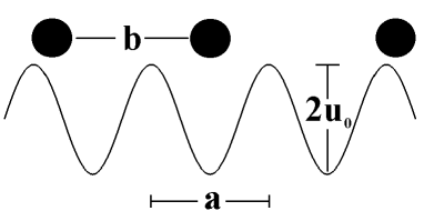
Figure 1: The one-dimensional model

The external force $F$ is applied to every atom in the chain —the total external force is thus $NF$— and $f_{i}$ is a stochastic fluctuating force drawn from a Gaussian distribution, and related to $\eta_{e}$ via the fluctuation-dissipation theorem

$$\left\langle f_{i}(t)\;f_{j}(t)\right\rangle=2\eta_{e}mk_{B}T\delta_{ij}\delta(t)\;,$$ (2)

where $T$ is the temperature of the substrate and $k_{B}$ is the Boltzmann constant. The stochastic force plus the dissipation term provide a thermal bath to describe the otherwise frozen substrate. Moreover, the damping term represents the electronic part of the microscopic friction, which cannot be included in a first principles way in our classical treatment. $\eta_{e}$ may thus be regarded as the electronic sliding friction coefficient. The expression of the interatomic Lennard-Jones potential between adatoms, $V(r)$, where $r=|x_{i}-x_{j}|$, is given by

$$V(r)=\varepsilon\left[\left(\frac{r_{0}}{r}\right)^{12}-2\left(\frac{r_{0}}{r}\right)^{6}\right],$$ (3)

where $r_{0}$ is the $T=0$ equilibrium distance of the dimer and $\varepsilon$ is the depth of the potential well. The interaction is cut-off beyond third neighbors, and hence the cell parameter for the isolated chain is $b=0.9972r_{0}$. The adsorbate-substrate potential $U(x)$ is a periodic potential

$$U(x)=u_{0}\left[\cos\left(2\pi\frac{x}{a}\right)+1\right],$$ (4)

and therefore $a$ is the periodicity of the potential, representing the distance between neighboring substrate atoms; $u_{0}$ is the semi-amplitude of the adsorbate-substrate potential, and it is usually called the substrate corrugation.

In what follows we take $r_{0}$, $\varepsilon$ and the mass $m$ of the adsorbate atoms as the fundamental units of the problem, expressing all other quantities in terms of them. For example, the time unit is $t_{0}=r_{0}\sqrt{m/\varepsilon}$, and consequently in units of $r_{0}=\varepsilon=m=1$ it follows that $t_{0}=1$. As for temperatures they are presented as $k_{B}T$, therefore they are in units of $\varepsilon$.

The periodic boundary conditions impose the following relation between $a$ and $b$:

$$N_{s}a=N_{a}b,$$ (5)

where $N_{s}$ is the number of substrate atoms and $N_{a}$ the number of adsorbed atoms. Therefore, the commensuration ratio between substrate and adsorbate is given by

$$\frac{a}{b}=\frac{N_{a}}{N_{s}}\;.$$ (6)

As was stated the Sec. I, several authors Smith ; Persson96 ; Tomassone97 ; Liebsch99 have already stressed the important role of coverage and corrugation in the understanding of atomic sliding friction. Here we focus on the effect of these parameters, restricting the system to be one-dimensional, in order to avoid any possible topological artifacts that are due to finite size effects. Consequently $a/b$ and $u_{0}$ are our key parameters in the study of the adsorbate-substrate interface response to sliding friction.

Eq. (1) is numerically integrated using a Langevin molecular dynamics algorithm Allen80 ; Allen82 ; Frenkel for 2500 particles ($N_{a}$), with a time step $\Delta t=0.01$. To obtain the friction coefficient $\eta$ an external force $F$ is applied; however, before this force is applied we allow the system to relax during $t_{r}=2500$. Next, $F$ is applied to every adatom, and after another transient period of the same extension the adatoms are presumed to have reached the steady state, with the average friction force equal to the external force (this conjecture is shown below to be valid). Analytically,

$$F=m\eta v\;,$$ (7)

and hence $\eta$ is the effective microscopic friction coefficient which includes the ad hoc friction coefficient $\eta_{e}$ of Eq. (1). In all the calculations presented here we keep the electronic contribution to $\eta$ fixed at $\eta_{e}=5\times 10^{-3}$; as the effective friction coefficient is $\eta=\eta_{e}+\eta_{ph}$, the precise value of $\eta_{e}$ is irrelevant for the calculation of $\eta_{ph}$.

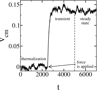
Figure 2: Typical behavior of the adatoms center of mass velocity ($v_{cm}$) during a Langevin molecular dynamics run, before and after the force is applied. In this case $u_{0}=0.04\varepsilon$ and $a/b=0.95$. The applied external force is $F=10^{-3}\varepsilon/r_{0}$ and temperature is $T=0.05\varepsilon/k_{B}$. $v_{cm}$ and $t$ in reduced units of $\sqrt{\varepsilon/m}$ and $r_{0}\sqrt{m/\varepsilon}$ respectively.

Figure 2 shows the typical behavior of the adatoms center of mass velocity during a Langevin molecular dynamics run, before and after the external force is applied. We observe that the system relaxes in a typical time which is less than $1000$ during the thermalization period, and that it enters into a steady state in about the same time after the force is applied. The temperature is $T=0.05$ and the applied force is $F=0.001$. Therefore, in this case, the resulting friction coefficient is $\eta=0.0075$, which implies $\eta_{ph}=0.0025$.

III Results

As was stated above, in this contribution our main concern is the relation between atomic sliding friction and adsorbate-substrate interface topology. Consequently, in this section we present results for our model of the effective sliding friction coefficient $\eta$, for different values of the substrate-adsorbate commensuration ratio $a/b$, and of the substrate corrugation $u_{0}$. We also check on the effect of substrate temperature.

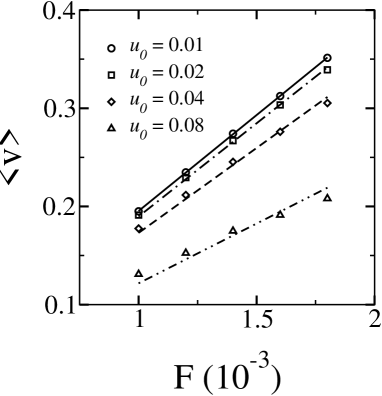
Figure 3: Center of mass velocity $v$ as a function of the external force $F$, in reduced units $[v]=\sqrt{\varepsilon/m}$ and $[F]=\varepsilon/r_{0}$, for four different substrate corrugation values and for a commensuration ratio $a/b=0.451$. The resulting $\eta$ coefficients (in units of $\sqrt{\varepsilon/(mr_{0}^{2})}$) are: $5.12\times 10^{-3}(\bigcirc),5.27\times 10^{-3}(\Box),5.78\times 10^{-3}(\Diamond)$, and $8.22\times 10^{-3}(\bigtriangleup)$.

Once we have made sure that the atomic friction obeys Eq. (7) we obtain from it the effective friction coefficient $\eta$ simply by evaluating the slope of the $F\propto v$ relation. The force $F$ is the input value and the velocity is obtained by time averaging the steady state center of mass velocity, as exemplified for one run in Fig. 2. To obtain reliable data we perform five independent runs for each value of $F$, and we take the average of the resulting $v_{cm}$ values which is denoted as $\langle v_{cm}\rangle$. A set of results for $a/b=0.451$ is shown in Fig 3, where it is observed that, although some deviations are present, the linear relation between $\langle v_{cm}\rangle$ and $F$ is a valid assumption for all the substrate corrugation values considered here. For other commensuration ratios similar pictures are also obtained.

In Figs. 4 we present the results for the effective friction coefficient at $T=0.05$, and for different commensuration ratios. They are separated into two plots, depending on the range of variation of $\eta$ as a function of the corrugation amplitude. Cases where the coefficient $\eta$ rises above $0.9\times 10^{-2}$ at the maximum corrugation amplitude ($u_{0}=0.08$) are shown in Fig. 4(a), while the cases with friction coefficient below that value (at the same corrugation amplitude) are displayed in Fig. 4(b). We denominate them, respectively, “strong” and “weak friction” cases.

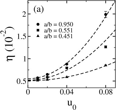
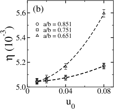
Figure 4: Total friction coefficient (in units of $\sqrt{\varepsilon/(mr_{0}^{2})}$) for a variety of commensuration ratios $a/b$ and for a temperature $T=0.05\varepsilon/k_{B}$. (a) “strong friction” coefficients; (b) “weak friction” coefficients.

Given the theoretical arguments presented by Smith et al. Smith and the numerical evidence presented of Liebsch et al. Liebsch99 , supporting the quadratic dependence of the friction coefficient with substrate corrugation, we fitted the data of Fig. 4 with the following expression:

$$\eta=\eta_{0}+cu_{0}^{2},$$ (8)

where $\eta_{0}$ is the friction coefficient in the absence of corrugation, and thus equal to the “ad-hoc” (or electronic) friction coefficient $\eta_{e}$. The second term of the effective friction coefficient, $cu_{0}^{2}$, is referred to as the phononic friction coefficient, $\eta_{ph}$, which depends quadratically on the corrugation amplitude $u_{0}$. The resulting parabolas can be seen in Fig. 4 (dashed lines) along with the fitted data, while the coefficients $\eta_{0}$ and $c$ are given in Table 1. Notice that our results are consistent with Eq. (8), and that $\eta_{0}$ is indeed equal to $\eta_{e}$.

Table 1: Fitting parameters $\eta_{0}$ and $c$ of Fig. 4

group	$a/b$	$\eta_{0}\;(10^{-3})$		$c\;(10^{-2})$
“strong”	0.451	5.07$\pm$	0.02	52$\pm$	1
	0.551	5.21$\pm$	0.02	139$\pm$	3
	0.950	5.52$\pm$	0.03	217$\pm$	6
“weak”	0.651	5.04$\pm$	0.02	8.6$\pm$	0.5
	0.751	5.04$\pm$	0.01	2.0$\pm$	0.4
	0.851	5.04$\pm$	0.01	2.0$\pm$	0.4

Once it is properly established that the sliding friction (of adsorbate-substrate interfaces) due to phonons depends quadratically on the substrate corrugation amplitude, the coefficient $c$ becomes the main source of information about the phononic friction between different surfaces. A synthesis of the results of the present contribution are given in Fig. 5, where we illustrate the behavior of the coefficient $c$ of Eq. (8) over the whole range of commensuration ratios, and for several different temperature values, using a semi-logarithmic plot. The principal feature of this figure is the region of low $\eta_{ph}$ values for $a/b\approx 0.6-0.9$. Fig. 5(a) and Fig. 5(b) differ on the range of forces used in each one of them. Fig. 5(a) was obtained using forces in the range $0.001-0.002$, while for Fig. 5(b) we used forces in the range $0.0001-0.001$. That the two set of curves are not identical means that the linear assumption for the $f$—$v$ relation is valid only if restricted to relatively small force ranges –less than a decade, as was the case in all previous contributions on sliding friction. We will comment on this below, at the end of this section.

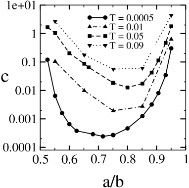
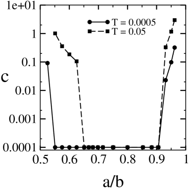
Figure 5: Coefficient $c$ of the phononic friction ($\eta_{ph}=cu_{0}^{2}$) for several commensuration ratios. (a) Results obtained with external force $F$ in the range $0.001-0.002\varepsilon/r_{0}$ and four different temperatures. (b) Results obtained with external force $F$ in the range $0.0001-0.001\varepsilon/r_{0}$ and two different temperatures. The coefficient $c$ is in units of $(mr_{0}^{2}\varepsilon^{3})^{-1/2}$ and temperature is in units of $\varepsilon/k_{B}$.

We conclude from Fig. 5 that the coefficient $c$ has a non-trivial relation with the commensuration ratio, which allows to discriminate between strong and weak phononic friction, i.e. as a function of interface mismatch. Besides, it reflects how the friction coefficient varies with temperature; to illustrate the latter behavior in detail we present in Fig. 6 the relation between $c$ and temperature, for some selected (“strong” cases) values of the commensuration ratio. We see that for a fixed $a/b$ ratio the $c$ coefficient increases linearly with temperature.

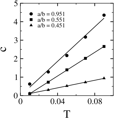
Figure 6: Temperature dependence of the coefficient $c$ for several strong friction commensuration ratio values. The coefficient $c$ is in units of $(mr_{0}^{2}\varepsilon^{3})^{-1/2}$ and temperature is in units of $\varepsilon/k_{B}$.

In order to obtain some insight on the origin of the sliding friction “wide minimum” as a function of commensuration ratio, we look at the adsorbate phonon density of states ${\cal D}(\omega)$, which can be readily computed, in a molecular dynamics simulation, by means of the Fourier transform of the velocity autocorrelation function $\gamma$, given by Dickey69

$$\gamma(t)=\frac{\sum v_{i}(t)\cdot v_{i}(0)}{\sum v_{i}(0)^{2}}\;.$$ (9)

The resulting ${\cal D}(\omega)$ spectra are shown in Figs. 7 for one representative $a/b$ ratio of each group, both at the low temperature $T=0.005$; Fig. 7(a) corresponds to the weak and Fig. 7(b) to the strong friction group. We do so for the $F\neq 0$ (dashed line) and $F=0$ (solid line) steady state cases, where $F$ is the external applied force. Notice that for the strong friction case, extrema of ${\cal D}(\omega)$ in the low frequency region are generated, which closely resemble one-dimensional Van Hove singularities; i.e. points which correspond to extrema (maxima or minima) of the $\omega$ versus $k$ dispersion relation. In our model they are due to the mismatch of the chain and periodic potential periodicities. When the external force is applied an inversion occurs: in the frequency region where there is a minimum for the $F=0$ pre-force situation, a maximum of ${\cal D}(\omega)$ develops during chain sliding. This feature is absent in the weak friction case, where the phonon density of states is much like the typical one for an isolated 1D system, with no difference between the force free ($F=0$) and the driven ($F\neq 0$) cases. As the commensuration ratio $a/b$ crosses over from the strong to the weak friction regime the maxima are quenched.

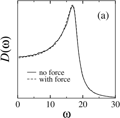
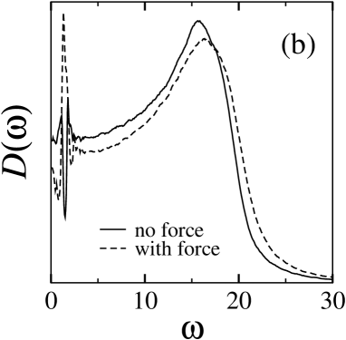
Figure 7: Normalized phonon-frequency spectrum for two different type of commensuration ratio values, one of the (a) weak friction type ($a/b=0.851$) and the other of the (b) strong friction type ($a/b=0.950$) The frequency $\omega$ is presented in units of $\sqrt{\varepsilon/(mr_{0}^{2})}$.

The physical implications of the ${\cal D}(\omega)$ maximum are that in a non-commensurate state some low frequency (large wavelength) modes cannot be excited, since the adsorbate has to adjust to the mismatch condition. However, when the system starts its sliding motion, precisely these ‘soft’ modes are the ones that are excited preferentially, with the consequent amplitude increase in that frequency region. It is just this feature that singles out the most efficient energy dissipation channel. The way in which this is achieved is by pumping center of mass energy into the adsorbate vibration modes that lie in the vicinity of the Van Hove like singularity, which increases the friction relative to the weak friction case, where the mismatch does not impose on the system a frequency region where it does not vibrate ‘comfortably’. Therefore, in the weak friction regime, the phononic dissipation channel is just the usual one.

To provide additional support to this interpretation we plot, in Figs. 8, snapshots of the system as it evolves in time: these snapshots represent the positions of many particles (a section of the chain) as a function of time before and after applying the external force, for strong and weak friction representative cases.

Figures 8(a,b) correspond to a weak friction case, before and after the force is applied, respectively. Figures 8(c,d) are the analogous snapshots for the strong friction case. Comparing Fig. 8(a) and Fig. 8(c) there is an obvious difference between the structure of the chain in equilibrium (without external force), which is due to the constraint imposed by the substrate potential. In the strong case (Fig. 8(c)) the commensuration ratio is such that the system has to significantly rearrange to accommodate to the substrate potential, which is reflected in the kinks that can be observed and which yield a stable pattern. This in turn precludes the system vibrations in a specific collective mode, thus acting as a barrier for the propagation of specific frequencies (as if some modes are pinned) generating the minimum in the density of states of Fig. 7(b). This feature is absent in the snapshot of Fig. 8(a) which can hardly be distinguished from a free chain. So ${\cal D}(\omega)$ looks like a 1D case. When the external force sets the system in sliding motion the kink acts as an excitation, forcing the system to vibrate in what was a forbidden mode for $F=0$. The frozen mode now does slide, as can be seen in Fig. 8(d), where the propagation of the kinks is quite apparent. Therefore, a strong absorption band appears precisely where there was a minimum in the force free situation (Fig. 7(b)). The corresponding weak friction case shows no propagating kink at all and the whole structure is less perturbed (Fig. 7(a)). However, the excitation of all the particles is evident, as for a free chain.

In conclusion, it is our understanding that this could explain the large differences in sliding friction behavior for different commensuration ratios: the key element is the appearance of a new channel of dissipation (due to large wavelength kinks) that is responsible for the increased friction in the strong friction cases. The kink appears when the adsorbate is near perfect commensuration with substrate. This channel acts in parallel with the normal phonon dissipation mechanism.

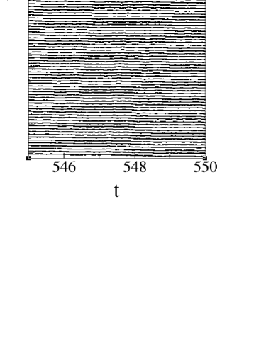
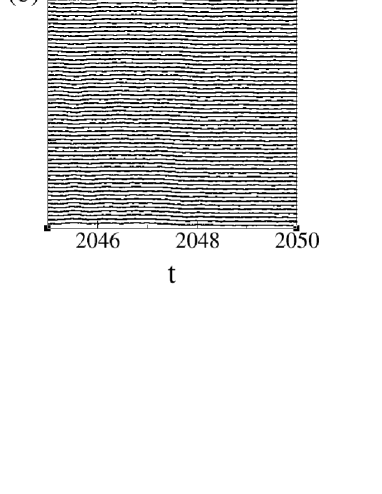
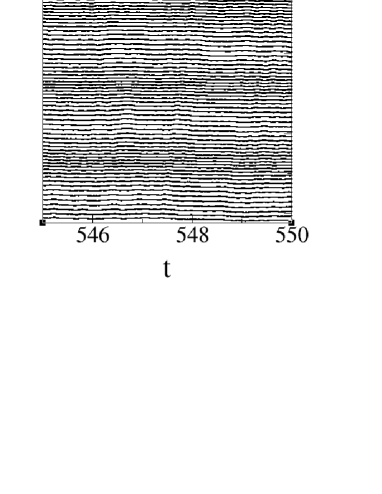
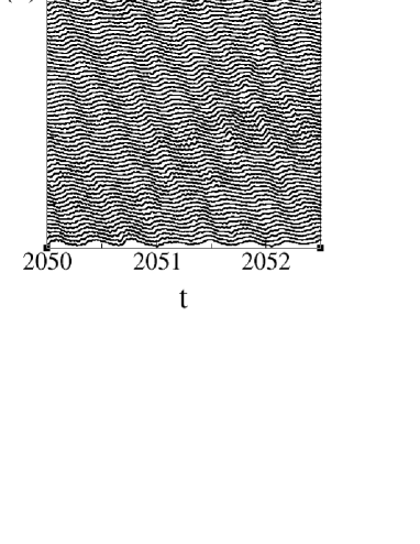
Figure 8: Snapshots of the position of the particles as function of time (in units of $r_{0}\sqrt{m/\varepsilon}$), relative to the center of mass position. In order to emphasizes visualization of the structural change we have diminished the distances between particles. Snaps (a) and (b) correspond to a weak friction case, while snaps (c) and (d) correspond to a strong friction case; snaps (a) and (c) were taken before the application of force, while (b) and (d) were taken after that.

The present results are consistent with those obtained by Braun et al. Braun96 who, using molecular dynamics simulations, studied the mobility and diffusivity of a generalized Frenkel-Kontorova model taking into account anharmonic interactions. In Fig. 9 we compare our results with those of Braun et al. From the definition of mobility it is possible to write

$$B\propto\frac{1}{\eta}\propto\frac{1}{c}$$

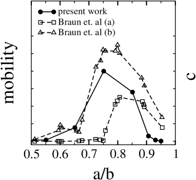
Figure 9: Comparison between our results for the $c$ parameter and Braun et al. data of mobility as a function of commensuration ratio. Present work results are at $k_{B}T=0.01\varepsilon$, while Braun et al. results are at $T=0.0025\;eV$ (a) and $T=0.02\;eV$ (b). Curves (a) and (b) of Braun et al. are curves (1) and (3) respectively of Fig.2 from Ref. Braun96 . The coefficient $c$ is in units of $(mr_{0}^{2}\varepsilon^{3})^{-1/2}$, while mobility is adimensional. The scale was adjusted for the comparison between them.

where $c$ is the proportionality coefficient of Eq. (8). Notice that curve (a) has a maximum for the mobility (minimum for the friction coefficient) in the vicinity of our own maximum, in spite of the different temperatures used in the simulations. In the curve labeled (b), where the difference between temperatures is even larger, the minimum is only slightly shifted to the right. All of the latter points toward the robustness of our interpretation of the enhanced phononic friction.

A final comment: Fig. 5(b) shows the $c$ coefficient —the same that is plotted in Fig. 5(a)— but obtained using a lower range of external forces. If the linear assumption were strictly valid the two graph should be identical; therefore the linear assumption is not generally valid. While this is a very relevant issue, it can be seen that the qualitative general conclusions presented so far are not affected by this. Complementarily, at very low forces  the region of low phononic friction between $0.6-0.9$ are in fact of zero phononic friction, thus only electronic friction should be expected in these cases.

IV Conclusions

A phononic friction coefficient calculation for a one dimensional model of an adsorbate-substrate interface, has been presented. Using molecular dynamics simulations we investigated the system, for different substrate/adsorbate commensuration ratios $a/b$, in order to address two basic questions: first, how the phononic friction (and therefore the sliding friction) depends on the commensuration ratio between substrate and adsorbate; and second, whether a reasonable picture can be found to explain the divergent results between equivalent calculations in the literature Smith ; Persson96 ; Tomassone97 ; Liebsch99 . We believe that both these goals have been attained since, for specific ranges of $a/b$ values, our model calculations yield a relatively large friction coefficient as compared with the intrinsic or electronic friction $\eta_{e}$. This picture holds if $a/b$ falls in what we denominate the strong friction region; otherwise, $\eta_{ph}$ can be neglected in comparison with the electronic friction $\eta_{e}$.

From the technical point of view such sensitive dependence provides a plausible explanation for the divergent results found in the literature Smith ; Persson96 ; Tomassone97 ; Liebsch99 . In fact, a small rotation of the adsorbate relative to the substrate in 2D or 3D simulations of sliding friction, can change the commensuration ratio between the surfaces in such a way as to generate a large change in effective friction, allowing one group to claim that electronic friction is dominant while the other states the opposite, both of them on the basis of properly carried out computations. Our conclusion is that simulations with much larger systems, and averaged over different realizations, have to be performed in order to minimize the artifact imposed by small system simulations or poor averaging. This suggestion implies a rather formidable computational challenge, but certainly more feasible than it was that five or seven year ago.

The present results might appear conflictive when compared with recent results on the friction of a dimer sliding in a periodic substrate Goncalves04 ; Goncalves05 . For the latter system the friction due to vibrations is maximum for a commensuration ratio $a/b=2/3$. However, such a friction is due to resonance of the internal oscillation of the dimer that happens at much higher sliding velocities than the ones used here, since our purpose is to compare to typical experimental setups.

A final question can now be raised: “Is the friction measured in the laboratory sensitive to these subtle changes in the topology, as seen by the sliding layer?” One way to check on this would be to try different adsorbates on the same substrate (for example, comparing Xe, Kr and Ar sliding on Au), or the same adsorbate sliding over different substrates (Xe on Au or Ag).

V Acknowledgments

EST acknowledges the support of CNPq and CAPES. SG acknowledges hospitality of the Department of Physics and Astronomy of the University of New Mexico and support of the National Science Foundation under grants INT-0336343 and DMR-0097204, during the final stages of this work. MK was supported by FONDECyT grant #1030957. This work was supported in part by Fundación Andes.

VI References

References

- (1) J. Krim and A. Widom, Phys. Rev. B38, 12184 (1988).
- (2) E. D. Smith, M. O. Robbins and M. Cieplak, Phys. Rev. B54, 8252 (1996).
- (3) B. N. Persson and A. Nitzan, Surf. Sci. 367, 261 (1996).
- (4) M. S. Tomassone, J. B. Sokoloff, A. Widom and J. Krim, Phys. Rev. Lett. 79, 4798 (1997).
- (5) A. Liebsch, S. Gonçalves and M. Kiwi, Phys. Rev. B60, 5034 (1999).
- (6) M. O. Robbins and M. H. Müser, Computer Simulations of Friction, Lubrication and Wear, in Modern Tribology Handbook, (Edited by B. Bhushan, CRC Press, Boca Raton, 2001), pp. 717-765, and references cited therein.
- (7) M. H. Müser, L. Wenning and M. O. Robbins, Phys. Rev. Lett. 86, 1295 (2001).
- (8) C. Daly and J. Krim, Phys. Rev. Lett. 76, 803 (1996).
- (9) A. Dayo, W. Alnasrallah and J. Krim, Phys. Rev. Lett. 80, 1690 (1998).
- (10) M. P. Allen, Mol. Phys. 40, 1073 (1980).
- (11) M. P. Allen, Mol. Phys. 47, 599 (1982).
- (12) D. Frenkel and B. Smit, Understanding Molecular Simulation, (Academic Press, San Diego, California, 1996).
- (13) J. M. Dickey and A. Paskin, Phys. Rev. 188, 1407 (1969).
- (14) O. M. Braun, T. Dauxois, M. V. Paliy and M. Peyrard, Phys. Rev. B54, 321 (1996).
- (15) S. Gonçalves, V. M. Kenkre and A. R. Bishop, Phys. Rev. B 70, 195415 (2004).
- (16) S. Gonçalves, C. Fusco, A. R. Bishop and V. M. Kenkre, cond-mat/0503725.