Quantum phase transition and sliding Luttinger liquid in coupled $t-J$ chains

Abstract

Using a recently proposed perturbative numerical renormalization-group algorithm, we explore the connection between quantum criticality and the emergence of Luttinger liquid physics in $t-J$ chains coupled by frustrated interactions. This study is built on an earlier finding that at the maximally frustrated point, the ground state of weakly-coupled Heisenberg chains is disordered, the transverse exchanges being irrelevant. This result is extended here to transverse couplings up to $J_{\perp}=0.6$, and we argue that it may also be valid at the isotropic point. A finite size analysis of coupled Heisenberg chains in the vicinity of the maximally frustrated point confirms that the transverse spin-spin correlations decay exponentially while the longitudinal ones revert to those of decoupled chains. We find that this behavior persists upon moderate hole doping $x\lesssim 0.75$. For larger doping, the frustration becomes inactive and the quantum critical point is suppressed.

I Introduction

In a number of materials including cuprate high temperature superconductors reviewHTC , organic reviewOC and inorganic reviewIOC quasi one-dimensional (1D) conductors, the physics is dominated by the combined effect of low dimensionality, strong electron correlations and competing orders. These materials display a phenomenology, in the metallic state above the ordered states, which departs from the Fermi liquid (FL) picture. This has motivated a search for a new paradigm which goes beyond FL theory. Two new ideas, electron fractionalization anderson ; kivelson0 and quantum criticality sachdev (QC), have been proposed as the possible physical effects which may lead to the observed non-FL behavior.

The breakdown of the FL theory is known to occur in 1D where the low energy physics is described by Luttinger liquid (LL) theory. The LL is fundamentally different from a FL; for instance, instead of the quasiparticle peak displayed by the FL at zero energy in the spectral weight function, a pseudogap is observed in the LL. This is because in the LL the low energy excitations are collective spin density and charge density, in contrast to the FL where they are still electron-like. An interpretation of this phenomenon is that the electron fragments into density waves known as spinons and holons which propagate with different velocities. The LL would thus be the natural starting point to search for non-FL behavior in higher dimension. However, it has been impossible to find a LL in dimensions greater than one using perturbative methods. This has been tried by starting from 1D models coupled by a small transverse hopping bourbonnais or directly from the 2D non-interacting electron gas in which the interaction is introduced perturbativelyshankar . It was found in both cases that the FL is the stable fixed point. An alternative strategy applied recently is to build a LL fixed point in anisotropic 2D systems by coupling 1D LLs by marginal transverse strong forward density-density or current-current couplings kivelson ; carpentier ; kane . The new 2D fixed point, called sliding LL (SLL), retains the physics of the 1D LL. It was shown that there is a regime of parameters in which Josephson, charge and spin density waves and single particle hopping are irrelevant, i.e., a domain of stability of the 2D LL. There has not been, to the author’s knowledge, any detailed analysis as to why these two approaches lead to conflicting conclusions. It would appear that using simple perturbation theory, one cannot go smoothly from a single chain to a SLL.

A different approach has been to assign the departure from a FL behavior to the proximity of a quantum critical point (QCP)sachdev . Because of the proximity of the QCP the adiabatic continuity concept, which is the basis of the FL theory, is no longer valid. In the normal state, the eigenstates of the system are a mixture of states which evolve separately into the ground states existing on the two sides of the QCP. Because of this mixture, the single-particles excitations of the system are not simple electron-like excitations as in the FL.

Considering the pure spin one-half limit of the problem, various studies have found that any small exchange leads to the onset of long-range order. Laughlin laughlin has argued that spin-$1/2$ systems have the propensity to order and it is only at a QCP that they do not. Yet considering that experiments clearly show a departure from the FL, one can still retain the electron fractionalization hypothesis as the driving mechanism of the non-FL but attribute it not to LL physics but to the presence of a QCP. This suggests that in constructing a model Hamiltonian for coupled LLs, one must include competing interactions that preclude any order at the QCP.

The difference between the SLL and QCP physics is ultimately two different views of the same reality. If they are both correct, they should emerge from a well controlled study of an appropriate microscopic Hamiltonian. The two-step density-matrix renormalization group (TSDMRG) moukouri-TSDMRG ; moukouri-TSDMRG2 offers a new approach to study these issues. Although it is a perturbative approach, it has the important non-perturbative property that it can lead to an ordered state starting from a disordered statemoukouri-TSDMRG2 ; moukouri-KB . Thus it has the ability to treat effectively the different ground states that may arise in weakly coupled chains.

In this paper, we apply the TSDMRG to study the QPT in the spatially anisotropic $t-J-t_{\perp}-J_{\perp}-J_{d}$ model. We show that in this model the concept of LL can be unified with that of quantum criticality, namely that the model undergoes a QPT at $J_{d}=J_{\perp}/2$ (These couplings are defined in the Hamiltonian ( 1) given below). At the QCP the system is in a state made of nearly disconnected chains that can be interpreted as a SLL. We first analyze the half-filling case which corresponds to the anisotropic $J_{1}-J_{2}$ model. We show that the dimerization found in previous approximate field theory analyses tsvelik ; starykh does not occur. We then study the doped case at hole densities up to $x=0.4$. The picture observed in the half-filled case remains valid at moderate dopings. At the QCP, the transverse spin-spin correlation function decays exponentially as in the half-filled case. But at higher dopings, the frustration becomes ineffective and the transition is suppressed; the ground state is a spin density wave at all couplings. This suggests the existence of a SLL to FL crossover at finite temperature.

II Model and Method

The anisotropic $t-J-t_{\perp}-J_{\perp}-J_{d}$ model is:

$$H=-t\sum_{i,l}(c_{i,l}^{\dagger}c_{i+1,l}+h.c.)+J\sum_{i,l}{\bf S}_{i,l}{\bf S}_{i+1,l}-\frac{1}{4}n_{i,l}n_{i+1,l}$$

$$-t_{\perp}\sum_{i,l}(c_{i,l}^{\dagger}c_{i,l+1}+h.c.)+J_{\perp}\sum_{i,l}{\bf S}_{i,l}{\bf S}_{i,l+1}-\frac{1}{4}n_{i,l}n_{i,l+1}$$

$$+J_{d}\sum_{i,l}{\bf S}_{i,l}{\bf S}_{i+1,l+1}+{\bf S}_{i+1,l}{\bf S}_{i,l+1}$$ (1)

where $t$ and $J>0$ are the in-chain hopping and exchange parameters; $t_{\perp}$ and $J_{\perp}>0$ are the transverse hopping and exchange parameters; $J_{d}>0$ is the diagonal exchange parameter. We start by describing the extension to fermion systems of the numerical renormalization method, which has been applied so far only to spin systems moukouri-TSDMRG ; moukouri-TSDMRG2 . There is no significant difficulty in going from spins to fermions. One should simply be careful to consistently apply fermion anticommutation rules. It is crucial to choose an order for the sites in the 2D lattice and keep it throughout the derivation of the algorithm. The method is a special case of a more general matrix perturbation method based on the Kato-Bloch expansion kato ; bloch which was recently introduced by the author moukouri-KB . The method has two main steps. In the first step, the usual 1D DMRG method white is applied to find a set of low lying eigenvalues $\epsilon_{n}$ and eigenfunctions $|\phi_{n}\rangle$ of a single chain. In the second step, the 2D Hamiltonian is then projected onto the basis constructed from the tensor product of the $|\phi_{n}\rangle$’s. This projection yields an effective one-dimensional Hamiltonian for the 2D lattice,

$$\tilde{H}\approx\sum_{[n]}E_{\parallel[n]}|\Phi_{\parallel[n]}\rangle\langle\Phi_{\parallel[n]}|-t_{\perp}\sum_{i,l}(\tilde{c}_{i,l}^{\dagger}\tilde{c}_{i,l+1}+h.c.)+$$

$$J_{\perp}\sum_{il}{\bf\tilde{S}}_{i,l}{\bf\tilde{S}}_{i,l+1}-\frac{1}{4}\tilde{n}_{i,l}\tilde{n}_{i+1,l}$$

$$J_{d}\sum_{il}{\bf\tilde{S}}_{i,l}{\bf\tilde{S}}_{i+1,l+1}+{\bf\tilde{S}}_{i+1,l}{\bf\tilde{S}}_{i,l+1},$$ (2)

where $E_{\parallel[n]}$ is the sum of eigenvalues of the different chains, $E_{\parallel[n]}=\sum_{l}{\epsilon_{n_{l}}}$; $|\Phi_{\parallel[n]}\rangle$ are the corresponding eigenstates, $|\Phi_{\parallel[n]}\rangle=|\phi_{n_{1}}\rangle|\phi_{n_{2}}\rangle...|\phi_{n_{L}}\rangle$; $\tilde{c}_{i,l}^{\dagger}$, $\tilde{c}_{i,l}$, and ${\bf\tilde{S}}_{i,l}$ are the renormalized matrix elements in the single chain basis. They are given by

$$(\tilde{c}_{i,l}^{\dagger})^{n_{l},m_{l}}=(-1)^{n_{i}}\langle\phi_{n_{l}}|{c}_{i,l}^{\dagger}|\phi_{m_{l}}\rangle,$$ (3)

$$(\tilde{c}_{i,l})^{n_{l},m_{l}}=(-1)^{n_{i}}\langle\phi_{n_{l}}|{c}_{i,l}|\phi_{m_{l}}\rangle,$$ (4)

$${\bf\tilde{S}}_{i,l}^{n_{l},m_{l}}=\langle\phi_{n_{l}}|{\bf S}_{i,l}|\phi_{m_{l}}\rangle,$$ (5)

where $n_{i}$ represents the total number of fermions from sites $1$ to $i-1$. For each chain, operators for all the sites are stored in a single matrix

$$\tilde{c}_{l}^{\dagger}=(\tilde{c}_{1,l}^{\dagger},...,\tilde{c}_{L,l}^{\dagger}),$$ (6)

$$\tilde{c}_{l}=(\tilde{c}_{1,l},...,\tilde{c}_{L,l}),$$ (7)

$${\bf\tilde{S}}_{l}=({\bf\tilde{S}}_{1,l},...,{\bf\tilde{S}}_{L,l}).$$ (8)

Since the in-chain degrees of freedom have been integrated out, the interchain couplings are between the block matrix operators in Eq.( 6, 7, 8) which depend only on the chain index $l$. In this matrix notation, the effective Hamiltonian is one-dimensional and it is also studied by the DMRG method. The only difference with a normal 1D situation is that the local operators are now $m\times m$ matrices, where $m$ is the number of states kept to describe the single chain. In this study, mostly exact diagonalization (ED) instead of DMRG is used in the 1D part of the algorithm. This has the obvious advantage that all the eigenvectors and eigenvalues are known up to a well defined accuracy which is set to $10^{-6}$ in the Davidson algorithm used to obtain them. The two-step DMRG method is variational moukouri-TSDMRG2 ; alvarez , so the results can systematically be improved by increasing $m$. In this study, the calculations were done on a Dell 670 dual Xeon (3.4 GHz) workstation with 4GB of RAM. The maximum $m$ we can reach for the calculations to run within a reasonable time (about three days) is about $m=96$ for a $L\times(L+1)$ lattice with $L=16$.

In this study, we are mostly concerned with the parameter regime where $J_{d}\approx J_{\perp}/2$. It is in this regime that the sign problem in the QMC is the most severe. In Ref.alvarez , we have shown that the two-step DMRG is at its best in the highly frustrated regime where QMC simulations cannot be done. To illustrate this fact, we show in Table( 1) the ground state energy ($E_{G}$) as a function of $m$ for the unfrustrated case, with $J_{\perp}=0.2$ and $J_{d}=0$, and in the frustrated case at the maximally frustrated point ( this point is defined below), with $J_{\perp}=0.2$ and $J_{d}=0.114$, for a $12\times 13$ lattice. The extrapolated value of $E_{G}$ in the unfrustrated case is in good agreement with the QMC. It can be seen that $E_{G}$ converges faster in the frustrated case. The strategy in this study is to increase $J_{\perp}$ while the ratio $J_{d}/J_{\perp}$ remains close to $0.5$. We do not expect a significant decrease in accuracy for larger $J_{\perp}$ because as we will see below, the interchain correlations decay exponentially in this region. Thus despite its perturbative nature, the TSDMRG is able to treat model( 1) well beyond the weak coupling regime as long as one stays in the vicinity of the QCP.

$m/J_{d}$	$0.$	$0.114$
$32$	0.43796	0.42898
$64$	0.43928	0.42917
$96$	0.43970	0.42920
$\infty$	0.44051	0.42921
QMC	0.44075

Table 1: Ground-state energies as function of $m$ and $J_{d}$ for $J_{\perp}=0.2$.

The high accuracy enjoyed at half-filling is somewhat reduced in the doped case. The reason behind this reduction is simply that the size of the total Hilbert space increases as one goes from two degrees of freedom per site to three. Since we keep roughly the same number of states in the two cases, the accuracy will be smaller for doped systems. This can be seen, for instance, when $m=96$ states are kept in the second step. The energy width of the retained states drops from $\Delta E\approx 1.6$ at half-filling to $\Delta E\approx 0.8$ when the doping is $x=0.125$ for a $L=16$ system. Another difficulty which arises upon doping is that one needs to target, during the first step of the algorithm, at least three charge sectors in order to keep matrix elements which involve interchain hopping. A typical situation is $L=16$ and $x=0.125$, where the corresponding ground state has $14$ electrons. For this charge sector, five spin sectors with $S_{Z}=0,\pm 1,\pm 2$ were targeted. For charge sectors with $13$ and $15$ electrons, four spin sectors with $S_{Z}=\pm 0.5,\pm 1.5$ were also targeted. Unlike the half-filled case, ED was not done for all doped systems in the first step. For instance for $L=16$, we kept $243$ states. This number of states corresponds to an exact diagonalization of 12 sites which means three DMRG iterations were necessary to reach the desired size. Hence, the truncation error at the end of the first step increases from zero at half-filling to about $1\times 10^{-6}$ in the doped case.

Removing or adding one electron on a finite system can significantly affect the density if the system size is not large enough. For instance, during the study of a $L=16$ lattice with the hole density $x=0.125$, the nominal ground state has 14 electrons, whereas the ground states with 13 and 15 electrons correspond to the hole densitites $0.1875$ and $0.0625$ respectively. Thus, adding or removing holes on small systems induces large variations of the hole density, resulting in large differences between the ground states of the different charge sectors. These variations are the largest near half-filling for small values of $J$. As a consequence, the electrons cannot jump between the chains and the charge degrees of freedom remain decoupled for small values of the interchain hopping. It is necessary to fine tune $J$ so that these energy differences are smaller or of the same magnitude as $t_{\perp}$. For $t_{\perp}=0.2$, which will be used for all doped systems, $J$ was chosen so that the difference $\delta_{c}$ between ground state energy of charge sectors differing by one electron is such that $\delta_{c}\lesssim 0.16$. Fixing $\delta_{c}$ amounts to fixing the chemical potential instead of the coupling. The value of $J$ which satisfies this criterion depends on the hole density $x$. These values are listed in Table 2 for $L=16$ systems.

$x$	$0.125$	$0.25$	$0.375$
$J$	1.4	1.14	0.75
$E(N)-E(N+1)$	0.1012	0.0982	0.1355
$E(N)-E(N-1)$	0.1250	0.1658	0.1615

Table 2: Hole densities, corresponding exchange couplings and energy differences between charge sectors for $L=16$.

III Finite size analysis at the critical point at half-filling

The half-filled case corresponds to weakly coupled Heisenberg chains that we studied in Refmoukouri-TSDMRG2 . In that study it was found that the model displays two phases: a Néel $Q=(\pi,\pi)$ when $J_{d}/J_{\perp}\lesssim 0.5$ and a Néel $Q=(\pi,0)$ when $J_{d}/J_{\perp}\gtrsim 0.5$. These two phases are separated by a critical point where the long-distance behavior of the spin-spin correlations along the chains in the 2D system is identical to those in the disconnected chains. In this study, we will show that this behavior found for small $J_{\perp}\lesssim 0.2$ extends well beyond the weak interchain coupling regime (up to $J_{\perp}=0.6$). The nature of the ground state in this regime, which was previously called ”nearly independent chains”, will be further clarified by the analysis of the interchain spin-spin correlations. Before starting the finite size analysis, it is important to stress the fact that the open boundary conditions (OBC) which were applied in most of this study create some difficulty in the interpretation of data. While OBC have the advantage of yielding higher accuracy in DMRG simulations, they artificially break the lattice translational symmetry. The OBC thus introduce a spurious dimerization $d$ in the 1D chain, as we will see below, which converges very slowly toward zero. To our knowledge, the exact behavior of this dimerization as a function of the system size has not been reported in the literature. On top of this difficulty, one must account for logarithmic corrections to the finite size quantities. For instance, fitting $d$ with $1/L$, one finds that $d$ extrapolates to a finite value in the limit $L\rightarrow\infty$. This deviation from $0$, which is the true limit, is the signature of logarithmic corrections. Logarithmic corrections in an open Heisenberg chain have been studied in Ref. affleck . They are due to marginally irrelevant operators and their mathematical form is hard to find exactly for small systems. A functional form exists only in the limit of large $L$. For instance, the finite size spin gap has the following form

$$\Delta_{L}\approx\frac{\pi v}{L}[1-\frac{4\pi g(L)}{\sqrt{3}}]$$ (9)

where $v=\pi/2$ is the spin velocity and $g(L)$ a function such that

$$g(L)\rightarrow\frac{\sqrt{3}}{4\pi\log{L}}$$ (10)

when $L$ is very large. For small chains, $g(L)$ has to be introduced as an unknown parameter which is obtained by fitting the data to known limits. Since the main interest of this study lies in the relative behavior of the 2D system with respect to an isolated 1D chain, we will not use $g(L)$ during the finite size analysis. When performing the finite size analysis, simple linear or quadratic functions of $1/L$ will be used even though they do not lead to the exact values in the thermodynamic limit for the 1D system because of the logarithmic corrections.

III.1 Ground-state energies

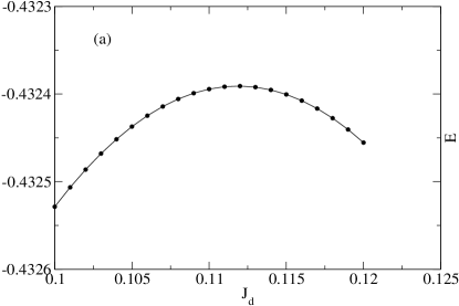
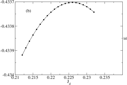
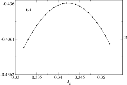
Figure 1: Ground-state energies for $L=16$ and $J_{\perp}=0.2$(a), $J_{\perp}=0.4$ (b) and, $J_{\perp}=0.6$ (c) as function of $J_{d}$.

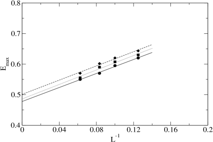
Figure 2: Maxima of the ground-state energies as function of the lattice size for $J_{\perp}=0.2$ (circles), $J_{\perp}=0.4$ (squares) and, $J_{\perp}=0.6$ (diamonds).

$J_{\perp}$	$L=8$	$L=10$	$L=12$	$L=16$
$0.2$	0.124	0.119	0.114	0.112
$0.4$	0.252	0.243	0.236	0.226
$0.6$	0.386	0.372	0.361	0.342

Table 3: Values of $J_{d}$ corresponding to the maximum of the ground-state energy for different $J_{\perp}$ and $L$.

The ground-state energies shown in Fig.( 1) show similar behavior for all values of $J_{\perp}$ when $J_{d}$ is varied. Starting from $J_{d}=0$ where the ground state is a Néel $Q=(\pi,\pi)$ phase, $E_{G}$ typically increases with $J_{d}$ until it reaches a maximum, labeled the maximally frustrated point $J_{d}^{max}$. Then $E_{G}$ decreases when $J_{d}>J_{d}^{max}$ where the ground state is in a Néel $Q=(\pi,0)$ phase. The ratio $J_{d}^{max}/J_{\perp}$ depends on both $J_{\perp}$ and $L$. For small $J_{\perp}$, $J_{d}^{max}/J_{\perp}$ remains very close to $0.5$ but deviates from this value as $J_{\perp}$ increases. Previous studies ( see Ref.lhuillier for a review) found $J_{d}^{max}/J_{\perp}=0.6$ when $J_{\perp}=1$. This deviation is larger for OBC than for PBC. This is because the maximally frustrated point corresponds to the point where the transverse component of the Fourier transform of the coupling

$$J(Q)=2\cos{Q_{x}}+2\cos{Q_{y}}[J_{\perp}+2J_{d}\cos{Q_{x}}]$$ (11)

vanishes when $Q_{x}=\pi$. At this point $2J_{d}$ bonds cancel one $J_{\perp}$ bond. But when OBC are used on a $L\times(L+1)$ lattice, one has $L^{2}$ bonds but only $2L(L-1)$ $J_{d}$ bonds. Thus for small lattices, there is a deficit in $J_{d}$ bonds which translates into the shift of the maximum towards larger $J_{d}$ for a fixed $J_{\perp}$.

This shift has been argued to be indicative of the existence of an intermediate phase, possibly dimerized, in the region between $J_{d}=0.4$ (where the Néel $Q=(\pi,\pi)$ order parameter was found to vanish) and $J_{d}=0.6$ (where the Néel order parameter $Q=(\pi,0)$ or $(0,\pi)$ vanishes). Our results shown in Table( 3), which list the position of the maxima for various $J_{\perp}$ and $L$, indicate that this deviation of $J_{d}^{max}/J_{\perp}$ from $0.5$ is simply a finite size effect. For a fixed $L$, $J_{d}^{max}/J_{\perp}$ increases with $J_{\perp}$ in agreement with the finding in the isotropic case. But one can see that for a fixed $J_{\perp}$, $J_{d}^{max}/J_{\perp}$ decreases with $L$. Fig.( 2) displays the extrapolated values of $J_{d}^{max}/J_{\perp}$ for $J_{\perp}=0.2$, $0.4$, and $0.6$. They all converge to the vicinity of $0.5$. Aside from numerical uncertainties, it is thus likely that $J_{d}^{max}/J_{\perp}=0.5$ for all $J_{\perp}$ in the thermodynamic limit.

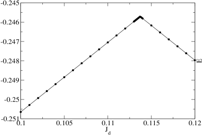
Figure 3: Ground-state energies for $L=16$ and $J_{z\perp}=0.2$ in the Ising case.

The curves of $E_{G}$ in Fig.( 1) show that $E_{G}$ is differentiable, which suggests that the transition could be of second order. This is to be constrasted with the pure Ising equivalent of Hamiltonian ( 1) obtained by setting all XY terms to $0.$ $E_{G}$ for the Ising case shown in Fig.( 3) is not differentiable at $J_{d}^{max}/J_{\perp}$, as expected since this transition is of first order. It is to be noted that in this case where quantum fluctuations are absent, $J_{d}^{max}/J_{\perp}$ does not occur at $0.5$. This is another fact which favors the conclusion that the deviation from $0.5$ seen in previous studies sindzingre is a finite size effect rather than some subtle quantum effect due to the existence of an intermediate phase between the two Néel ordered states.

III.2 Short-distance spin-spin correlations

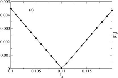
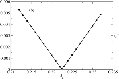
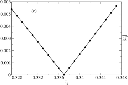
Figure 4: $C_{1}$ for $L=16$ and $J_{\perp}=0.2$(a), $J_{\perp}=0.4$ (b) and, $J_{\perp}=0.6$(c) as function of $J_{d}$.

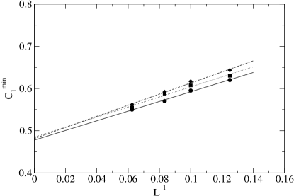
Figure 5: Minima of $C_{1}$ as function of the lattice size for $J_{\perp}=0.2$ (circles), $J_{\perp}=0.4$ (squares) and, $J_{\perp}=0.6$ (diamonds).

$J_{\perp}$	$L=8$	$L=10$	$L=12$	$L=16$
$0.2$	0.124	0.119	0.114	0.110
$0.4$	0.252	0.243	0.235	0.222
$0.6$	0.386	0.372	0.359	0.337

Table 4: Values of $J_{d}$ corresponding to the minimum of $C_{1}$ for different $J_{\perp}$ and $L$.

The first neighbor transverse correlation function (Fig.( 4))

$$C_{1}=\langle S_{il}^{z}S_{il+1}^{z}\rangle$$ (12)

taken in the middle of the lattice $(il)=(L/2,L/2+1)$ is linear in the vicinity of $J_{d}^{max}/J_{\perp}$ and vanishes at the minimum point $J_{d}^{0}$. Table( 4) lists the position of $J_{d}^{0}$ for various $J_{\perp}$ and $L$. These values of $J_{d}^{0}$ are equal to or near $J_{d}^{max}$ found for $E_{G}$ for all values of $J_{\perp}$ studied. We believe that the small differences between the values of $J_{d}^{0}$ and $J_{d}^{max}$ are due to numerical errors on $C_{1}$ and $E_{G}$. The difference between these positions are in all cases less than $0.1\%$. Since the DMRG technique tends to have a better accuracy on the ground-state energies than on the correlation functions, the position of the maximum in $E_{G}$ is taken as the reference for the transition. The position of the minimum shown in Fig.( 5) extrapolate as for $E_{G}$ towards $J_{d}/J_{\perp}=0.5$.

Since $C_{1}=0$ at the transition point, the spins in different chains remain uncorrelated as in the classical case. This is indeed the best way to minimize frustration. In order to avoid the cost in energy induced by frustrated bonds, the system forms the largest unfrustrated cluster allowable. In this case, the largest unfrustrated clusters are independent chains. This state can actually be seen as the generalization of the Majumdar-Gosh state known in 1D systems lhuillier . However, this does not mean that the chains are completely disconnected as in the classical case. In the results on $E_{G}$ above we were unable to find a point in the parameter space where the ground-state energy of the coupled 2D system is exactly equal to the ground-state energy of disconnected chains. The ground state energies of the 2D systems are always lower than that of completely disconnected chains. This means that despite the fact that $C_{1}=0$, all other transverse correlations are not necessarily zero at $J_{d}=J_{d}^{0}$ as in the classical case.

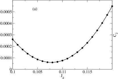
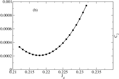
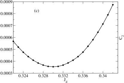
Figure 6: $C_{2}$ for $L=16$ and $J_{\perp}=0.2$(a), $J_{\perp}=0.4$ (b) and, $J_{\perp}=0.6$ (c) as function of $J_{d}$.

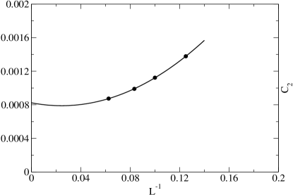
Figure 7: Value of $C_{2}$ at the minimum as function of the lattice size for $J_{\perp}=0.6$ (circles).

The second neighbor correlation

$$C_{2}=\langle S_{il}^{z}S_{il+2}^{z}\rangle$$ (13)

shown in Fig.( 6), taken at $(il)=(L/2,L/2+2)$, does not vanish. It instead has a minimum at $J_{d}^{min}$ for all values of $J_{\perp}$. The values of $C_{2}$ corresponding to $J_{d}=J_{d}^{0}$ shown in Fig.( 7) for $J_{\perp}=0.6$ extrapolate to a finite value in the thermodynamic limit. Thus, at the point where $C_{1}=0$, $C_{2}$ has a small finite value. It is worth noting that the dimerization is not the only way to avoid frustration as it is commonly believed lhuillier .

III.3 Dimerization

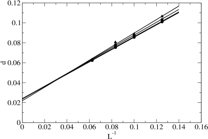
Figure 8: Evolution of the dimerization as function of the lattice size for $J_{\perp}=0.$ (circles), $J_{\perp}=0.2$ (squares), $J_{\perp}=0.4$ (diamonds) and, $J_{\perp}=0.6$ (triangles).

The examination of the short-range correlations above proves that at the maximally frustrated point, there is a weak bond between the chains. The ground-state in this region of parameters has been predicted via field theoretic approaches tsvelik ; starykh to be a columnar dimer state, with the dimerization occuring along the chains. In order to see if dimerization occurs along the chains, we compute the quantity

$$d_{il}=\langle S_{2il}^{z}S_{2i+1l}^{z}\rangle-\langle S_{2i+1l}^{z}S_{2i+2l}^{z}\rangle.$$ (14)

One should note that since we use the OBC, we are in the most favorable situation for the dimerization. i.e., the OBC breaks the translational symmetry of the chains and even isolated finite chains are dimerized. This spurious dimerization decays very slowly as $L\rightarrow\infty$. It is thus expected that if indeed the system dimerizes at the QCP, the finite size behavior of $d_{il}$ of the coupled system will be different from that of isolated chains. In Fig.( 8) $d$ is shown for $J_{\perp}=0$, $0.2$, $0.4$, and $0.6$ and for various sizes at $J_{d}^{max}$ in the relevant cases. $d$ converges to the same limit whether $J_{\perp}=0$ or not. Since the single chain is not dimerized, this shows that the 2D system at the critical point is not dimerized either.

We are aware of a different conclusion reached by a recent bosonization approach coupled to a renormalization group and mean-field analyses starykh . In that study for a two-leg ladder in the vicinity of the maximally frustrated point, it was found that although the action of $J_{\perp}$ is largely cancelled by $J_{d}$, at the second order there remains residual couplings ${\tilde{J}}_{1}=2J_{d}^{2}/\pi^{2}$ and ${\tilde{J}}_{2}=-3J_{d}^{2}/\pi^{2}$ which are relevant. ${\tilde{J}}_{1}$ favors Néel order and ${\tilde{J}}_{2}$, the ring-exchange term, favors a dimerized state. These authors then carried out a self-consistent mean-field approximation of the competition between ${\tilde{J}}_{1}$ and ${\tilde{J}}_{2}$ in the 2D system. They found a narrow dimerized state between the two ordered magnetic states. According to their conclusions, our prediction of the spin liquid state at the transition is due to finite size effects. But our results above, performed for larger interchain couplings for which the dimerization should be more apparent and is not seen, rather support our conclusions in Ref. moukouri-TSDMRG2 . There is additional evidence, discussed below, obtained from the study of the three-leg ladderwang which also agrees with the absence a dimer phase. It is important mentioning that this type of RG analysis is not without a certain bias. The RG transformation usually leads to a proliferation of couplings. There is often some degree of arbitrariness in the choice of the relevant couplings.

III.4 Long-distance spin-spin correlations

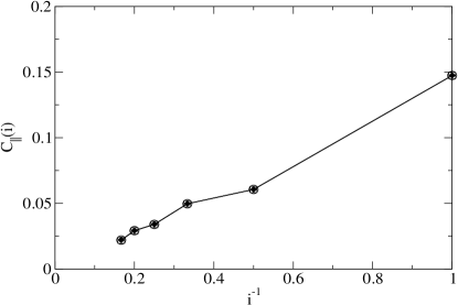
Figure 9: Longitudinal spin-spin correlation at $J_{d}^{max}$ as function of the distance for $L=16$ and, $m=32$ (circles), $m=64$ (squares) and, $m=96$ (diamonds).

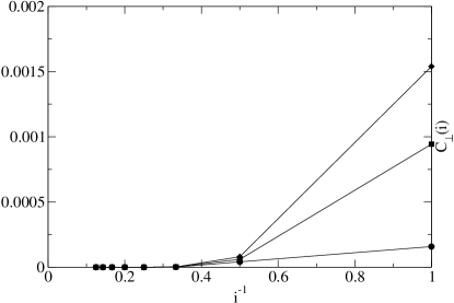
Figure 10: Transverse spin-spin correlation at $J_{d}^{max}$ as function of the distance for $L=16$ and, $m=32$ (circles), $m=64$ (squares) and, $m=96$ (diamonds).

Near the maximally frustrated point, the long distance behavior of the in-chain spin-spin correlation functions is nearly identical to that of the disconnected chains. These correlations shown in Fig.( 9) for $J_{\perp}=0.2$ and $L=16$ are nearly independent of $m$. This is because, for a purely 1D system of this size they are already known with very good accuracy. Since the chains are nearly disconnected, no significant increase of $m$ is required to describe them with the same level of accuracy as in 1D.

This conclusion is supported by the behavior of the transverse correlation functions shown in Fig.( 10) for the same set of parameters. $C_{\perp}(i)$ is found to be equal to $0$ for $i\gtrsim 4$ for all the values of $m$.

$C_{\parallel}(i)$ and $C_{\perp}(i)$ are independent of $J_{\perp}$ at the maximally frustrated point, i.e. only the ratio $J_{d}/J_{\perp}$ is important up to intermediate values. This is seen in Fig.( 11) and Fig.( 12) where these quantities are compared for $J_{\perp}=0.2$, $0.4$ and $0.6$. $C_{\parallel}(i)$ is nearly identical to that of independent chains while $C_{\perp}(i)$ remains very small and decays exponentially with $i$. This behavior is valid from weak to intermediate coupling regimes. It is to be noted that since the maximally frustrated point is chosen at the maximum $J_{d}^{max}$ of $E_{G}$, $C_{1}$ is not equal to $0$ because the two quantities differ slightly as shown in Table( 3, 4) because of numerical uncertainties.

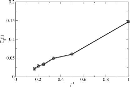
Figure 11: Longitudinal spin-spin correlation at $J_{d}^{max}$ as function of the distance for $J_{\perp}=0.$ (circles), $J_{\perp}=0.2$ (squares), $J_{\perp}=0.4$ (diamonds) and, $J_{\perp}=0.6$ (triangles).

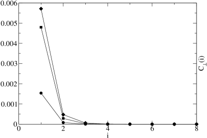
Figure 12: Transverse spin-spin correlation at $J_{d}^{max}$ as function of the distance for $J_{\perp}=0.2$ (circles), $J_{\perp}=0.4$ (squares) and, $J_{\perp}=0.6$ (diamonds).

This behavior of $C_{\perp}(i)$ at $J_{d}\approx J_{\perp}/2$ is to be contrasted to that of the magnetic regime. In Fig.( 13) we see that for instance, $C_{\perp}(4)$ of the magnetic case is already four orders of magnitude larger than in the disordered case. The exponential decay of $C_{\perp}(i)$ seen in Fig.( 13) and the decay of $C_{\parallel}(i)$ which is nearly that of decoupled chains suggest that for $J_{d}\approx J_{\perp}/2$, the system displays a spin analog of the sliding Luttinger liquid (SLL) discussed in fermionic models carpentier ; kivelson ; kane . In the region $J_{d}\approx J_{\perp}/2$ the two competing magnetic fluctuations $(\pi,\pi)$ and $(\pi,0)$ cancel each other leading to irrelevant interchain couplings. These irrelevant couplings renormalize the energy but do not modify the behavior of the correlation functions. Our findings show unambiguously how the SLL concept is linked to quantum criticality. It also provides evidence of fractionalization at the critical point as first suggested in Reflaughlin .

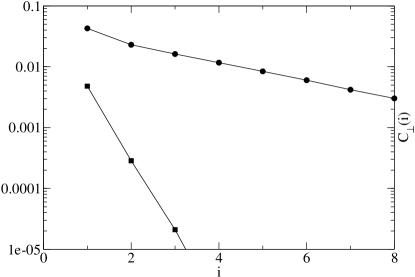
Figure 13: Transverse spin-spin correlation as function of the distance for $J_{\perp}=0.4$, $J_{d}=0$ (circles), $J_{\perp}=0.4$, $J_{d}=0.219$ (squares).

III.5 Finite size spin gap

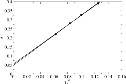
Figure 14: Finite size gap with OBC as function of the lattice size for $J_{\perp}=0$ (circles) and, $J_{\perp}=0.2$ (squares).

Logarithmic corrections and the spurious dimerization introduced by the OBC is accompanied by a spurious gap in the pure 1D system. In Fig.( 14) we see that at the maximally frustrated point, the gap for $J_{\perp}=0.2$ converges to the same value as that of $J_{\perp}=0$. It is thus reasonable, knowing that the single chain is gapless, to conclude that the 2D system is also gapless in the thermodynamic limit. We note that the logarithmic corrections are not taken into account in the gaps predicted by exact diagonalization studiessindzingre .

III.6 Implications for the isotropic $J_{1}-J_{2}$ model

For the isotropic case ($J_{\perp}=J$) it is usually said that there is a large amount of evidence supporting the fact that the magnetic order vanishes for $0.4\lesssim J_{d}\lesssim 0.6$, i.e., a spin gapped state exists in this region lhuillier . But in our opinion, this conclusion is not that compelling. The results displayed above indicate that the limit $J_{d}/J_{\perp}\rightarrow 0.5$ is in fact analogous to the problem of coupled unfrustrated chains ($J_{d}=0$ in Hamiltonian( 1)) in the limit $J_{\perp}\rightarrow 0$. For this latter problem there was a prediction of a spin liquid state for $J_{\perp}\lesssim 0.1$ from ED, field theory mapping and spin wave approaches parola . However, a QMC study sandvik later showed that the Néel order extends down to $J_{\perp}=0.01$. It is now believed that long-range order sets in as soon as $J_{\perp}\neq 0$. This suggests that the disordered phase often claimed to exists for the isotropic $J_{1}-J_{2}$ model, which was obtained from ED of only a maximum of $6\times 6$ systems or series expansions such as dimers expansions which may be biased toward dimerization, is not a settled issue.

In fact there is a strong evidence, unfortunately neglected, which points to the contrary. A DMRG study wang performed on a three-leg ladder found that the system is gapless for all values of $J_{\perp}$ and $J_{d}$. The lenght of the chains were up to $L=360$ so that finite size effects were negligible. The computed phase diagram has two states a symmetric doublet phase and the quartet phase. The low energy properties of the symmetric doublet phase are similar to those of a single spin-$1/2$ chain. The scaling behavior of the quartet phase is identical to that of a spin-$3/2$. These two states will naturally evolve towards the Néel $Q=(\pi,\pi)$ and $Q=(\pi,0)$, respectively, when the number of chains goes to infinity. This is fully consistent with our conclusions.

The perturbative method applied in this study cannot be used directly to study the isotropic case, since starting with the decoupled chains is too biased. But if the principles uncovered in the anisotropic case are to be applied, it appears that even in the isotropic situation, the nearly decoupled chains ground state is still the best way to minimize frustration. From this consideration, we applied the method to the isotropic case and arrived at the same conclusions as above. Namely that the ground state at the maximally frustrated point is made of nearly disconnected chains and is thus a SLL.

Another indication for this is the finding by a recent ED study sindzingre that even at $J_{\perp}=0.8J$ the behavior observed at lower coupling still persists. However, this study also predicts a spin gap. We believe this apparent contradiction is due to the fact that the ED study was done with an even number of chains and the logarithmic corrections were not considered.

IV Doped systems

Having identified the ground state at half-filling as a spin version of a SLL, we now turn to the doped case. We will mostly restrict ourselves to the vicinity of the maximally frustrated point $J_{d}\approx J_{\perp}/2$. This is primarily because the results at half-filling indicate that far from this point no significantly new physics is likely to occur. One would expect that the two Néel ground states found at half-filling away from the the QCP will naturally evolve into spin density wave (SDW) ground states upon doping. The really physically interesting question is: What is the effect of the doping upon the spin SLL?

The main finding in the doped case is that the magnetic properties of the system do not significantly change as long as one remains close to half-filling. But if the hole doping becomes too large, $x\approx 0.3$, the model displays a qualitative change. The frustration ceases, and $J_{d}$ cooperates instead of competing with $J_{\perp}$.

IV.1 Ground-state energies

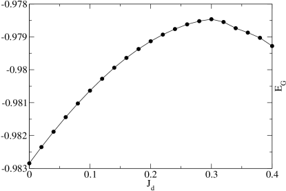
Figure 15: Ground state energy for $x=0.167$, $L=12$, and $J_{\perp}=0.4$ as function of $J_{d}$.

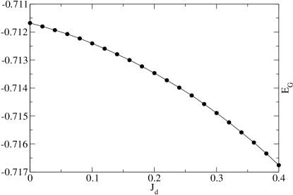
Figure 16: Ground-state energy for $x=0.4$, $L=10$, and $J_{\perp}=0.2$ as function of $J_{d}$

$E_{G}$ at $x=0.167$ for $L=12$ as function of $J_{d}$ is shown in Fig.( 15). It displays a maximum as for the half-filled case. One can note that this maximum is now shifted towards higher values of $J_{d}$. This maximum goes from $J_{d}^{max}=0.236$ for $x=0$ to $J_{d}^{max}=0.30$ for $x=0.167$. By inserting the holes, the system becomes less frustrated. It is therefore necessary to increase $J_{d}$ in order to balance the action of $J_{\perp}$. We find that if the hole density is increased above $x\approx 0.3$ the maximum in $E_{G}$ is suppressed. For $x\gtrsim 0.3$, $E_{G}$ always decreases with $J_{d}$. This is seen for instance in Fig.( 16) where $E_{G}$ for $x=0.4$ is shown. This shows that for large dopings, contrary to the near half-filling situation, $J_{d}$ increases instead of reducing the stability of the system.

IV.2 Short-distance spin-spin correlations

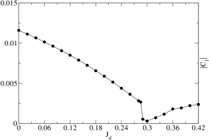
Figure 17: $C_{1}$ for $x=0.167$, $L=12$, and $J_{\perp}=0.4$ as function of $J_{d}$

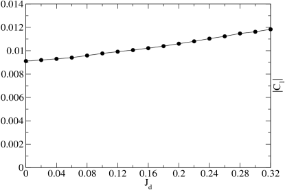
Figure 18: $C_{1}$ for $x=0.4$, $L=10$, and $J_{\perp}=0.2$ as function of $J_{d}$

This difference between the near half-filling and larger hole densities is also displayed in $C_{1}$. In Fig.( 17) corresponding to $x=0.167$, $C_{1}$ goes to $0$ at $J_{d}^{0}=0.3$. One may note that there seems to be a jump at the transition point. This jump was not observed at half-filling. This could indicate a possible first order transition. However this is not supported by the behavior of $E_{G}$ shown above. We notice during the simulations that, if one is too close to the transition point, for the same set of parameters, one can go from one side of the transition when the number of chains is small to the other side when the number of chains gets larger. We thus believe that the jump observed in $C_{1}$ is somehow related to the reduced accuracy in the doped case induced by the mixture of the two competing ground states near the transition point. The regularity of the curve far from the transition point justify this assumption. In agreement with the behavior of $E_{G}$, the transition is suppressed when the hole doping is too large. $C_{1}$ shown in Fig.( 18) always remain antiferromagnetic and increases with $J_{d}$.

IV.3 Long-distance correlations

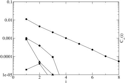
Figure 19: Transverse spin-spin correlation as function of the distance for $J_{\perp}=0.2$, $J_{d}=0$ (circles), and at the maximally frustrated point at $J_{\perp}=0.2$ (squares), $J_{\perp}=0.4$ (triangles), $J_{\perp}=0.6$ (diamonds).

$C_{\perp}(i)$ shown in Fig.( 19) for $x=0.125$ retains essentially the same behavior as in the half-filled case. It decays exponentially at the maximally frustrated point for $J_{\perp}=0.2$, $0.4$, and $0.6$ while the decay is significantly slower in the unfrustrated case. In the absence of frustration, $C_{\perp}(i)$ has an antiferromagnetic signature while $C_{\parallel}(i)$ is SDW like with $k_{F}=\frac{\pi}{2}(1-x)$, where $x$ is the density of holes. Though we have not made a finite size analysis, it is reasonable to believe that the system is in an SDW ground state in the thermodynamic limit. At the maximally frustrated point, the magnetic order parameter vanishes.

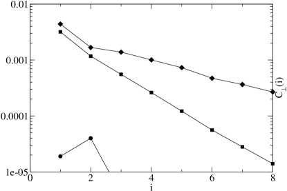
Figure 20: Transverse spin-spin correlation as function of the distance for $J_{\perp}=0.2$,$J_{d}=0.11$ for $x=0.125$ (circles), $x=0.25$ (squares) and $x=0.375$ for $L=16$.

As $x$ is further increased to $0.167$, $0.25$, and $0.375$, we find that the role of frustration is reduced. Ultimately, the system evolves towards a conventional SDW ground state. This is seen in Fig.( 20) where the exponential decay of $C_{\perp}(i)$ is significantly slowed at large hole dopings. There is already four orders of magnitudes between $C_{\perp}(4)$ for $x=0.125$ and $x=0.375$. It appears that the system tends to choose hole configurations that minimize frustration in order to avoid the cost in energy induced by frustration. It is in the vicinity of $x=0.125$ that frustration is most effective, i.e., the magnetic order which exists in the non-frustrated case can easily be cancelled by frustration. Beyond this point, frustration becomes less and less effective. At quarter filling the system can choose a hole configuration so that frustration becomes ineffective. Such possible configurations are shown in Fig. (24), but we have not made a systematic analysis of them. Since the introduction of holes usually tends to reduce the order parameter, the reemergence of magnetism at the maximally frustrated point by introduction of holes can be viewed as the manifestation of Villain’s order from disorder effect villain .

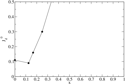
Figure 21: Critical values of $J_{d}$ as function of doping.

These arguments are illustrated in Fig.( 21) where the value of $J_{d}^{0}$ is shown as function of $x$. $J_{d}^{0}(x)$ first slowly decreases from half-filling until about $x=0.125$ and then sharply rises. Thus there is a point, for $x$ between $0.25$ and $0.5$, where the critical point is suppressed.

IV.4 Equal-time Green’s function

The transition point is also signaled in the equal-time transverse Green’s function

$$G_{\perp}(i)=\langle c_{jl\sigma}c^{\dagger}_{jl+i\sigma}\rangle.$$ (15)

$G_{1}=G_{\perp}(1)$ is shown in Fig.( 22) decays from $J_{d}=0$ to $J_{d}=J_{d}^{max}$. This decay of $G_{1}$ is consistent with the tendency to localize the particles within the chains induced by $J_{d}$. However, in the vicinity of $J_{d}^{max}$, the situation becomes less clear. $G_{1}$ strongly oscillates. These oscillations cease when $J_{d}$ is beyond the critical region where $G_{1}$ decays again. It appears that $G_{1}$ behaves differently in the two ordered states; it increases from the transition point in the first and decreases from the transition point in the second state. The curious behavior seen in the transition region could well be the manifestation of the mixture of the two ground states seen in $E_{G}$ and in $C_{1}$. This mixture affects the value of fermion correlation functions more severely than their spin counterpart. For this reason, we have not calculated charge density or superconducting correlations which involve four fermions. There is however no reason to suspect a charge density or superconducting ordering in the vicinity of $J_{d}^{max}$. These transition would be of first order and would thus be apparent in the ground state energy.

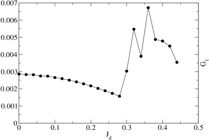
Figure 22: Transverse equal-time first neighbors Green’s function at $x=0.167$ as function of $J_{d}$ for $L=12$.

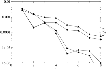
Figure 23: Transverse equal-time Green’s function at $x=0.125$ for $J_{d}=0.2$, $J_{d}=0$ for spin up (circles), spins down (squares); $J_{\perp}=0.2$,$J_{d}=0.11$ for spins up (triangles), spins up (diamonds)

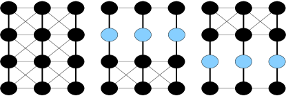
Figure 24: Holes (light color) configurations that minimize frustration for $x=0.25$. The left illustration represents the half-filled case where the system is fully frustrated.

Despite the uncertainties caused by the mixture of the two ground states on the two sides of the transition, we nevertheless show in Fig.( 23) the equal-time transverse Green’s function in the SDW case and in the magnetically disordered case. The decay in the disordered state is slower than in the magnetic case. This raises the possibility of the relevance of the single particle hopping. If true, this would mean that the spin and the charge behave differently in the transverse direction at the transition point. More work needs to be done in order to clarify this point.

V Conclusions

In this study, we have presented numerical evidence for the connection between quantum phase transition and Luttinger liquid physics from the study of coupled $t-J$ chains. The ordered $Q=((1-x)\pi,\pi)$ Néel state that exists at half-filling and near half-filling for $J_{\perp}\neq 0$ and $J_{d}=0$ is destroyed at $J_{d}=J_{d}^{max}$. At this point, the in-chain spin-spin correlation of the 2D system decay nearly like those of independent chains. A careful examination of the transverse spin-spin correlations reveals that the chains are loosely bound and that these correlations decay exponentially. We thus identify the state of the system at this maximally frustrated point as a sliding Luttinger liquid. These properties are observed even when the interchain coupling are well beyond the perturbative regime

The key mechanism behind this connection is magnetic frustration. The leading effect which brings a compromise between the frustrated bonds is the severing of these bonds to form the largest unfrustrated clusters with the lowest energy. These unfrustrated units are then coupled by some residual interactions generated by quantum fluctuations. These residual interactions may or may not drive the system away from the physics displayed by the largest unfrustrated clusters. This picture is in constrast to the widely accepted hypothesis which suggests that the leading mechanism to avoid frustration is short or long-range dimerization which may (spin-Peierls) or may not (Resonating Valence Bond) lead to the breaking of the lattice translational symmetry. It is however to be noted that the two pictures do not necessarily always conflict with each other. In some models, the largest unfrustrated clusters could just be dimers or plaquettes. Our point here is that this is not the case in the anisotropic $J_{1}-J_{2}$ model.

In the model studied in this paper, LL physics arises at the QCP because the severing of frustrated bonds leads to nearly independent chains which are the largest unfrustrated clusters. These chains are coupled, even when the original interchain couplings are large, only by residual interactions which do not appear to destabilize the 1D physics at the QCP. In a numerical simulation, it is however impossible to rule out completely the emergence of relevant interchain interactions at a very low energies.

- (1) J.Orenstein and A.J. Millis, Science 288, 468 (2000).
- (2) C. Bourbonnais and D. Jérome in ”Advance in Synthetic Metals” Eds. P. Bernier, S. Lefrant and G. Bidan (Elsevier, New York), 206 (1999).
- (3) J.W. Allen, Sol. St. Comm. 123, 469 (2002).
- (4) P.W. Anderson, Science 288, 480 (2000).
- (5) S. Kivelson, Synthetic Metals 125, 99 (2002).
- (6) S. Sachdev ”Quantum Phase Transitions”, Cambridge University Press (1999).
- (7) C. Bourbonnais and L.G. Caron, Int. J. Mod. Phys. B 5, 1033 (1991).
- (8) R. Shankar, Rev. Mod. Phys. 66, 129 (1994).
- (9) A. Vishwanath and D. Carpentier, Phys. Rev. Lett. 86, 676 (2001).
- (10) V.J Emery, E. Fradkin, S.A. Kivelson, and T.C. Lubensky, Phys. Rev. Lett. 85, 2160 (2000).
- (11) R. Mukhopadhyay, C.L. Kane, and T.C. Lubensky, Phys. Rev. B 64, 045120 (2001).
- (12) R.B. Laughlin, Adv. Phys. 47, 943 (1998).
- (13) S. Moukouri and L.G. Caron, Phys. Rev. B 67, 092405 (2003).
- (14) S. Moukouri, Phys. Rev. B 70, 014403 (2004) .
- (15) S. Moukouri. Phys. Lett. A 325 177.
- (16) A. A. Nersesyan and A. M. Tsvelik Phys. Rev. B 67, 024422 (2003); A. M. Tsvelik Phys. Rev. B 70, 134412 (2004).
- (17) O. A. Starykh and L. Balents Phys. Rev. Lett. 93, 127202 (2004).
- (18) J.V. Alvarez and S. Moukouri cond-mat/0402530 (unpublished).
- (19) S. Moukouri and J.V. Alvarez cond-mat/0403372.
- (20) T. Kato, Prog. Teor. Phys. 4, 514 (1949); 5, 95 (1950).
- (21) C. Bloch, Nucl. Phys. 6, 329 (1958).
- (22) S.R. White, Phys. Rev. Lett. 69, 2863 (1992). Phys. Rev. B 48, 10 345 (1993).
- (23) G. Misguich and C. Lhuillier in ”Frustrated Spin Systems” Ed. H.T. Diep World Scientific (2004).
- (24) A. Sindzingre, Phys. Rev. B 69, 094418 (2004).
- (25) A. Parola, S. Sorella and Q.F. Zhong, Phys. Rev. Lett. 71, 4393 (1993).
- (26) A. Sandvik, Phys. Rev. Lett. 83, 3069 (1999).
- (27) X. Wang, N. Zhu, C. Chen, Phys. Rev. B 66 172405 (2002).
- (28) I. Affleck and S. Qin, J. Phys. A 32, 7815 (1999).
- (29) J. Villain, R. Bidaux, J.-P. Carton, and R. Conte, J. Phys (France) 41, 1263 (1980).