Variational matrix product state approach to quantum impurity models

Abstract

We present a unified framework for renormalization group methods, including Wilson’s numerical renormalization group (NRG) and White’s density-matrix renormalization group (DMRG), within the language of matrix product states. This allows improvements over Wilson’s NRG for quantum impurity models, as we illustrate for the one-channel Kondo model. Moreover, we use a variational method for evaluating Green’s functions. The proposed method is more flexible in its description of spectral properties at finite frequencies, opening the way to time-dependent, out-of-equilibrium impurity problems. It also substantially improves computational efficiency for one-channel impurity problems, suggesting potentially linear scaling of complexity for $n$-channel problems.

Wilson’s numerical renormalization group (NRG) is a key method Wilson for solving quantum impurity models such as the Kondo, Anderson or spin-boson models, in which a local degree of freedom, the “impurity”, is coupled to a continuous bath of excitations. These models are of high relevance in the description of magnetic impurities, of quantum dots, and problems of decoherence. NRG has been used with great success to calculate both thermodynamic Wilson ; Krishna and dynamical Costi ; Hofstetter ; Raas properties. It is, however, of limited use in more complex situations: Computational cost grows exponentially for a coupling to multiple bands in the bath. In systems out of equilibrium or with time-dependent external parameters, such as occur in the tuning of quantum dots, difficulties arise due to NRG’s focus on low energy properties through its logarithmic discretization scheme which looses accuracy at high spectral frequencies.

In the present Letter, we draw attention to the fact that states generated by the NRG have the structure of matrix product states (MPS) AKLT+Fannes ; VPC on a 1-D geometry. This is a simple observation, which however has important conceptual and practical implications:

(i) As White’s density matrix renormalization group (DMRG) White for treating quantum chain models is in its single-site version identical to variational MPS VPC , NRG and DMRG are now seen to have the same formal basis of matrix product states, resolving a long-standing question about the connection between both methods. (ii) All NRG results can be improved upon systematically by variational optimization in the space of variational matrix product states (VMPS) of the same structure as those used by NRG. This does not lead to major improvements at $\omega=0$ where NRG works very well, but leads to the inclusion of feedback from low- to high-energy states, also allowing the relaxation of the logarithmic bath discretization of NRG: spectra away from $\omega=0$ can be described more accurately and with higher resolution. (iii) Recent algorithmic advances using VMPS VPC , in particular those treating time-dependent problems t-methods ; VGC , can now be exploited to tackle quantum impurity models involving time-dependence or nonequilibrium; this includes applications to the description of driven qubits coupled to decohering baths, as relevant in the field of quantum computation. (iv) The VMPS algorithm allows ground state properties of quantum impurity models to be treated more efficiently than NRG: the same accuracy is reached in much smaller ansatz spaces (roughly, of square-root size). Moreover, our results suggest that for many (if not all) $n$-channel impurity problems it should be feasible to use an unfolded geometry, for which the complexity will only grow linearly with $n$.

The present Letter provides a “proof of principle” for the VMPS approach to quantum impurity models by applying it to the one-channel Kondo model. We reproduce the NRG flow of the finite size spectrum Krishna , and introduce a VMPS approach for calculating Green’s functions, as we illustrate for the impurity spectral function Costi , which yields a significant improvement over existing alternative techniques GreensDMRG1 ; GreensDMRG2 ; GreensDMRG3 ; othermethods . Our results illustrate in which sense the VMPS approach is numerically more efficient than the NRG.

NRG generates matrix product states:— To be specific, we consider Wilson’s treatment of the Kondo model, describing a local spin coupled to a fermionic bath. To achieve a separation of energy scales, the bath excitations are represented by a set of logarithmically spaced, discrete energies $\omega_{n}=\Lambda^{-n}$, where $\Lambda>1$ is a “discretization parameter” Wilson . By tridiagonalization, the model is then mapped onto the form of a semi-infinite chain $\mathcal{H}=\lim_{N\to\infty}\mathcal{H}^{N}$ where Wilson

$$\mathcal{H}^{N}=-2J\mathbf{s}\cdot\mathbf{S}+\sum_{n=1}^{N-1}\xi_{n}\left(c_{n\mu}^{\dagger}c_{n+1,\mu}+c_{n+1,\mu}^{\dagger}c_{n\mu}\right)$$ (1)

with $\mathbf{S}\equiv\textstyle{\frac{1}{2}}c_{0}^{\dagger}\mathbf{\boldsymbol{\sigma}}c_{0}$ and creation (annihilation) operators $c^{\dagger}\,(c)$, respectively. $\mathcal{H}^{N}$ describes an impurity spin $\mathbf{s}$ coupled to the first site of a chain of length $N$ of Fermions with spin $\mu$ and exponentially decreasing hopping matrix elements along the chain ($\xi_{n}\sim\Lambda^{-n/2}$). $\mathcal{H}^{N}$ lives on a Hilbert space spanned by the set of $d_{I}d^{N}$ basis states $\{|i_{0},i_{1},i_{2},\dots i_{N}\rangle\}$, where $i_{0}$ labels the $d_{I}$ possible impurity states and $i_{n}$ (for $n=1,\dots,N$) the $d$ possible states of site $n$ (for the Kondo model, $i_{0}=\left\{\uparrow,\downarrow\right\}$ and for all other sites $i_{n}=\left\{0,\uparrow,\downarrow,\uparrow\downarrow\right\}$, i. e. $d_{I}=2$ and $d=4$).

To diagonalize the model, NRG starts with a chain of length $(\bar{n}-1)$, chosen sufficiently small that $\mathcal{H}^{\bar{n}-1}$ can be diagonalized exactly, yielding a set of eigenstates $|\psi_{\alpha}^{\bar{n}-1}\rangle$. One continues with the subsequent iterative prescription: project $\mathcal{H}^{\bar{n}-1}$ onto the subspace spanned by its lowest $D$ eigenstates, where $D<d_{I}d^{\bar{n}-1}$ is a control parameter (typically between 500 and 2000); add site $\bar{n}$ to the chain and diagonalize $\mathcal{H}^{\bar{n}}$ in the enlarged $(Dd)$-dimensional Hilbert space, writing the eigenstates as

$$|\psi^{\bar{n}}_{\beta}\rangle=\sum_{i_{\bar{n}}=1}^{d}\sum_{\alpha=1}^{D}|\psi^{\bar{n}-1}_{\alpha}\rangle|i_{\bar{n}}\rangle\,P^{[i_{\bar{n}}]}_{\alpha\beta}\;,$$ (2)

where the coefficients have been arranged in a matrix $P^{[i_{\bar{n}}]}_{\alpha\beta}$ with matrix indices $\alpha,\beta$, labelled by the site index $\bar{n}$ and state index $i_{\bar{n}}$; rescale the eigenenergies by a factor $\Lambda^{1/2}$; and repeat, until the eigenspectrum converges, typically for chain lengths $N$ of order 40 to 60. At each step of the iteration, the eigenstates of $\mathcal{H}^{N}$ can thus be written [by repeated use of Eq. (2)] in the form of a so-called matrix product state,

$$|\psi^{N}_{\alpha}\rangle = P^{[i_{0}]}_{\alpha_{0}}P^{[i_{1}]}_{\alpha_{0}\alpha_{1}}P^{[i_{2}]}_{\alpha_{1}\alpha_{2}}\ldots P^{[i_{N}]}_{\alpha_{N-1}\alpha}|i_{0},i_{1},\dots,i_{N}\rangle\qquad\phantom{.}$$ (3)

(summation over repeated indices implied). The ground state is then the lowest eigenstate of the effective Hamiltonian $\mathcal{H}^{N}_{\alpha\beta}=\langle\psi^{N}_{\alpha}|\mathcal{H}^{N}|\psi^{N}_{\beta}\rangle$, i.e. the projection of the original $\mathcal{H}$ on the subspace of MPS of the form (3).

VMPS optimization:— Let us now be more ambitious, and aim to find the best possible description of the ground state within the space of all MPSs of the form (3), using the matrix elements of the matrices $\{P^{[n]}\}$ with $P^{[n]}\equiv\{P^{[i_{n}]}\}$ as variational parameters to minimize the energy. Using a Lagrange multiplier to ensure normalization, we thus study the following optimization problem:

$$\min_{|\psi^{N}\rangle\in\{{\rm MPS}\}}\left[\langle\psi^{N}|\mathcal{H}^{N}|\psi^{N}\rangle-\lambda\langle\psi^{N}|\psi^{N}\rangle\right].$$ (4)

This cost function is multiquadratic in the $d_{I}+d(N-1)$ matrices $\{P^{[n]}\}$ with a multiquadratic constraint. Such problems can be solved efficiently using an iterative method in which one fixes all but one (let’s say the $\bar{n}$’th) of the matrices $\{P^{[n]}\}$ at each step; the optimal $P^{[\bar{n}]}$ minimizing the cost function given the fixed values of the other matrices can then be found by solving an eigenvalue problem VPC . With $P^{[n]}$ optimized, one proceeds the same way with $P^{[\bar{n}+1]}$ and so on. When all matrices have been optimized locally, one sweeps back again, and so forth. By construction, the method is guaranteed to converge as the energy goes down at every step of the iteration, having the ground state energy as a global lower bound. Given the rather monotonic hopping amplitudes, we did not encounter problems with local minima.

In contrast, NRG constructs the ground state in a single one-way sweep along the chain: each $P^{[n]}$ is thus calculated only once, without allowing for possible feedback of $P$’s calculated later. Yet viewed in the above context, the ground state energy can be lowered further by MPS optimization sweeps. This accounts for the feedback of information from low to high energy scales. This feedback may be small in practice, but it is not strictly zero, and its importance increases as the logarithmic discretization is refined by taking $\Lambda\to 1$. Note that the computational complexity of both VMPS optimization and NRG scales as $NdD^{3}$ White ; VPC , and symmetries can be exploited (with similar effort) in both approaches. The inclusion of feedback leads to a better description of spectral features at high frequencies, which are of importance in out-of-equilibrium and time-dependent impurity problems. Moreover, it also allows to relax the logarithmic discretization scheme, further improving the description of structures at high frequency as illustrated below.

Energy level flow:— The result of a converged set of optimization sweeps is a VMPS ground state $|\tilde{\psi}_{0}^{N}\rangle$ of the form (3); exploiting a gauge degree of freedom VPC , the $\tilde{P}$’s occurring therein can always be chosen such that all vectors $|\tilde{\psi}_{\alpha}^{n}\rangle=\bigl{[}\tilde{P}^{[i_{0}]}\dots\tilde{P}^{[i_{n}]}\bigr{]}_{\alpha}|i_{0},\dots,i_{n}\rangle$ are orthonormal. The effective Hamiltonian at chain length $n$, the central object in NRG, is then $\tilde{\mathcal{H}}^{n}_{\alpha\beta}=\langle\tilde{\psi}^{n}_{\alpha}|\Lambda^{n/2}\mathcal{H}^{n}|\tilde{\psi}^{n}_{\beta}\rangle$. Its eigenspectrum can be monitored as $n$ increases, resulting in an energy level flow along the chain.

Green’s functions:— Similar techniques also allow Green’s functions to be calculated variationally othermethods . The typical Green’s functions of interest are of the form $G_{\eta}^{c}(\omega)=\langle\psi_{0}|c|\chi\rangle$ where $|\chi\rangle$, commonly called a correction vector Soos , is defined by

$$|\chi\rangle\equiv\frac{1}{\omega-\mathcal{H}+i\eta}c^{\dagger}|\psi_{0}\rangle\;,$$ (5)

with $|\psi_{0}\rangle$ the ground state of the system, e. g. calculated using the VMPS approach and thus represented as MPS. The spectral density is then given by ${\cal A}(\omega)=-\lim_{\eta\rightarrow 0}\frac{1}{\pi}\Im\mathrm{m}\left(G_{\eta}^{c}(\omega)\right)$. The (unnormalized) state $|\chi\rangle$ may be calculated variationally within the set of MPS by optimizing the weighted norm

$$\mathcal{N}=\left\|\chi\rangle-\frac{1}{\mathcal{H}-\omega-i\eta}c^{\dagger}|\psi_{0}\rangle\right\|_{W=\left(\mathcal{H}-\omega\right)^{2}+\eta^{2}},$$ (6)

where $\|\xi\rangle\|_{W}^{2}\equiv\langle\xi|W|\xi\rangle$, and weight $W>0$ such that it yields a quadratic equation. Minimizing $\mathcal{N}$ efficiently by optimizing one $P$ at a time leads to two independent optimizations over $\Re\mathrm{e}|\chi\rangle$ and $\Im\mathrm{m}|\chi\rangle$, respectively. Both involve only multilinear terms such that each iteration step requires to solve a sparse linear set of equations VGC .

The minimization of ${\cal N}$ in Eq. (6), however, can become increasingly ill-conditioned as $\eta\rightarrow 0$ EPAPS , with conditioning deteriorating quadratically in $\eta$. If one directly solves $\delta/\delta\langle P^{[n]}|\ \left[\langle\chi|(\mathcal{H}-\omega-i\eta)|\chi\rangle-\langle\chi|c^{\dagger}|\psi\rangle\right]\equiv 0$ by a non-hermitian equation solver such as the biconjugate gradient method, conditioning deteriorates only linearly.

Application to Kondo model:— Let us now illustrate above strategies by applying them to the Kondo model. Since the Hamiltonian in Eq. (1) couples $\uparrow$ and $\downarrow$ band electrons only via the impurity spin, it is possible (see also Raas ; Saberi08 ) to “unfold” the semi-infinite Wilson chain into an infinite one, with $\uparrow$ band states to the left of the impurity and $\downarrow$ states to the right, and hopping amplitudes decreasing in both directions as $\Lambda^{-|n|/2}$. Since the left and right end regions of the chain, which describe the model’s low-energy properties, are far apart and hence interact only weakly with each other (analyzed quantitatively in terms of mutual information in Fig. 1b), the effective Hamiltonian for these low energies will be of the form ${\cal H}^{\rm eff}_{\uparrow}\otimes 11_{\downarrow}+11_{\uparrow}\otimes{\cal H}^{\rm eff}_{\downarrow}$. Due to the symmetry of the Kondo coupling, ${\cal H}^{\rm eff}_{\uparrow}$ and ${\cal H}^{\rm eff}_{\downarrow}$ have the same eigenspectrum for $n\gg 1$, such that the fixed point spectrum is already well-reflected by analyzing either one, as illustrated in Fig. 1(a). Note that for a direct comparison with NRG, the spin chains can be recombined within VMPS Saberi08 . The resulting standard energy flow diagram presented in panel (a) for VMPS and NRG, respectively, show excellent agreement for low energies for all $n$ including the fixed point spectrum.

The dimensions of the effective Hilbert spaces needed for VMPS and NRG to capture the low energy properties (here energy resolution better than $T_{K}$) are roughly related by $D_{\rm MPS}\sim\sqrt{D_{\rm NRG}}$ Saberi08 ), implying significant computational gain with VMPS, as calculation time scales as $D^{3}$ for both. Indeed, Fig. 1(e) shows that VMPS has three orders of magnitude of better precision for the same $D$. More generally, if the impurity couples to $n$ electronic bands (channels), the Wilson chain may be unfolded into a star-like structure of $2n$ branches, with $D_{\rm MPS}\sim D_{\rm NRG}^{1/2n}$. This implies that for maintaining a desired precision in going from 1 to $n$ channels, $D_{\rm MPS}$ will stay roughly constant, and calculation time for all sites other than the impurity will scale merely linearly with the number of channels. Whether the chains can be unfolded in practice can easily be established by checking whether or not the correlation between them, characterized e.g. in terms of mutual information, decays rapidly with increasing $n$ (cf. Fig. 1b and caption).

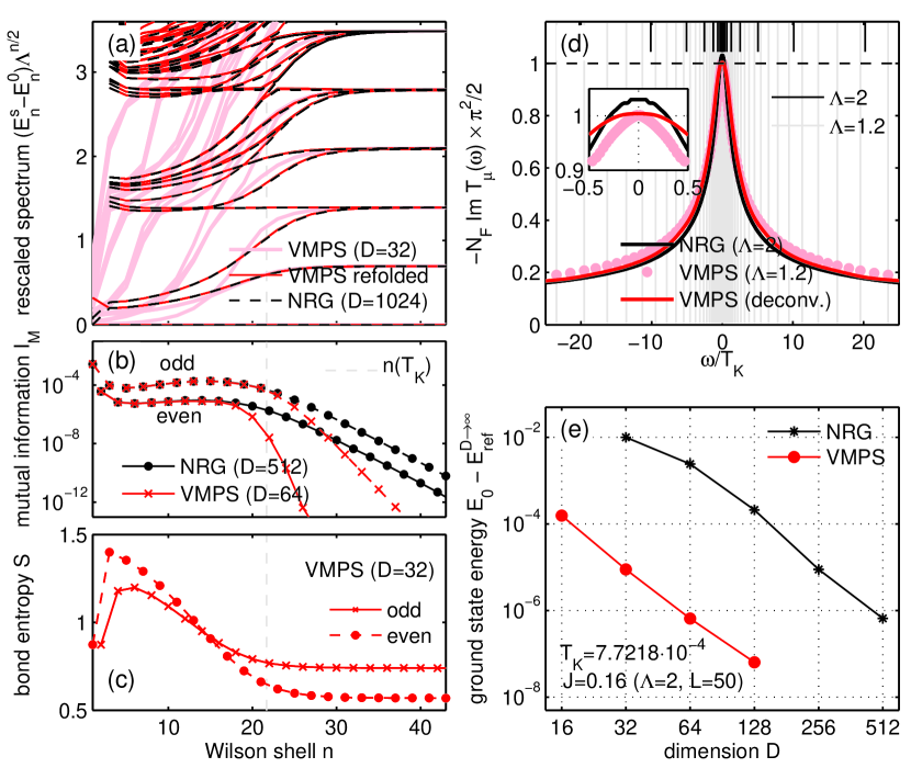
Figure 1: (Color online) Comparison of VMPS and NRG data for logarithmic discretization. (a) Energy level flow of the Kondo model as a function of site index $n$ obtained from ${\cal H}^{\rm eff}_{\mu}$ of a variationally optimized MPS with $D_{{\rm MPS}}=32$ (light red), of the corresponding recombined spin chains (red) Saberi08 , and from NRG using $D_{{\rm NRG}}=32^{2}$ states (dashed black). (b) Correlation along the Wilson chain between spin-up and spin-down at site $n$ in terms of mutual information $I_{M}(n)\equiv S({n_{\uparrow}})+S({n_{\downarrow}})-S(n_{\uparrow},n_{\downarrow})$. Here $S$ is the entropy of the reduced density matrix of the groundstate with respect to the indicated subspace Saberi08 (solid for even, dashed for odd sites $n$). The Wilson shell corresponding to $T_{K}$ is indicated by the vertical dashed line. (c) Bond entropy $S$ along the unfolded Wilson chain where $S$ is the usual von Neumann entropy of the VMPS reduced density matrix when going from site $n$ to $n+1$. (d) Comparison of $T$-matrix ($\Im\mathrm{m}\,T_{\mu}$, see also Fig. 2) for $B=0$ between VMPS and NRG, including deconvoluted VMPS data EPAPS . Inset shows zoom into peak at $\omega=0$. The significantly smaller $\Lambda=1.2$ applicable for VMPS (discretization intervalls are indicated by vertical lines) shows clearly improved agreement with the Friedel sum rule $T\left(0\right)\,\pi^{2}/2=1$. (e) Comparison of ground state energy of the Kondo Hamiltonian (1) for fixed chain length relative to the extrapolated energy for $D\rightarrow\infty$ for VMPS and NRG as function of the dimension $D$ of states kept.

Adaptive discretization:— Through its variational character, VMPS does not rely on logarithmic discretization crucial for NRG. The potential of greatly enhanced energy resolution using VMPS is already indicated by the $\Lambda=1.2$ data in Fig. 1(d). It is illustrated to full extent in Fig. 2, showing the splitting of the Kondo peak in the presence of a strong magnetic field calculated using VMPS (bare: dots, deconvoluted: red solid), standard NRG (blue dashed) and perturbatively Rosch03 (black). By using a linear (logarithmic) discretization scheme for $|\omega|\!<\!B$ ($|\omega|\!>\!B$), respectively, VMPS yields well-resolved sharp spectral features at finite frequencies. This resolution is out of reach for NRG, whose discretization intervals (blue shaded intervals), even for comparatively small choice of $\Lambda=1.7$, are much broader than the spectral features of interest. The line shape of our deconvoluted data (red solid line) agrees well with the analytic RG calculation Rosch03 (black solid line), perturbative in $1/\log(B/T_{K})$. The peak positions agree well also after a shift in $\omega$ by $-B/2\log(B/T_{K})$ of the perturbative result suggested by Rosch03 is taken into account.

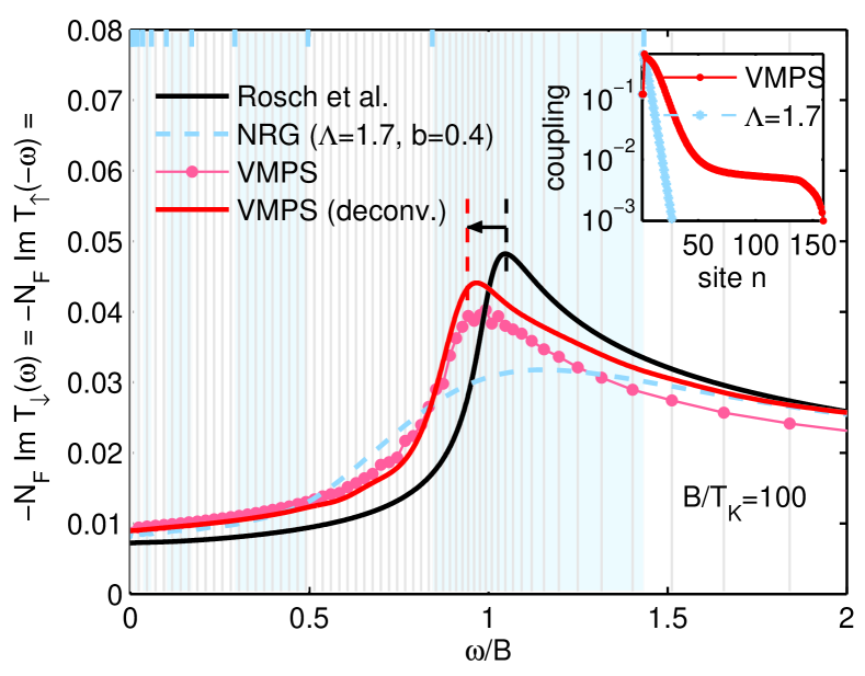
Figure 2: (Color online) Impurity spectral function for the Kondo model $-N_{F}\,\Im\mathrm{m}\,T_{\mu}(\omega)=J^{2}\langle\langle\mathcal{O}_{\mu}^{\dagger}|\mathcal{O}_{\mu}\rangle\rangle_{\omega}$ for $B\gg T_{K}$, where $\mathcal{O}_{\mu}\equiv\mathbf{S}\cdot\mathbf{\sigma}_{\mu\mu^{\prime}}c_{\mu^{\prime}}^{\dagger}$ and $N_{F}$ is the density of states at the Fermi energy, calculated with VMPS (dots: raw data, red solid: deconvoluted), NRG (dashed) and perturbative (black solid) Rosch03 . According to Rosch03 , the peak of the perturbative result should be shifted in $\omega$ by $-B/2\log(B/T_{K})$ (arrow). NRG and VMPS discretization intervals are indicatd by blue shaded areas and gray vertical lines, respectively. The inset shows the hopping amplitudes corresponding to standard (blue dashed) and adapted (red solid) discretization schemes. The required Lorentzian broadening $\eta$ of the VMPS data smears out sharper features. Deconvolution (targeting with adaptive spline) together with subsequent Gaussian broadening was applied to obtain the red solid line EPAPS .

Outlook:— Let us finish by pointing out that the MPS approach can readily be extended to the case of finite temperatures by using matrix product density operators VGC instead of MPS, and to time-dependent problems (such as $\mathcal{H}=\mathcal{H}(t)$ or non-equilibrium initial conditions), by using the recently developed adaptive time-dependent DMRG t-methods and MPS analogues thereof VGC . Preliminary work in this direction was very encouraging and will be published in the near future.

In conclusion, the MPS approach provides a natural language for simulating quantum impurity models. The underlying reason is that these models, when formulated on the Wilson chain, feature only nearest-neighbor interactions. Their low-energy states are thus determined mainly by their nearest-neighbor reduced density matrices, for which very good approximations can be obtained by suitably optimizing the set of matrices constituing a MPS VC05 . We also showed how these could be used for a direct variational evaluation of Green’s functions.

We gratefully acknowledge fruitful discussions with M. Sindel, W. Hofstetter, G. Uhrig and F. Anders. This work was supported by DFG (SFB 631, SFB-TR 12, De 730/3-1, De 730/3-2), GIF (I-857), European projects (Spintronics RTN, SCALA), Kompetenznetzwerk der Bayerischen Staatsregierung Quanteninformation, and the Gordon and Betty Moore Foundation (Information Science and Technology Initiative, Caltech). Financial support of the Excellence Cluster Nanosystems Initiative Munich (NIM) is gratefully acknowledged.

I Appendix – Deconvolution of spectral data

DMRG obtains spectral data from a discretized model Hamiltonian. In order for the spectral data to be smooth, an intrinsic frequency dependent Lorentzian broadening $\eta$ is applied during the calculation of the correction vector $|\chi\rangle_{k}$ at frequency $\omega_{k}$ (cf. Eq. 5),

$$\delta_{\eta_{k}}\left(\omega-\omega_{k}\right)\equiv\frac{\eta_{k}}{\pi}\frac{1}{(\omega-\omega_{k})^{2}+\eta_{k}^{2}}\text{.}$$ (7)

Since the original model has a continuous spectrum, the broadening $\eta_{k}$ should be chosen of the order or larger than the artificial coarse grained discretization intervals $\delta_{\omega}$. Larger $\eta$ of course improves numerical convergence. However, since Lorentzian broadening produces longer tails than for example Gaussian broadening, this makes it more susceptible to pronounced spectral features closeby. Our general strategy for more efficient numerical treatment was then as follows. (i) Choose somewhat larger $\eta$ ($\eta\simeq 2\delta_{\omega}$) throughout the calculation. (ii) Deconvolve the raw data to such an extent that the underlying discrete structure already becomes visible again, (iii) followed by a Gaussian smoothening procedure which then acts more locally. Let us describe step (ii) in more detail.

Broadening, by construction, looses information. Hence trying to obtain the original data from the broadened data via deconvolution is intrinsically ill-conditioned. In literature there are several ways of dealing with this problem, most prominently maximum entropy algorithms (see Raas and reference below). Our approach is targeting the actual spectrual function using the knowledge about the Lorentzian broadening used during the VMPS calculation, combined with adaptive spline. Given the data $\tilde{A}\left(\omega\right)$ obtained through VMPS, let us propose the existence of some smooth but a priori unknown target curve $A\left(\omega\right)$, which when broadened the same way as the VMPS data using exactly the same $\eta_{k}$ via a Lorenzian broadening kernel

$$\tilde{A}_{k}\equiv\tilde{A}\left(\omega_{k}\right)=\int\limits_{-\infty}^{\infty}d\omega^{\prime}\leavevmode\nobreak\ A\left(\omega^{\prime}\right)\delta_{\eta_{k}}\left(\omega^{\prime}-\omega_{k}\right)\text{,}$$ (8)

reproduces the original data $\tilde{A}\left(\omega\right)$. Direct inversion of above equation as it is is ill-conditioned, as already mentioned, and not useful in practice.

Let us assume the unknown target curve $A\left(\omega\right)$ is smooth and parametrized by piecewise polynomials. Given the data points $\omega_{k}$ with $k=1\ldots N$, the intervals in between these values will be approximated in the spirit of adaptive spline functions by $3^{\mathrm{rd}}$ order polynomials ($k=1\ldots N-1$)

$$f_{k}\left(\omega\right)\equiv\left\{\begin{tabular}[]{ll}$a_{k}+b_{k}\left(\omega-\omega_{k}\right)+$&$c_{k}\left(\omega-\omega_{k}\right)^{2}+$\\ \hskip 18.06749pt$d_{k}\left(\omega-\omega_{k}\right)^{3}$&for $\omega\in\left[\omega_{k},\omega_{k+1}\right]$\\ $0$&otherwise.\end{tabular}\right.$$ (12)

Since spectral functions decay as $1/\omega^{2}$ for large $\omega$, for our purposes the ends are extrapolated assymptotically to infinity, allowing both $1/\omega$ and $1/\omega^{2}$ polynomials

$$f_{0}\left(\omega\right) \equiv \left\{\begin{tabular}[]{ll}$\frac{a_{0}}{\omega}+\frac{b_{0}}{\omega^{2}}$&$\omega\leq\omega_{1}$\\ $0$&otherwise\end{tabular}\right.$$ (15)

$$f_{N}\left(\omega\right) \equiv \left\{\begin{tabular}[]{ll}$\frac{a_{N}}{\omega}+\frac{b_{N}}{\omega^{2}}$&$\omega\geq\omega_{N}$\\ $0$&otherwise.\end{tabular}\right.$$ (18)

In total, this results in $4\left(N-1\right)+2\times 2=4N$ parameters, with the target function paramatrized piecewise as $A\left(\omega\right)\equiv f\left(\omega\right)\equiv\sum_{k=0}^{N}f_{k}\left(\omega\right)\text{.}$ In cases where one has not approached the assymptotic limit yet, the ends may simply be modelled also by Eq. (12), taking $c_{0}=d_{0}=c_{N}=d_{N}=0$. Moreover, if information about the gradient $f^{\prime}(\omega)$ is known, it can be built in straightforwardly in the present scheme by replacing $b_{k}$.

The parameters for the piecewise parametrization are solved for by requiring the following set of conditions

(i)  The function $f$ should be continuous and smooth by requiring that $f$, $f^{\prime}$ and $f^{\prime\prime}$ are continuous ($3N$ equations).

(ii) The function $f$, when broadened as in Eq. (8), should reproduce the VMPS data $\tilde{A}_{k}$

$$\tilde{A}_{k}^{c}\equiv\sum_{k^{\prime}=0}^{N}\int\limits_{\omega_{k^{\prime}}}^{\omega_{k^{\prime}+1}}d\omega^{\prime}\leavevmode\nobreak\ f_{k^{\prime}}\left(\omega^{\prime}\right)\frac{\eta_{k}/\pi}{\left(\omega^{\prime}-\omega_{k}\right)^{2}+\eta_{k}^{2}}$$ (19)

$$\tilde{A}_{k}-\tilde{A}_{k}^{c}=p_{k}r_{k}$$ (20)

where $r_{k}\equiv f_{k}^{\left(3\right)}(\omega_{k})-f_{k-1}^{\left(3\right)}(\omega_{k})$ and $\omega_{0}\equiv-\infty$, $\omega_{N+1}\equiv+\infty$ ($N$ equations).

In the spirit of adaptive spline, the third derivative of the piecewise polynomials is no longer required to be continuous. Its jump $r_{k}$ is set proportional to the change in $\tilde{A}_{k}-\tilde{A}_{k}^{c}$ introducing the additional prespecified parameter set $p_{k}$, kept small for our purposes (note that enforcing the strict equality $\tilde{A}_{k}^{c}=\tilde{A}_{k}$ by setting $p_{k}=0$ would result in an ill-conditioned problem).

If intervall spacings specified by $\omega_{k}$ are nonuniform, the $p_{k}$ have to be adapted accordingly. For this paper we used $p_{k}=p\cdot(\omega_{k+1}-\omega_{k})^{\alpha}$ with $p$ on the order of $10^{-6}$ and $\alpha\simeq 1$. With $p_{k}$ fixed, Eqs. (19) and (20) determine all spline parameters uniquely in terms of the original VMPS data $\tilde{A}_{k}$. The integrals emerging out of Eq. (19) can all be evaluated analytically. The final inversion of Eq. (19) to obtain the parameters for $f(\omega)$ is well-behaved for small but finite $p$, small enough to clearly sharpen spectral features.
Further reading
W.H. Press, S.A. Teukolsky, W.T. Vetterling, B.P. Flannery, Numerical Recipies in C, 2nd ed., Cambridge University Press, Cambridge (1993).

References

- (1) K.G. Wilson, Rev. Mod. Phys. 47, 773 (1975).
- (2) H.R. Krishna-murthy, J.W. Wilkins, and K. G. Wilson, Phys. Rev. B 21, 1003 (1980).
- (3) T.A. Costi, A.C. Hewson and V. Zlatic, J. Phys. Cond. Mat. 6, 2519 (1994).
- (4) W. Hofstetter, Phys. Rev. Lett. 85, 1508 (2000).
- (5) C. Raas, G.S. Uhrig and F.B. Anders, Phys. Rev. B 69, 041102(R) (2004); C. Raas and G.S. Uhrig, Eur. Phys. J. B 45, 293 (2005).
- (6) R. Bulla et al., J. Phys. Condens. Matter 10, 8365 (1998); R. Bulla, N. Tong, and M. Vojta, Phys. Rev. Lett. 91, 170601 (2003).
- (7) M. Fannes, B. Nachtergaele and R. F. Werner, Comm. Math. Phys. 144, 443 (1992); S. Ostlund and S. Rommer, Phys. Rev. Lett. 75, 3537 (1995); J. Dukelsky et al., Europhys.Lett. 43, 457 (1998); H. Takasaki et al., J. Phys. Soc. Jpn. 68, 1537 (1999).
- (8) F. Verstraete, D. Porras and J.I. Cirac, Phys. Rev. Lett. 93, 227205 (2004).
- (9) S. White, Phys. Rev. Lett. 69, 2863 (1992); U. Schollwöck, RMP 77, 259 (2005).
- (10) F. Verstraete, J.-J. García-Ripoll, and J.I. Cirac, Phys. Rev. Lett. 93, 207204 (2004).
- (11) G. Vidal, Phys. Rev. Lett. 93, 076401 (2004); A. J. Daley et al., J. Stat. Mech.: Theor. Exp. P04005 (2004); S. R. White and A. Feiguin, Phys. Rev. Lett. 93, 076401 (2004).
- (12) K. Hallberg, Phys. Rev. B 52, 9827 (1995).
- (13) T.D. Kühner, S.R. White, Phys. Rev. B 60, 335 (1999).
- (14) E. Jeckelmann, Phys. Rev. B 66, 045114 (2002).
- (15) Compared to other techniques for calculating Green’s functions Costi ; Hofstetter ; Raas ; Nishimoto ; GreensDMRG1 ; GreensDMRG2 ; GreensDMRG3 , the VMPS approach proposed here has the advantage that it is variational, and hence in principle optimal within the set of MPS. It is more efficient than the continued fraction method GreensDMRG1 , the correction vector method GreensDMRG2 and dynamical DMRG GreensDMRG3 , because each of these methods require several states to be calculated simultaneously, thus requiring larger for the same precision.
- (16) S. Nishimoto and E. Jeckelmann, J. Phys.: Condens. Matter 16, 613 (2004).
- (17) Z.G. Soos and S. Ramasesha, J. Chem. Phys. 90, 1067 (1989).
- (18) H. Saberi, A. Weichselbaum, and J. von Delft cond-mat/0804.0193
- (19) For details on deconvolution, see supplementary material.
- (20) F. Verstraete and J.I. Cirac, Phys. Rev. B 73, 094423 (2006);
- (21) A. Rosch et al., Phys. Rev. B 68, 014430 (2003); M. Garst et al., Phys. Rev. B 72, 205125 (2005).