Coulomb effects and hopping transport in granular metals

Abstract

We investigate effects of Coulomb interaction and hopping transport in the insulator phase of granular metals and quantum dot arrays. We consider a spatially periodic as well as an irregular array, including disorder in a form of a random on-site electrostatic potential. We study the Mott transition between the insulating and metallic states in the regular system and find the dependence of the Mott gap upon the intergranular coupling. The conductivity of a strictly periodic array has an activation form with the Mott gap as an activation energy. Considering irregular systems we concentrate on the transport properties in the dielectric, low coupling limit and derive the Efros-Shklovskii law for hopping conductivity. In the irregular arrays electrostatic disorder results in the finite density of states on the Fermi level giving rise to the variable range hopping mechanism. We develop a theory of tunneling through a chain of grains and discuss in detail both elastic and inelastic cotunneling mechanisms; the former dominates at very low temperatures and/or very low applied electric fields, while the inelastic mechanism controls tunneling at high temperature/fields. Our results are obtained within the framework of the new technique based on the mapping of quantum electronic problem onto the classical gas of Coulomb charges. The processes of quantum tunnelling of real electrons are represented in this technique as trajectories (world lines) of charged classical particles in $d+1$ dimensions. The Mott gap is related to the dielectric susceptibility of the Coulomb gas in the direction of the imaginary time axis.

I Introduction

Electron transport in granular metals is a subject of intense theoretical and experimental research.experiment ; Hendrich ; Efetov02 ; Shklovskii04 ; BLV03 ; Universal ; Feigelman04 ; kozub ; Loh . The interest is motivated by the fact that granular metals represent a unique tunable system that captures all the essential features of general disordered systems and allows for the study the effects of interference of strong Coulomb interaction and disorder. In particular, depending on the intergranular conductance, granular metals exhibit the wide spectrum of transport behaviors ranging from the hopping conductivity to those typical to disordered Fermi liquids.

At present the metallic regime corresponding to strong intergranular coupling where the Coulomb repulsion is substantially screened is understood fairly wellEfetov02 ; BLV03 . The key energy scale in this regime is the inverse escape rate from the grain $\Gamma=g\delta$, where $\delta$ is the mean level spacing in the individual granule, and $g$ is the intergranular conductance. Generally, on the energy scales larger than $\Gamma$ the granularity is essential, while at lower energy scales the system resembles an ordinary disordered metal with an effective diffusion coefficient determined by the coupling between the grains. As a result at temperatures larger than $\Gamma$ the conductivity exhibits the logarithmic temperature dependence in all dimensions, while the low temperature phase at $T<\Gamma$, Efetov02 can be viewed as the disordered Fermi liquid BLV03 ; Universal with conductivity described by the Altshuler-Aronov- Altshuler-Aronov and localization type corrections. GLK

The dielectric regime where the conductivity is known to depend on the temperature as Abeles :

$$\sigma=\sigma_{0}\exp{[-(T_{\circ}/T)^{1/2}]},$$ (1)

with $\sigma_{0}$ being the high temperature conductivity and $T_{\circ}$ being the characteristic energy scale defined below, has been long posing a puzzle. This form of the observed behavior suggested the primary role of Coulomb correlations and several models were proposed, yet the problem of conduction in granular metals remained unsolved, see Ref. [pollak, ] for a review. Building on the constructive critique of Ref. [pollak, ], the important development towards understanding the observed behavior (1) in granular metals was made in Ref. [Shklovskii04, ], where the role of electrostatic disorder in formation of random potentials on individual granules was fully recognized and explored. This suggested that the dependence (1) can indeed be viewed as Mott-Efros-Shklovskii variable range hopping in the presence of the Coulomb gap Efros . The remaining problem however was that in order to realize variable range hopping conductivity an electron have to tunnel through the sequence of granules in one hop and no mechanism that could provide such a tunneling process was described.

In the Letter [BLV05, ] we have reported the mechanism, the multiple coherent co-tunneling, via which the correlated hopping in a Coulomb gap occurs in granular conductors. We developed the technique allowing rigorous consideration of Coulomb effects putting thus the theory of hopping transport in granular conductors on a firm quantitative theoretical basis. In the present work we investigate in detail the effects of the Coulomb interaction on transport properties of granular metallic arrays concentrating on the regime of low and intermediate intergranular coupling. We discuss both the model of a periodic granular array as well as the irregular model that includes the random on-site electrostatic potential. We begin with the periodic model and show that the regular array of metallic granules is a Mott insulator at zero temperature, provided the tunneling conductance is less than the critical value $g_{c}=(1/\pi z)\ln(E_{0}^{c}/\delta)$ where $z$ is the coordination number ( number of neighbors for a site on the array ), $\delta$ is the mean energy level spacing and $E_{0}^{c}$ is the Coulomb charging energy in a single grain. The Mott gap, the characteristic property of the insulating state, decreases with the increase of the intergranular conductance and disappears when $g$ riches the critical value $g_{c}$.

We develop an approach to the insulating state of granular conductors based on the mapping the original quantum model describing electrons in the granular system on the classical gas of the interacting Coulomb charges. More specifically, we first absorb the Coulomb interaction into the phase field, similarly to Ref. [AES, ] and next map the quantum problem that involves functional integration over the phase fields onto the classical model that has an extra time dimension – in an analogy with the method of Ref. [Schmid, ]. The classical charges of the emerging effective model are connected via the electron world lines representing graphically tunneling processes and form necklace-like loops. In the insulating state only short loops are present; this means that electrons and holes form bound states and only virtual tunnellings over the short distances are allowed. In the metallic phase the loops of the infinite size are present meaning that electrons and holes are not bound together. We show that the Mott gap in the insulating state is given by the time-axis component of the inverse dielectric susceptibility of the classical charged gas.

Mott transition in a periodic granular array resembles the Mott transition in the Hubbard model Kotliar . However, there is an important difference between the two. Namely, in granular metals, even in the case of the periodic granular samples, the electron motion inside the grains as well as on the scales exceeding the intergranular distance is diffusive, while the Hubbard model assumes that electrons move through a periodic lattice that allows to label their states by quasimomenta. The model of a granular metal also has an extra physical parameter $\delta,$ the mean energy levels spacing in a single grain, that has no analog in the Hubbard model. Yet, the physics of the transition is similar in both cases, and one may expect that the methods developed for the study of the Mott transition in the system of strongly interacting electrons on the lattice (such as dynamical mean field theory Kotliar , for example) can be applied to the granular metals as well. At present, however, the description of the Mott gap in granular arrays in the very vicinity of the Mott transition is not available, in particular the order of the transition remains an unresolved problem.

The spatially regular granular arrays, including technologically important nanocrystals of quantum dots, are now the subject of the extensive experimental study. One might expect that periodic arrays would show activation transport, characteristic for the systems with the hard gap in the electron spectrum. However, even seemingly perfectly periodic arrays Hendrich ; Yakimov ; Hendrich1 do not follow the expected activation conductivity behavior. Instead, the experimentally observed conductivity follows the Efros-Shklovskii (ES) law expressed by Eq. (1). This behavior indicates that electrostatic disorder plays a primary role in these systems.

Dependence (1) cannot be observed in the strictly periodic structures without disorderfootenote1 , where the hard gap in the excitation spectrum results in the activation behavior of the conductivity. The two necessary ingredients for the variable-range-hopping type(VRH) conductivity are: (i) the finite density of states at energies close to Fermi level and (ii) the exponentially falling probability of tunneling between the states close to the Fermi level. Furthermore, the transformation of the usual Mott’s VRH dependence into the Efros-Shklovskii law reflects the presence of the so-called soft gap in the electron spectrum resulting from the strong long range Coulomb correlations. The problem of hopping transport in granular conductors is thus two-fold: (i) to explain the origin of the finite density of states near the Fermi-level and the role of Coulomb correlations and (ii) to elucidate the mechanism of tunneling through the dense array of metallic grains.

Earlier attempts to explain the behavior (1) were based on the assumption of the large dispersion in the granule’s size. Abeles Moreover, one more strong assumption was necessary in order to arrive at formula (1) that the distance between the grains and the grain sizes are not statistically independent but rather are linearly coupled with each other, and this hypothesis contradicted to experimental findings pollak . Furthermore, recent observations of ES law were made in the arrays of quantum dots Yakimov and artificially manufactured granular systems Hendrich1 where the size of granules/periodicity in the dots arrangement was controlled within the few percent accuracy. Thus the basic assumption about the large size/distance dispersion does not apply to all these systems, yet the dependence (1) is observed. Moreover, as was pointed out in Refs. [pollak, ; Shklovskii04, ] the capacitance disorder alone can never lift the Coulomb blockade in a single grain completely, and thus this mechanism for sure cannot explain the finite density of states at the Fermi level, and as a consequence it cannot explain dependence (1) at low temperatures.

To address this problem properly, one notices that the insulating matrix in granular conductors that is typically formed by the amorphous oxide, may contain a deep tail of localized states due to carrier traps. The traps with energies lower than the Fermi level are charged and induce the potential of the order of $e^{2}/\kappa r$ on the closest granule, where $\kappa$ is the dielectric constant of the insulator and $r$ is the distance from the granule to the trap. This compares with the Coulomb blockade energies due to charging metallic granules during the transport process. This mechanism was considered in Ref. [Shklovskii04, ]. If granules are very small, surface effects also contribute to random changes in associated Coulomb energies. And, finally, talking about the 2D granular arrays and/or arrays of quantum dots, one expects that the source of the induced random potential are imperfections of and the charged defects in the substrate. Thus in granular conductors the role of the finite density of impurity states is taken up by random shifts in the granule Fermi levels due to all the above reasons. We describe these shifts as the external random potential $\mu_{i}$, where $i$ is the grain index, applied to each site of a granular system.

Tunneling over the distances well exceeding the average granule size in a dense granular array is a fundamental physical problem. The virtual electron tunneling through a single granule (quantum dot) was considered in Ref. [Averin, ] where two different mechanisms for a charge transport through a single quantum dot in the Coulomb blockade regime were identified. The first mechanism – the so called elastic cotunneling – transfers the charge via tunneling of an electron through an intermediate virtual state on the dot such that the electron comes out of the dot with the same energy it came in. In the second mechanism – inelastic cotunneling – an electron that comes out of the dot has a different energy from the one that came in. After such a tunneling process an electron-hole excitation is left in the dot which absorbs the energy difference. Note that both these processes go via the classically inaccessible intermediate states, i.e. both mechanisms occur as the charge transfer via a virtual state. Inelastic cotunneling dominates the elastic one in the region where the temperature or the applied voltage is larger than $\sqrt{E_{0}^{c}\delta}$.

Coulomb charge mapping technique, developed in our work, allows for a simple and transparent analytic description of both elastic and inelastic cotunneling processes offering thus a ground for a comprehensive theory of the hopping transport in granular metals. The advantage of our approach is that the higher order tunnelling processes can be included in a straightforward way along with the nearest neighbor hoppings. The obtained results for the hopping conductivity dependencies as well as results concerning regular arrays are summarized in the section below.

Our paper is organized as follows: We summarize our results in Sec. II and introduce our model in details in Sec. III. In Sec. IV we find the corrections to the Mott gap due to the weak intergranular coupling. In Sec. V we introduce the charge representation for the model of a granular metal and discuss the physical quantities in this representation in Sec. VI. The Mott gap for the periodic sample in the case of moderately large tunneling conductance is found in Sec. VII. In Sec. VIII we generalize our technique to include the high order tunneling processes and apply this technique to find the hopping conductivity in Sec. IX and to study the Mott transition in Sec. X. Our conclusions are presented in Sec. XI while some technical details are relegated into Appendix.

II Summary of the results and discussion

To treat the coherent multi-granule tunneling and to describe the insulating state we have developed an approach based on the mapping of the quantum model of granular metal onto the classical gas of Coulomb charges in $d+1$ dimensions. The Coulomb charges of the effective classical model are connected by electron world lines and form necklace-like loops. First we apply our technique to calculate the Mott gap $\Delta_{M}$ in the electron spectrum of a periodic granular array and show that it is simply related to the dielectric constant $\kappa_{\tau}$ of the classical charge gas in the extra time direction. In the insulating regime where virtual tunnellings on large distances are suppressed, the charge model approach is reduced to consideration of the short loops, representing the nearest neighbor hopping. Close to the metal-insulator transition the larger loops that describe tunneling on larger distances become important, and in the metallic regime the loops of an infinite size appear. In this picture, the Mott transition corresponds to the transition between the state where large loops are energetically suppressed and the state where loops of an infinite size do proliferate. It is important that despite the large loops representing tunneling over large distances are energetically suppressed and do not contribute to thermodynamics of the insulating state, they are essential for transport and govern hopping conductivity in the arrays subject to electrostatic disorder.

We will discuss the physics of the Mott insulator phase and describe the metal to insulator transition in the context of the periodic granular model. The subsequent derivation of hopping conductivity in the weakly coupled arrays subject to external electrostatic disorder does not require special assumptions about the spatial periodicity and holds both for regular and irregular arrangements.

II.1 Periodic granular arrays

An array of weakly coupled metallic grains, $g\ll 1$, is the charge insulator at zero temperature. The electron transport is blocked due to the presence of the Coulomb gap $\Delta_{M}$ in the electron excitation spectrum. In the limit of vanishingly small intergranular tunneling conductances this gap is given by the Coulomb charging energy of a single grain $\Delta_{M}=E^{c}_{0}$. At finite tunneling conductance the Mott gap $\Delta_{M}$ is reduced due to the virtual electron tunneling to neighboring grains. Suppression of the Mott gap $\Delta_{M}$ due to such virtual processes in the limit of weak coupling can be obtained from the perturbation theory and is given by

$$\Delta_{M}=E^{c}_{0}-{{2z}\over{\pi}}\,g\,E_{eh}\,\ln 2,\;\;\;\;gz\ll 1,$$ (2)

where $z$ is the coordination number and $E_{eh}$ is the energy to create an electron-hole excitation in the system by removing an electron from a given site and placing it on one of the neighboring sites. In the case of diagonal Coulomb interaction $E_{ij}=E_{0}^{c}\,\delta_{ij}$ the energy of an electron-hole excitation $E_{eh}$ is simply twice the Coulomb charging energy $E_{0}^{c}$.

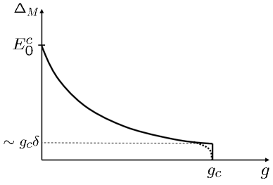
Figure 1: Schematic dependence of the Mott gap on the tunneling conductance $g$ for a periodic granular array of the dimensionality $d>2$. At zero tunneling conductance the Mott gap is given by the charging energy in a single grain and it suppressed exponentially with $g$ for $gz>1.$ The Mott transition takes place at $\Delta_{M}\sim g\delta,$ where $\delta$ is the mean energy level spacing in a single grain. The possible continuous transition that cannot be ruled out at present time is shown by the dotted line.

From Eq. (2) it follows that the Mott gap $\Delta_{M}$ is reduced significantly at the values of the tunneling conductance $gz\sim 1$, where at the same time the perturbation theory becomes unapplicable.

In order to find the Mott gap $\Delta_{M}$ at larger tunneling conductances, we make use of mapping of the original model onto the model of classical charges and construct a mean field theory considering the coordination number $z$ as a large parameter, $z\gg 1$. Within this theory we obtain that the Mott gap $\Delta_{M}$ is exponentially suppressed with the tunneling conductance

$$\Delta_{M}=c\,g\,E^{c}_{0}\;e^{-\pi zg},\;\;\;\;\;\Delta_{M}\gg g\delta\;\;\;\;gz\gtrsim 1,$$ (3)

where $c$ is the number of the order of unity. When deriving equation (3), the nearest neighbor virtual electron tunneling only was taken into account. In the related effective classical model this corresponds to accounting for the short quadruple loops only. For this reason the result (3) holds only as long as the Mott gap $\Delta_{M}$ is larger than the inverse electron escape time from the grain $\Gamma=g\delta$. Solving the inequality $\Delta_{M}>g\delta$ together with the expression for the Mott gap (3) within the logarithmic accuracy we obtain that the later can be used as long as the tunneling conductance $g$ is less than the critical conductance given by the expression

$$g_{c}={1\over{z\pi}}\;\ln(E^{c}_{0}/\delta).$$ (4)

In the regime where the Mott gap $\Delta_{M}$ becomes of the order of the inverse escape time of an electron from a grain $g\delta$ the large loops become important showing tendency to the formation of the metallic state. This means that the value (4) determines the boundary of stability of the insulating state. At the same time the critical tunneling conductance (4) coincides with the boundary of the stability of the metallic phase obtained in Ref. [BLV03, ] meaning that the critical value (4) indeed marks the boundary between the metallic and insulating phases at zero temperature.

Considerations leading to the result (4) for the critical tunneling conductance $g_{c}$ are based on the investigation of the behavior of the system from the insulating and metallic sides implemented in the present paper and Ref. [BLV03, ] respectively. However, both these considerations do not apply in the immediate vicinity of the phase transition. At present the quantitative description of the Mott transition is not available, in particular, the order of the transition remains an open question. Two possible options are illustrated on Fig.1.

Presented description of the Mott transition may not apply in one and two dimensions where even the metallic state $g>g_{c}$ is poorly defined due to divergent Althshuler-Aronov and localization corrections to conductance at $T=0$. The metal to insulator transiton/crossover at higher temperatures, $T>g\delta$ in low dimensional metallic arrays was considered in Refs. [Fazio, ; Jul'ka, ; Glazman, ].

The temperature dependence of the conductivity of granular arrays which are insulators at $T=0$ (i.e. with $g<g_{c}$), is given by the activation law Efetov02

$$\sigma\sim\sigma_{0}\;e^{-\Delta_{M}/T},\hskip 28.45274ptT\ll\Delta_{M},$$ (5)

with $\sigma_{0}$ being the high temperature conductivity as long as the temperature is less than the Mott gap. Indeed, the finite temperature conductivity is due to the electrons and holes that are present in the system as real excitations . Their density is given by the Gibbs distribution that results in the conductivity dependence (5). Note that the expression (5) contains the renormalized Mott gap $\Delta_{M}$ given by Eqs. (2,3).

It is important to note that at finite temperatures the continuous transition between the insulating and metallic phases, is, in fact, rather a crossover than the true phase transition. Indeed, the conductivity at nonzero temperature is finite in both phases, besides the Mott transition does not break any symmetry of the system. However, if the transition is discontinuous at $T=0$ it has to remain discontinuous in some finite temperature interval. In this case the Mott transition would be observable even at nonzero temperature via the jumps of the physical quantities such as conductivity.

The results presented above hold only for periodic arrays. Most of realistic granular/quantum dots arrays contain disorder, in particular, electrostatic disorder.

II.2 Granular arrays with electrostatic disorder

Electrostatic disorder causes fluctuations in electrostatic energy of granules and can thus lift the Coulomb blockade at some sites of a granular sample. This results, in its turn, in the finite density of states at the Fermi level and in appearing the variable range hopping as the dominating mechanism of conductivity. The bare density of states induced by the random potential can be substantially suppressed due to the presence of the long-rang Coulomb interaction as it takes place in semiconductors where the density of states (DOS) is given by the Efros-Shklovskii expression Efros ; Shklovskii

$$\nu_{g}(\varepsilon)\sim(\tilde{\kappa}/e^{2})^{d}\;|\varepsilon|^{d-1},$$ (6)

with $e$ being the electron charge and $\tilde{\kappa}$ being the dielectric constant. This result was recently confirmed in Ref.Ioffe (see also Ref.Pankov ) within the analytic approach of the locator approximation.

In the limit of weak coupling between the grains, $g\ll 1$, the model of granular array can be described in terms of the classical model that deals with the total charges on the grains only

$$H=\sum_{i}\mu_{i}n_{i}+\sum_{ij}n_{i}\;E^{c}_{ij}n_{j},$$ (7)

where $\mu_{i}$ is the random external potential, $n_{i}$ is the electron density on the site $i,$ and $E^{c}_{ij}$ is the Coulomb interaction between the sites $i$ and $j.$ Taking into account the asymptotic behavior of the Coulomb interaction matrix $E^{c}_{ij}\sim e^{2}/r_{ij}\tilde{\kappa},$ where $r_{ij}$ is the distance between the sites $i$ and $j$ and $\tilde{\kappa}$ is the effective dielectric constant in a granular sample we see that the classical model (7) is essentially equivalent to the one studied by Efros and Shklovskii. Therefore their results must be applicable to the model of a granular array (7) as well.

At the same time one expects that the DOS in an array of metallic granules is larger than that in a semiconductor since each metallic grain has a dense electron spectrum. Indeed, one has to remember that there are many electron states in a grain that correspond to the same grain charge while in the model of impurity levels in semiconductors the charge is uniquely (up to the spin) identified with the electron state. The energy of the unoccupied state $\varepsilon_{i}$ in the model (7) is by definition the energy of an electron placed on this state. In the granular metal any state with energy larger than $\varepsilon_{i}$ will be also available for electron placement. Thus, in order to translate ES result (6) to the density of electron spectrum in granular metals one has to integrate the dependence (6) by the energy $\varepsilon$ and multiply it by the bare DOS in a single grain. As a result we obtain

$$\nu(\varepsilon)\sim\nu_{0}\;(|\varepsilon|\tilde{\kappa}/\,e^{2})^{d},$$ (8)

where $\nu_{0}$ is the average DOS in a single grain (measured as the number of states per energy). However, the above expression cannot be used in the Mott argument for the hopping conductivity where one needs to estimate the distance to the first available state $r$ within the energy shell $\varepsilon$ via the relation

$$r^{d}\;\int_{0}^{\varepsilon}d\varepsilon^{\prime}\nu_{g}(\varepsilon^{\prime})\sim 1.$$ (9)

The problem with using the expression for DOS (8) in Eq. (9) is that expression (8) assumes strong correlations of the electron states in the space of the array coordinates. Indeed, expression (8) takes into account the fact that if there is a state available for placement of an electron with a given energy, then, typically on the same grain there will be plenty of other states available for electron placement. But, for application to the hopping conductivity we should not count different electron states that belong to the same grain since it is enough to find at least one to insure the transport. Thus, when finding DOS relevant for the hopping transport the lowest energy states within the each grain are to be count only. We arrive at the conclusion that while in granular metals the electron DOS is modified according to (8), in order to find the distance to the first available state within a given energy shell via Eq.(9), even in granular metals, one has to use the ES expression for DOS in its form (6). Similar considerations were presented in Ref.Shklovskii04 . Following this reference we will call the DOS that counts only lowest excited states in each grain and is relevant for the hopping conductivity by the density of ground states and will denote by a subscript $g$ as in Eq.6.

Apart from the knowledge of the spectrum of electron excitations, description of the hopping conductivity requires understanding the tunneling mechanism of an electron between the two distant grains with energies close to the Fermi level through an optimal chain of other grains where the Coulomb blockade is present. At low temperatures such tunneling process can be realized by means of the virtual electron hopping (cotunneling). As we mentioned in Introduction one has to distinguish the elastic and inelastic cotunneling processes. The elastic cotunneling is the dominant mechanism for hopping conductivity at temperatures $T<\sqrt{E_{0}^{c}\delta}$, while at larger temperatures the electron transport goes via inelastic cotunneling processes.

II.2.1 Hopping via elastic cotunneling

Considering the probability for an electron from the site $i_{0}$ to tunnel to the site $i_{N+1}$ it is convenient to put the Coulomb interaction energy at these sites to zero and count the initial, $\xi_{0}$, and final, $\xi_{N+1}$, electron energies from the Fermi level. The presence of the electrostatic disorder on the grains is modelled by the random potential $\mu_{i},$ such that the energy of the electron (hole) excitation on the site $i$ is

$$E_{i}^{\pm}=E_{i}^{c}\pm\mu_{i}.$$ (10)

The probability $P_{el}$ of a tunneling process via the elastic cotunneling can be easily found for the case of the diagonal Coulomb interaction $E_{ij}^{c}=E^{c}_{i}\,\delta_{ij}$:

$$P_{el}=w\,\bar{g}^{N+1}\,\left({{\bar{\delta}}\over{\pi\bar{E}}}\right)^{N}\delta(\xi_{N+1}-\xi_{0}),$$ (11)

where the factor $w=n(\xi_{0})(1-n(\xi_{N+1}))$ takes into account the occupations $n(\xi_{0})$ and $n(\xi_{N+1})$ of the initial and final states respectively, and the bar denotes the geometrical average of the physical quantity along the tunneling path. For example the average tunneling conductance $\bar{g}$ is defined as

$$\ln\bar{g}={1\over{N+1}}\,\sum_{k=0}^{N}\,\ln g_{k},$$ (12)

where the summation goes over the tunneling path and $g_{k}$ is the tunneling conductance between the $k$-th and $(k+1)$-st grains. The energy $\bar{E}$ is the geometrical average $\ln\bar{E}={1\over{N}}\,\sum_{k=1}^{N}\,\ln\tilde{E}_{k},$ of the following combination of electron and hole excitation energies

$$\tilde{E}_{k}=2\,\left(1/E_{k}^{+}+1/E_{k}^{-}\right)^{-1}.$$ (13)

The presence of the delta function in Eq. (11) reflects the fact that the tunneling process is elastic.

The result (11) for the tunneling probability $P_{el}$ implies that on average the probability falls of exponentially with the distance $s$ along the path: $P_{el}\sim e^{-2s/\xi_{el}}$, where the dimensionless localization length $\xi_{in}$ is given by

$$\xi_{el}={{2}\over{\ln(\,\bar{E}\,\pi/c\bar{g}\,\bar{\delta})}}.$$ (14)

The numerical constant $c$ in the above expression is equal to one for the model of diagonal Coulomb interaction, $E_{ij}^{c}=E^{c}_{i}\,\delta_{ij}$. We show below that the inclusion of the off-diagonal part of the Coulomb interaction results in the renormalization of the constant to some value $0.5\lesssim c<1$.

In a full analogy with the hopping conductivity in semiconductors Shklovskii in the case of granular metals inelastic processes are required to allow an electron to tunnel to a state with higher energy. In granular metals such processes occurs via phonons as well as via the inelastic collisions with other electrons; these proceses are not reflected in the formula (11). Applying the conventional Mott-Efros-Shklovskii arguments, i.e. optimizing the full hopping probability $\propto\exp[-(2s/\xi_{el})-(e^{2}/\tilde{\kappa}Tas)]$, one obtains Eq. (1) for the hopping conductivity with the characteristic temperature

$$T_{\circ}\sim e^{2}/{a\tilde{\kappa}}\,\xi_{el},$$ (15)

where $\tilde{\kappa}$ is the effective dielectric constant of a granular sample, $a$ is the average grain size, and $\xi_{el}$ given by Eq. (14) (when deriving (15) we considered the tunneling path as nearly straight).

In the presence of the strong electric field ${\cal E}$, the direct application of the consideration of Ref. [Shklovskii73, ] for the case of low temperatures ${{T}\over{e\xi_{el}a}}\ll{\cal E}\ll{{\sqrt{\delta E_{\circ}^{c}}}\over{ea}}$ gives the nonlinear current dependence

$$j\sim j_{0}\;e^{-({\cal E}_{\circ}/{\cal E})^{1/2}},$$ (16)

where the characteristic electric field ${\cal E}_{\circ}$ is given by the expression

$${\cal E}_{\circ}\sim T_{\circ}/e\,a\xi_{el}.$$ (17)

The results presented in this subsection are valid as long as the contribution of the inelastic cotunneling to the hopping conductivity can be neglected. This is the case at low temperatures and electric fields $T,{\cal E}ea\ll\sqrt{\delta E_{0}^{c}}.$ Below we present our results for the opposite case where inelastic processes give the main contribution to hopping conductivity.

II.2.2 Hopping via inelastic cotunneling

Inelastic cotunneling is the process where the charge is transferred by means of different electrons on each elementary hop. During such process the energy brought to a grain by incoming electron differs from the energy taken by the outcoming one.

As in the case of elastic cotunneling we assume that the electron tunnels from the grain $i_{0}$ with energy $\xi_{0}$ to the grain $i_{N+1}$ with energy $\xi_{N+1}.$ For the probability of such a tunneling process through a chain of grains in the tunneling path we find the general expression footenote2

$$P_{in}={w\over{4\pi T}}{{\,\bar{g}^{N+1}}\over{\pi^{N+1}}}\left[{{4\pi T}\over{{\bar{E}}}}\right]^{2N}{{|\Gamma(N+{{i\Delta}\over{2\pi T}})|^{2}}\over{\Gamma(2N)}}e^{-{{\Delta}\over{2T}}},$$ (18)

where $\Gamma(x)$ is the Gamma function and $\Delta=\xi_{N+1}-\xi_{0}$ is the energy difference between final and initial states. The appearance of the factor $e^{-\Delta/2T}$ is consistent with the detailed balance principle. Indeed, at finite temperatures an electron can tunnel in both ways with either increase or decrease of its energy. According to the detailed balance principle the ratio of such probabilities must be $e^{\Delta/T},$ that is indeed the case for the function $P_{in}$ (18), since apart from the factor $e^{-\Delta/2T}$ the rest of the equation is even in $\Delta.$

To obtain the expression for the hopping conductivity one has to optimize Eq. (18) with respect to the hopping distance $N$ under the constraint

$$N\,a\,\tilde{\kappa}\,\Delta/e^{2}\sim 1,$$ (19)

following from the ES expression for the density of ground states (6). Optimization of Eq. (18) is a bit more involved procedure than the standard derivation of Mott-Efros-Shklovskii law based on the Gibbs energy distribution function (see Appendix), however it leads to the essentially the same result, i.e. the ES law with

$$T_{0}(T)\sim e^{2}/a\tilde{\kappa}\,\xi_{in}(T),$$ (20)

with the dimensionless localization length $\xi_{in}(T)$ being weakly temperature dependent

$$\xi_{in}(T)={2\over{\ln[\,\bar{E}^{2}/16c\pi T^{2}\bar{g}\,]}},$$ (21)

where the coefficient $c$ equals one for a model with diagonal Coulomb interaction matrix. As in the case of the inelastic cotunneling, the long range interaction result in the reduction of the coefficient to some $1/4\lesssim c<1$.

At zero temperature Eq. (18) for inelastic probability $P_{in}$ for $\Delta<0$ is simplified to

$$P_{in}(T=0)={{w\,2^{2N}\pi}\over{(2N-1)!}}{{|\Delta|^{2N-1}}\over{{\bar{E}}^{2N}}}\left({{\,\bar{g}}\over{\pi}}\right)^{N+1},$$ (22)

while for $\Delta>0$ Eq. (18) gives zero since the process with increase of the energy of the tunneling electron is prohibited at zero temperature.

To obtain the hopping conductivity in the regime of strong electric field $\cal E$ and low temperatures, following Ref. [Shklovskii73, ], we use the condition (19) that defines the distance to the first available electron site within the energy shell $\Delta$ together with equation

$$e{\cal E}r\sim\Delta,$$ (23)

that relates $\Delta$ with the electric filed ${\cal E}$ and the distance between the initial and final tunneling sites $r\sim Na.$ Together Eqs. (19) and (23) define $\Delta\sim\sqrt{{\cal E}e^{3}/\tilde{\kappa}}$ and $N\sim\sqrt{e/\tilde{\kappa}{\cal E}a^{2}}$ that being inserted into Eq. (22) result in the expression for the current

$$j\sim j_{0}\;e^{-({\cal E}_{0}/{\cal E})^{1/2}}.$$ (24a)

where the characteristic electric field $${\cal E}_{0} {\cal E}$$ is a weak function of the applied filed

$${\cal E}_{0}({\cal E})\sim{{e}\over{\tilde{\kappa}\,a^{2}}}\;\ln^{2}[\bar{E}^{2}/e^{2}{\cal E}^{2}a^{2}\bar{g}].$$ (24b)

III The Model

Above presented results were derived within the following model: We consider a $d$-dimensional array of metallic grains. The electron motion within each grain is diffusive and the grains are assumed to be weakly coupled such that the intergranular tunneling conductance $g$ is much less than the intragranule one. The system is described by the Hamiltonian

$$\hat{H}=\hat{H}_{0}+\hat{H}_{c}+\sum_{ij}\,t_{k_{i}k_{j}}^{ij}\,\hat{\psi}^{\dagger}_{i}(k_{i})\;\hat{\psi}_{j}(k_{j}),$$ (25a)

where $$t_{k_{i}k_{j}}^{ij} k_{i} i k_{j} j. \hat{H}_{0} \hat{H}_{c} \mu_{i}$$ is the matrix element representing the electron tunneling amplitude from the state of the grain to the state of the neighboring grain The Hamiltonian in the r. h. s. of Eq. (25a) describes noninteracting isolated disordered grains. The term includes the electron Coulomb interaction and the local external electrostatic potential on each grain

$$\hat{H}_{c}=\sum_{ij}\,\hat{n}_{i}\,E^{c}_{ij}\,\hat{n}_{j}+\sum_{i}\mu_{i}\hat{n}_{i},$$ (25b)

where $E^{c}_{ij}$ is the matrix of Coulomb interaction and $\hat{n}_{i}$ is the operator of electron number in the $i-$th grain. The Coulomb interaction matrix is related to the capacitance matrix in the usual way

$$E^{c}_{ij}=(e^{2}/2)\;C^{-1}_{ij}.$$ (26)

As we discussed in Introduction the random potential $\mu_{i}$ that models the electrostatic disorder removes the Coulomb blockade from some grains.

We let the tunneling elements be random Gaussian variables defined by their correlators:

$$\langle\;t_{k_{1},k_{2}}^{*ij}\,t^{ij}_{k_{1}^{\prime},k_{2}^{\prime}}\;\rangle=t^{2}_{ij}\;\delta_{k_{1}k_{1}^{\prime}}\;\delta_{k_{2}k_{2}^{\prime}},$$ (27)

where $i,j$ are the coordinates of the nearest neighbor grains. The intergranular conductance between the grains $i$ and $j$ is related to average matrix elements as

$$g_{ij}=2\pi\nu_{i}\nu_{j}t_{ij}^{2}$$ (28)

where $\nu_{i}$ is the density of states in the grain $i$. The conductance $g_{ij}$ is defined per one spin component, such that, for example, the high temperature ( Drude ) conductivity of a periodic granular sample is $\sigma=2e^{2}ga^{2-d},$ with $a$ being the size of the grain. In the following we will consider both cases of periodic ( in particular, it means that $\mu_{i}=0,\;\nu_{i}=\nu_{0},\;g_{ij}=g$) and irregular arrays beginning with the former case.

IV Mott gap at small tunneling conductances

In the limit of small tunnelling conductances, $g\ll 1$, and zero temperature a periodic granular array is a charge insulator. The key characteristic of the insulating state is the Mott gap $\Delta_{M}$ in the electron excitation spectrum that can be defined as

$$\Delta_{M}=E_{N=1}-\mu-E_{N=0},$$ (29)

where $\mu$ is the chemical potential, $E_{N=0}$ is the ground state energy of the charge neutral array and $E_{N=1}$ is the minimal energy of the the system with an extra electron added to the neutral state. In the limit of vanishing tunneling conductance, $g\to 0$, the Mott gap $\Delta_{M}$ coincides with the Coulomb energy $E^{c}_{0}\equiv E^{c}_{i,i}$ in a single grain

$$\Delta_{M\,g\to 0}=E^{c}_{0}.$$ (30)

At finite intergranular coupling the Mott gap is reduced as a result of the virtual presence of an electron on the neighboring grains. In the case of weak coupling, $g\ll 1$, the resulting suppression of the Mott gap can be easily calculated within the perturbation theory. The first non vanishing correction appears only in the second order in tunneling matrix elements and can be found with the help of the textbook formula Landau

$$\Delta E=-\sum_{k}{{|V_{k,0}|^{2}}\over{E_{k}-E_{0}}},$$ (31)

where $\Delta E$ is the energy correction to the ground state and the matrix elements of the perturbation $V$ are taken between the ground state $0$ and excited states $k$.

Correction due to finite intergranular coupling should be included in both terms $E_{N=1}$ and $E_{N=0}$ in Eq. (29). The ground state with one extra electron $N=1$ in the limit of zero coupling is degenerate since the extra electron can be present on any grain. Further, we will assume that it occupies grain 1 as it shown in Fig. 2 b. Since we want to find the difference between the corrections to $N=1$ and $N=0$ ground states, it is clear that within the second order perturbation theory in tunneling elements $t_{k_{1},k_{2}}$ only electron hops between grain 1 and its neighbors result in nonzero contribution. All other possible hops give rise to equal corrections to the energies $E_{N=1}$ and $E_{N=0}$ that are mutually cancelled in Eq.(29). Further, since all the neighbors of grain 1 are equivalent, we will consider only electron hops between grain 1 and one of its neighbors that we denote as grain 2. Contribution of the hops between grain 1 and all its other neighbors will simply result in the factor $z$ (coordination number ) in the final answer.

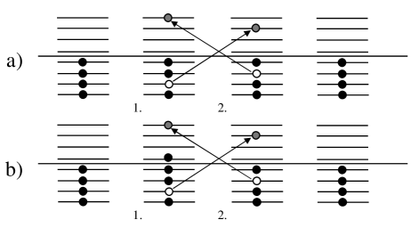
Figure 2: This figure illustrates the virtual electron tunneling processes between neighboring grains that contribute to the reduction of the Mott gap. The tunneling processes shown on figure a) determine the correction to the ground state energy of the charge neutral state $E_{N=0}.$ The correction to the energy of the ground state with one extra electron (placed on grain 1) $E_{N=1}$ is illustrated in figure b).

Now let us consider the correction to the ground state energy $E_{N=0}$. In this case the matrix elements $V_{k,0}$ correspond to the processes of electron tunneling between the neutral neighboring grains. Consider the tunneling process from grain 1 to grain 2 shown in Fig. 2a: The excitation energy of this process is $\varepsilon_{k_{1}}+\varepsilon_{k_{2}}+E_{eh},$ where $\varepsilon_{k_{2}}$ is the bare (with no Coulomb energy included) energy of an electron excitation in grain 2, $\varepsilon_{k_{1}}$ is the bare energy of a hole excitation in grain 1, and $E_{eh}$ is the Coulomb part of the energy of the electron-hole excitation $E_{eh}=E^{c}_{11}+E^{c}_{22}-2E^{c}_{12}$ that for the periodic case under consideration is reduced to

$$E_{eh}=2E^{c}_{0}-2E^{c}_{12}.$$ (32)

The energy correction corresponding to such process is

$$-\Delta E_{N=0}=2\sum_{k_{1},k_{2}}\,{{|t_{k_{1},k_{2}}|^{2}}\over{\varepsilon_{k_{1}}+\varepsilon_{k_{2}}+E_{eh}}},$$ (33)

where the factor 2 takes into account the similar process of electron hopping from grain 2 to grain 1.

Analogously we find the correction to the energy $E_{N=1}$ as illustrated on Fig. 2b: The excitation energy of the process of electron tunneling from grain 2 to grain 1 is $\varepsilon_{k1}+\varepsilon_{k_{2}}+3E^{c}_{11}+E^{c}_{22}-4E^{c}_{12}=\varepsilon_{k_{1}}+\varepsilon_{k_{2}}+2E_{eh}$, while the excitation energy of the process of electron tunnelling from grain 1 to grain 2 is $\varepsilon_{k_{1}}+\varepsilon_{k_{2}}+E^{c}_{11}-E^{c}_{22}=\varepsilon_{k_{1}}+\varepsilon_{k_{2}}.$ The corresponding correction to the energy $E_{N=1}$ reads

$$-\Delta E_{N=1}=\sum_{k_{1},k_{2}}\,{{|t_{k_{1},k_{2}}|^{2}}\over{\varepsilon_{k_{1}}+\varepsilon_{k_{2}}+2E_{eh}}}+{{|t_{k_{1},k_{2}}|^{2}}\over{\varepsilon_{k_{1}}+\varepsilon_{k_{2}}}}.$$ (34)

One can see that corrections (33, 34) are ultraviolet divergent. However, their difference must be finite since it represents the measurable quantity - correction to the Mott gap. It is, indeed, the case: Subtracting Eq. (33) from Eq.(34), presenting summation over states as integrals $\varepsilon_{k_{1}(k_{2})}\to\varepsilon_{1(2)}$ and introducing further the variable $\varepsilon=\varepsilon_{1}+\varepsilon_{2}$ we obtain

$$\Delta_{M}-E^{c}_{0}=z\nu_{0}^{2}t^{2}\int_{0}^{\infty}\varepsilon\,d\varepsilon\left[{1\over{\varepsilon+2E_{eh}}}-{2\over{\varepsilon+E_{eh}}}+{1\over{\varepsilon}}\right],$$

where $\nu_{0}$ is the density of states in a single grain and $t^{2}$ defined by Eq.(27) appears from the averaging over matrix elements. Taking the integral in the above expression we obtain the result (2).

In the derivation of the reduction of the Mott gap presented in this section we neglected the fact that an extra electron added to the neutral system in the presence of finite intergranular coupling can move diffusively over the sample. Contributions corresponding to such processes, as we will see below, are suppressed by an extra small factor $\delta/E_{0}^{c}\ll 1$ and, thus, can be neglected.

V Phase and charge representations

The perturbation theory presented in Sec. IV is limited to the regime of low tunneling conductance $g\ll 1$. Moreover, the high order tunneling processes that are very important for understanding the physics of Mott transition and hopping conductivity cannot be included in this way. For this reason one has to seek for a convenient approach applicable at intermediate tunneling conductances and capable of description of the effects of high order tunnelling processes. In this view, a useful tool in approaching this problem is the phase functional approach AES that allows further mapping of the system to the Coulomb gas of charged particles in d+1 dimensions Schmid ; Zaikin .

V.1 Phase representation

The phase functional approach is based on the decoupling of the Coulomb interaction term  (25b) in the Hamiltonian (25a) by means of the the potential field $V(\tau)$ that is further absorbed into the gauge transformation of the fermionic fields

$$\psi_{i}(\tau)\to\psi_{i}(\tau)\,e^{-i\,\phi_{i}(\tau)},\;\;\;\;\;\phi_{i}(\tau)=\int_{-\infty}^{\tau}V_{i}(\tau^{\prime})d\tau^{\prime}.$$ (35)

Since the action of an isolated grain is gauge invariant the phases $\phi_{i}(\tau)$ enter the whole lagrangian of the system only through the tunnelling matrix elements

$$t_{ij}\to t_{ij}\,e^{i\phi_{ij}(\tau)},$$ (36)

where $\phi_{ij}(\tau)=\phi_{i}(\tau)-\phi_{j}(\tau)$ is the phase difference of the $i-$th and $j-$th grains.

A simple description in terms of phase variables can be obtained via integrating out the fermionic fields and expanding the resulting rather complicated action to the lowest non vanishing order in tunneling elements. As a result one obtains the Ambegaokar, Eckern, Schön (AES) action AES

$$S_{AES}=-{1\over{2e^{2}}}\sum_{ij}\int d\tau\,(\dot{\phi}_{i}+i\mu_{i})\,C_{ij}\,(\dot{\phi}_{j}+i\mu_{j})+S_{t}[\phi],$$ (37a)

where the tunneling term $$S_{t}$$ at zero temperature is

$$S_{t}[\phi]={1\over{2\pi}}\sum\limits_{<ij>}g_{ij}\int\limits_{-\infty}^{+\infty}\,d\tau_{1}\,d\tau_{2}{{e^{i\phi_{ij}(\tau_{1})-i\phi_{ij}(\tau_{2})}}\over{(\tau_{1}-\tau_{2})^{2}}},$$ (37b)

where the angular brackets mean summation over the nearest neighbors. The higher order terms in the expansion of the total action in the tunneling matrix elements cannot be always neglected and, in general, must be taken into account along with the nearest neighbor action (37). However, before considering these more complicated higher order terms, it is instructive to analyze, first, the action (37) in details. Moreover, as we will show, even at $T=0$ there is a regime where the AES action is applicable. We, thus, proceed to the description of the charge mapping beginning with the AES action, and later, in Sec. VIII, we will show how the higher order tunneling terms can be included into the mapping. Also, for simplicity, we will first consider the case of the regular periodic array.

V.2 Charge representation

Proceeding to the mapping of the action (37) onto the model of the classical Coulomb gas and using the method of Ref. [Schmid, ], we first expand the partition function $Z$ to all orders in the tunneling part of the action $S_{t}$

$$Z=Z_{0}\,\sum_{N=1}^{\infty}\,\langle\;S_{t}^{N}[\phi]\;\rangle\,/\,N!\,.$$ (38)

Here $Z_{0}$ is the partition function of a system of isolated grains and the angle brackets assume averaging with respect to the Coulomb phase action that for the case $\mu_{i}=0$ under consideration reads

$$S_{c}=-{1\over{2e^{2}}}\sum_{ij}\int d\tau\,\dot{\phi}_{i}\,C_{ij}\,\dot{\phi}_{j}.$$ (39)

On the next step, for each term in the expansion (38) we write the $N$-th power of the tunnelling action $S_{t}$ explicitly as the product

$$S_{t}^{N}[\phi]=\prod_{n=1}^{N}\,S_{t}^{(n)},$$ (40a)

where the index $$n S_{t}$$ of the tunneling action reminds that the time integrations in each term in the above product are independent

$$S_{t}^{(n)}={{g}\over{2\pi}}\sum\limits_{<ij>}\int\limits_{-\infty}^{+\infty}\,{{d\tau_{n}\,d\tau_{n}^{\prime}}\over{(\tau_{n}-\tau_{n}^{\prime})^{2}}}\;e^{i\phi_{ij}(\tau_{n})-i\phi_{ij}(\tau_{n}^{\prime})}.$$ (40b)

Writing the powers of the tunneling action as products (40a) allows to implement the integrations over the phase fields $\phi_{i}(\tau)$ exactly for each term in the expansion (38) with the help of the formula

$$\left\langle e^{i\sum_{n}\phi_{i}(\tau_{n})e_{n}}\right\rangle=e^{-U^{c}},$$ (41)

where $U^{c}$ given by the expression

$$U^{c}={1\over 2}\sum_{n_{1},n_{2}}E^{c}_{i_{n_{1}}i_{n_{2}}}|\tau_{n_{1}}-\tau_{n_{2}}|\,e_{n_{1}}\,e_{n_{2}},$$ (42)

can be viewed as a Coulomb energy of a system of classical charges in a space with an extra time dimension temperature .

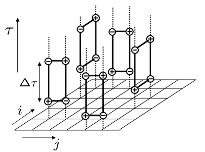
Figure 3: Illustration of the mapping of a quantum granular array model in the nearest neighbor hopping approximation onto the classical model of gas of quadruples in $d+1$ dimensions.

The classical charges $e_{n}=\pm 1$ interact via the 1d Coulomb potential along the time direction while the strength of the interaction is given by the “real” Coulomb energy of original quantum electrons $E^{c}_{ij}.$

From Eq. (40b) we see that each tunneling term $S_{t}^{(n)}[\phi]$ contains the sum of four phase fields in the exponent

$$i\phi_{i}(\tau_{n})-i\phi_{j}(\tau_{n})-i\phi_{i}(\tau_{n}^{\prime})+i\phi_{j}(\tau_{n}^{\prime}).$$ (43)

Each of these fields, according to Eqs. (41,42), gives rise to a classical charge located at coordinates corresponding to the arguments of the phase fields. This means that the classical charges appear as quadruples that occupy only the neighboring sites as it is shown in Fig. 3.

The time dependent kernel in Eq.(40b) can be written in the form

$${{g}\over{2\pi}}\;{1\over{(\tau_{n}-\tau^{\prime}_{n})^{2}}}=e^{-{\cal U}^{q}_{n}(\tau_{n}-\tau^{\prime}_{n})},$$ (44)

such that ${\cal U}^{q}_{n}$ defines the ”internal” energy of $n-$th quadruple

$${\cal U}^{q}_{n}=\ln[2\pi(\Delta\tau_{n})^{2}/g],$$ (45)

with $\Delta\tau_{n}$ being the size of the $n-$th quadruple in the $\tau-$ direction as shown in Fig. 3.

Thus, the partition function, Eq. (38), of the quantum problem under consideration in the nearest neighbor electron tunneling approximation can be presented as a partition function of classical charges that appear in quadruples all charges being subject to the Coulomb interaction (42). The total energy of the system of N quadruples can be written as

$$U^{q}=\sum_{n=1}^{N}{\cal U}^{q}_{n}+U_{4N}^{c},$$ (46)

where ${\cal U}^{q}_{n}$ is the internal energy of the $n-$th quadruple and $U_{4N}^{c}$ is the Coulomb energy of 4N charges that form N quadruples defined by Eq. (42). We notice that different quadruples interact with each other only via the Coulomb part of the energy $U^{c}.$

In the following sections we will consider the thermodynamic properties of the classical model and set correspondence between the parameters of the original quantum model and the effective classical one.

VI Thermodynamics of the classical model in the limit of low quadruple density

The thermodynamic potential $\Omega$ of the classical model (46) can be found in the limit of the low quadruple density that, as we will show below, corresponds to the case of the low tunneling conductance $g\ll 1$ in the quantum model. In this limit one can neglect the mutual interaction of deferent quadruples considering them as free independent objects and the thermodynamic potential $\Omega$ of the whole system is reduced to the sum of the free energy ${\cal F}_{0}$ of a single quadruple multiplied by the number of the quadruples $N$ and the entropy $S$ of the quadruple configuration space

$$\Omega=N{\cal F}_{0}-S.$$ (47)

The entropy of $N$ independent quadruples is given by the expression

$$S=N\ln V-\ln N!,$$ (48)

where $V=LM$ is the volume of the $d+1$ dimensional system with L being the size of the system in $\tau-$ direction and $M$ being the total number of the sites (grains) in the array. The term $\ln N!$ in Eq. (48) appears from the term $1/N!$ in the expansion (38). In the classical statistical mechanics such term appears due to equivalence of the classical configurations that differ only by mutual permutations of particles. Thus, in the thermodynamic limit $N\to\infty$ for the thermodynamic potential $\Omega$ in the case of low quadruple density we obtain the expression

$$\Omega=N{\cal F}_{0}+N\ln\rho-N,$$ (49)

where $\rho=N/V$ is the density of quadruples in $d+1$ dimensions.

The partition function of a single quadruple is given by the expression

$${\cal Z}_{0}={g\over{\pi}}\,\int_{0}^{\infty}{{d\tau}\over{\tau^{2}}}\,e^{-E_{eh}\,\tau},$$ (50)

where the energy of the electron-hole excitation is defined by Eq.(32). Equation (50) is divergent on low integration limit and in order to regularize it we introduce the time cut-of $\lambda$ obtaining ${\cal Z}_{0}=g/\pi\lambda$ so that the free energy of a single quadruple ${\cal F}_{0}=-\ln{\cal Z}_{0}$ becomes

$${\cal F}_{0}=-\ln(g/\pi\lambda).$$ (51)

VI.1 Density of classical charges

The thermodynamic potential given by Eqs.(49,51) determines all the thermodynamic quantities of the classical model in the limit of low quadruple density. In particular, the density itself can be obtained via minimization of $\Omega$ with respect to the number of quadruples $N$ resulting in

$$\rho=g/\pi\lambda.$$ (52)

We would like to note that the obtained density coincides with the single quadruple partition function $\rho={\cal Z}_{0}.$ The result for the density $\rho$ (52) can be better understood considering a discrete time axis. In this case the cut-of distance $\lambda$ would be the distance between the neighboring sites in $\tau-$ direction and the dimensionless density according to Eq. (52) would be $g/\pi.$ Thus, it becomes clear that the limit of low conductance $g\ll 1$ corresponds to the limit of the low occupation number of classical charges.

VI.2 Relation between the Mott gap and dielectric constant of classical gas

In order to make the developed mapping useful one has to express the physical observables of the original quantum model in terms of the corresponding thermodynamic quantities of the classical model. Below we show that the key characteristic of the insulating state - the Mott gap $\Delta_{M}$ is related to the dielectric constant $\kappa_{\tau}$ of the effective classical model measured in the direction of $\tau-$ axis as

$$\Delta_{M}=E_{0}^{c}/\kappa_{\tau}.$$ (53)

To prove relation (53) we first note that the gap $\Delta_{M}$ in the electron spectrum determines the asymptotic behavior ( $\tau\to\infty$ ) of the single electron Green function

$$G_{ii}(\tau)\sim e^{-\Delta_{M}\,|\tau|}.$$ (54)

At the same time the asymptotic behavior of the Green function $G_{ii}(\tau)$ with exponential accuracy coincides with the asymptotic behavior of the phase correlation function

$$G_{ii}(\tau_{1}-\tau_{2})\sim\Phi(\tau_{1}-\tau_{2})\equiv\langle\,e^{i\phi_{i}(\tau_{1})-i\phi_{i}(\tau_{2})}\,\rangle,$$ (55)

where the angular brackets stand for averaging with respect to the phase functional (37), written explicitly

$$\Phi(\tau_{1}-\tau_{2})=Z^{-1}\,\int D[\phi]\;e^{i\phi_{i}(\tau_{1})-i\phi_{i}(\tau_{2})}\,e^{S[\phi]}.$$ (56)

All the considerations that was previously used in order to derive the effective model (46) can be applied to the correlation function (56) as well. Repeating all the necessary steps we notice that phases $\phi_{i}(\tau_{1})$ and $\phi_{i}(\tau_{2})$ that enter the exponent in Eq.(56) result in appearance of two external charges of opposite signs located on the site i at time coordinates $\tau_{1}$ and $\tau_{2}.$ Further, we see that the phase correlation function $\Phi$ is related to the thermodynamic potential of the system with two external charges $\Omega_{2}(\tau_{1}-\tau_{2})$ as

$$\Phi(\tau)=e^{-\Omega_{2}(\tau)}.$$ (57)

The function $\Omega_{2}(\tau)$ is normalized such that $\Omega_{2}(0)=0.$ The function $\Omega_{2}$ is nothing but effective interaction of two external charges in the presence of quadruples. The initial electrostatic interaction is reduced in the presence of quadruples and the asymptotic behavior of the function $\Omega_{2}$ takes the form

$$\Omega_{2}(\tau)=|\tau|\,E^{c}_{0}/\kappa_{\tau},\;\;\;\;\;\;\;\tau\to\infty,$$ (58)

where $\kappa_{\tau}$ is the dielectric constant. This proves the relation between the Mott gap and dielectric constant of the classical Coulomb gas in $\tau-$ direction (53 ).

VI.3 Mott gap in the limit of $gz\ll 1$

Finally, in order to better understand the relationship between the original quantum model and the effective classical one we will rederive the result (2) for the Mott gap in the case of small tunneling conductance $gz\ll 1$ within the framework of the effective classical model.

Let us consider two charges $e_{1}$ and $e_{2}$ ( see Fig. 4 ) of the opposite signs located on the site $i$ at time coordinates $\tau_{1}$ and $\tau_{2}$ respectively. In the absence of surrounding quadruples their interaction energy would be $E^{c}_{0}|\tau_{1}-\tau_{2}|$ that gives the zero-order value of the Mott gap $\Delta_{M}=E^{c}_{0}.$ The bare interaction energy $E^{c}_{0}$ of two charges is reduced due to the presence of quadruples. In order to find this reduction it is convenient to consider the electric field created by the charge 1 and partially screened by the surrounding quadruples at the point $\tau_{2}$ of location of charge 2. In the limit of low quadruple density the screening of the interaction due to different quadruples can be considered independently.

It is easy to see that the electric field at the point $\tau_{2}$ is affected by the presence of the quadruple only if the later is placed such that charge $e_{2}$ is inside the quadruple as it is shown in Fig. 4. Depending on the arrangements of quadruple charges one can distinguish two different situations shown in Fig. 4 a) and b). In the case a) the electric field that charge $e_{2}$ feels is

$$E^{(a)}=-3E^{c}_{0}+2E^{c}_{12}=-E^{c}_{0}-E_{eh},$$ (59a)

while in the case b) it is

$$E^{(b)}=E^{c}_{0}-2E^{c}_{12}=-E^{c}_{0}+E_{eh}.$$ (59b)

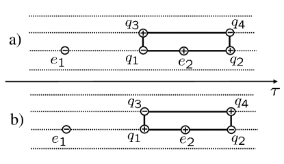
Figure 4: An electric filed that charge $e_{2}$ feels consists of the field created by the charge $e_{1}$ and the fields created by the charges of the quadruple $q_{1},...q_{4}.$

We see from Eqs. (59) that the electric field at the point $\tau_{2}$ of location of charge 2 gets an additional contribution $\pm E_{eh}$ depending on the arrangements of quadruple charges. The probability of the configuration a) is given by the Gibbs weight as

$$P_{a}(\tau_{q_{1}},\tau_{q_{2}})={\cal Z}_{0}^{-1}e^{-{\cal U}^{q}(\tau_{q_{2}}-\tau_{q_{1}})-E_{eh}(\tau_{q_{2}}-\tau_{q_{1}})+\tau_{q_{1}}E_{eh}},$$

where the time coordinates of quadruple charges $\tau_{q_{1}}$ and $\tau_{q_{2}}$ are taken with respect to coordinate $\tau_{2}$ where charge $e_{2}$ is located such that $\tau_{q_{2}}>0$ and $\tau_{q_{1}}<0.$ Analogously we find the probability of the configuration b)

$$P_{b}(\tau_{q_{1}},\tau_{q_{2}})={\cal Z}_{0}^{-1}\,e^{-{\cal U}^{q}(\tau_{q_{2}}-\tau_{q_{1}})-E_{eh}(\tau_{q_{2}}-\tau_{q_{1}})-\tau_{q_{1}}E_{eh}}.$$

The probabilities $P_{a}$ and $P_{b}$ must be further multiplied by the quadruple density $\rho,$ coordination number $z$ and combinatoric factor 2. Multiplication by $\rho$ simply cancels the factor ${\cal Z}_{0}^{-1}$ due to the relation $\rho={\cal Z}_{0}$ that we pointed out below Eq.(52). The additional contribution to the electric field at coordinate $\tau_{2}$ of charge 2 due to the presence of the quadruples becomes

$$\Delta E=2zE_{eh}\int_{-\infty}^{0}d\tau_{q1}\int_{0}^{\infty}d\tau_{q_{2}}\;(P_{b}-P_{a}).$$ (60)

The dielectric constant $\kappa_{\tau}$ is given by the expression $\kappa_{\tau}^{-1}=(E^{c}_{0}-\Delta E)/E^{c}_{0}.$ Taking integrals in Eq. (60) we finally get the dielectric constant

$$\kappa_{\tau}^{-1}=1-{{2gz}\over{\pi}}\,{{E_{eh}}\over{E_{0}^{c}}}\,\ln 2,$$ (61)

that taking into account relation (53) between the Mott gap and dielectric constant is indeed consistent with result (2) previously obtained within the direct perturbation theory in tunneling matrix elements.

VII Mott gap at large tunneling conductances

In this section we continue our investigation of the quadruple model (46) now coming to the regime of moderately large tunneling conductance $gz\geq 1.$ We show that within this model the Mott gap $\Delta_{M}$ is exponentially reduced with growth of $g$ but nevertheless it always remains finite and, thus, the quantum system represented by the model  (46) is always an insulator at $T=0$ even at arbitrary large tunneling conductance $g.$ This statement, however, turns out to be an artifact of neglecting the high order tunnelling terms in derivation of the phase action (37) and the following from it model (46). Below we show that models (37,46) are applicable as long as the Mott gap $\Delta_{M}$ is larger than the inverse escape time of an electron from a grain $\Gamma=g\delta.$ Thus, the results of this section are applicable as long as the obtained Mott gap $\Delta_{M}$ is larger than the inverse escape time $g\delta.$

VII.1 Mean field approximation

The model (46) can hardly be solved in general case and further in this section we make two assumptions that will allow us to construct a mean field approachHerrero . Namely,

(i) we take the diagonal matrix of Coulomb interaction $E^{c}_{ij}=E^{c}_{0}\,\delta_{ij}.$

(ii) we assume that the coordination number $z$ is large.
These two assumptions allow to reduce the quadruple problem in $d+1$ dimensions to the problem of one dimensional dipoles with self consistent dipole interaction.

To construct a mean filed theory let us pick up a site $i$ and consider the influence of the neighboring sites on it in a mean field manner. The quadruple that occupies the site $i$ and a neighboring site $j$ is reduced to the dipole located on the site $i.$ The mutual interaction of two charges of the resulting dipole consists of the quadruple interaction ${\cal U}^{q}$ and of the Coulomb interaction energy of quadruple charges located at the site $j.$ The later must be taken into account in a self-consistent way. The mutual influence of the neighboring sites due to direct Coulomb interaction is absent due to our choice of the diagonal Coulomb matrix $E^{c}_{ij}.$ Thus the internal dipole interaction energy becomes

$${\cal U}_{d}=\ln[\pi(\Delta\tau_{n})^{2}/gz]+\Omega_{2}(\Delta\tau_{n}),$$ (62)

where the interaction energy $\Omega_{2}(\tau)$ of two external charges must be calculated self consistently in terms of the dipole model. The asymptotic behavior of this function at the same time according to Eq. (58) determines the dielectric constant $\kappa_{\tau}$ that is directly related to the Mott gap $\Delta_{M}$ of the original model.

Thus we arrive at the simplified one dimensional model of dipoles bounded by the internal interaction (62). Apart from the bounding interaction all charges are subject to the 1-d Coulomb interaction

$$U^{c}_{1d}={E^{c}_{0}\over 2}\sum_{n_{1},n_{2}}|\tau_{n_{1}}-\tau_{n_{2}}|\,e_{n_{1}}\,e_{n_{2}}.$$ (63)

In the limit of large density $\rho\gg 1$ that corresponds to the case of large tunneling conductance $g\gg 1$ the Coulomb interaction gets sufficiently screened. For this reason the expression for the density (52) as well as the identity ${\cal Z}_{0}=\rho_{0}$ are applicable in the dense limit too. In the dense limit the screening effects can be usually well described within the Debay theory:

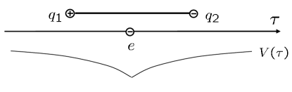
Figure 5: Screening of the external charge $e$ in the dipole model. The Coulomb potential of the charge $e$ is screened by the dipole charges $q_{1}$ and $q_{2}$ resulting in the effective screened potential $V(\tau).$

Consider the charge $e$ placed at $\tau=0$ shown in Fig. 5. The Coulomb potential of this charge screened by the dipole charges obeys the Poisson equation

$$\partial_{\tau}^{2}V(\tau)=-2E^{c}_{0}\;(q(\tau)-\delta(\tau)),$$ (64)

where $q(\tau)$ is the average density of all dipole charges and $\delta(\tau)$ is the delta function. At the same time the density of dipole charges is given by the Gibbs distribution: The contribution of two charges $q_{1}$ and $q_{2}$ of a single dipole ( located at coordinates $\tau_{1}$ and $\tau_{2}$ respectively ) to the charge density $q(\tau)$ is

$${\cal Z}_{0}^{-1}[\delta(\tau-\tau_{1})-\delta(\tau-\tau_{2})]\,e^{-\tilde{\cal U}_{d}(\tau_{1}-\tau_{2})-V(\tau_{1})+V(\tau_{2})},$$ (65)

where the energy $\tilde{\cal U}_{d}(\tau)$ that enters the Gibbs exponent includes the dipole interaction energy ${\cal U}_{d}(\tau)$ and the screened Coulomb interaction of charges $q_{1}$ and $q_{2}$

$$\tilde{\cal U}_{d}(\tau)={\cal U}_{d}(\tau)+\Omega_{2}(\tau).$$ (66)

We note that within the approximation that we use the screened potential $V(\tau)$ is nothing but the effective screened interaction of two charges $\Omega_{2}(\tau)$ so that

$$V(\tau)=\Omega_{2}(\tau).$$ (67)

Multiplying Eq. (65) by the dipole density $\rho,$ making use of the identity ${\cal Z}_{0}=\rho$ and integrating over the coordinates $\tau_{1},\tau_{2}$ we obtain the averaged charge density

$$q(\tau)={{2gz}\over{\pi}}\,\int\limits_{-\infty}^{\infty}d\tau^{\prime}\,{{e^{-2V(\tau-\tau^{\prime})}}\over{(\tau-\tau^{\prime})^{2}}}\sinh[V(\tau^{\prime})-V(\tau)].$$ (68)

Equations (64) and (68) form a closed system of equations that determine the potential $V(\tau).$ In the next subsection we present the solution of these equations.

VII.2 Solution of the mean field equations

Numerical solution of Eqs. (64,68) for moderately large tunneling conductances $gz\gtrsim 1$ shows that the external charge is never screened completely and the long time asymptotic behavior of the function $V(\tau)$ in Eq. (67) has a linear form

$$V(\tau)=|\tau|E^{c}_{0}\,\kappa_{\tau}^{-1}\,,\;\;\;\;\;\tau\to\infty,$$ (69)

where the inverse dielectric constant $\kappa_{\tau}^{-1}$ becomes very small for large conductances but nevertheless it remains finite. The numerical solution also shows that the potential $V(\tau)$ behaves logarithmically on intermediate time scales and then turns to the insulating linear behavior (69) on longer times (crossover scale is given below). This suggests the following analytic approach to the solution of mean field Eqs. (64,68): To find the potential $V(\tau)$ on intermediate times where nonlinear effects are not important we consider Eq. (68) in the linear approximation with respect to $V(\tau)$. As a result in the Fourier representation we obtain

$$q_{\omega}=-2zg|\omega|V_{\omega}.$$ (70)

Together with the Poisson equation (64) written in the Fourier representation $-\omega^{2}V(\omega)=-2{E}^{c}_{0}\,(q_{\omega}-1)$ equation (70) defines the potential

$$V_{\omega}=-{1\over{\omega^{2}/2{E}^{c}_{0}+2zg|\omega|}},$$ (71)

that being transformed to the time representation for $\tau>(E^{c}_{0}g)^{-1}$ results in

$$V(\tau)={{\ln(\tau E^{c}_{0}g)}\over{2\pi zg}}.$$ (72)

The linear approximation that we used in Eq. (68) is valid as long as the potential $V(\tau)$ is small. This assumes that dependence (72) is applicable for not very long times $\tau\ll\exp(\pi zg)/gE_{0}^{c}.$ From the logarithmic form of the answer (72) it follows that the change in the charging energy

$$E_{0}^{c}\to\xi\,E_{0}^{c}$$ (73)

in Eq. (72) results in a constant shift of the potential $V(\tau)\to V(\tau)+(1/2\pi zg)\,\ln\xi.$ At the same time the only term in Eq. (68) that is sensitive to this shift is the potential $V(\tau)$ in the exponent that provides the renormalization of conductance

$$g\to g-(1/\pi z)\ln\xi.$$ (74)

This consideration allows to solve the system of Eqs. (64,68) for the case of large tunnelling conductance in the renormalization group(RG) scheme. Since the charging energy $E_{0}^{c}$ is the only energy scale in the problem, the scaling of this energy with conductance determines the scaling of the Mott gap. Thus, from the scaling Eqs. (73,74) we finally obtain the expression for the Mott gap (3).

Equation (3) agrees with the result of RG approach of Ref. [Universal, ] where the opening of the Mott gap $\Delta_{M}$ was assumed to happen at the point where the tunneling conductance running under RG scheme flowed to values of the order one. We would like to note that the present approach does not rely on any assumptions of this kind: we first apply the RG scheme to reduce the conductance to values $gz\geq 1,$ and further we solve the equation numerically and show that opening of the gap indeed takes the place, i.e. the asymptotics of the potential $V(\tau)$ has a linear form indeed.

VIII Inclusion of higher order tunnelling terms

So far we considered the quadruple model (46) that includes only the nearest neighbor electron tunnellings. In the present section we describe how the high order tunneling terms can be included into our mapping scheme and in the following sections we apply this technique to the problem of hopping conductivity and Mott transition in granular arrays.

Keeping in mind the applications to the irregular arrays, as in the case of hopping conductivity, in this section we include the random on-site potential $\mu_{i}$ in the Hamiltonian into consideration. Also we take into account variations of tunneling conductance $g$ from grain to grain as well as variations of charging energies $E^{c}_{i}$ and the mean energy level spacings $\delta_{i}.$

In order to construct the effective classical model that takes into account higher order tunnelling terms we proceed in the same way as in the derivation of AES functional Eqs. (37). First we decouple the Coulomb interaction term in Eq. (25a) with the help of potential field $V(\tau)$

$${\cal L}_{c}=-{1\over{2e^{2}}}\,\sum_{ij}[V_{i}+i\mu_{i}]\,C_{ij}\,[V_{j}+i\mu_{j}]-i\sum_{i}n_{i}V_{i},$$ (75)

where $n_{i}=n_{i}(\tau)$ is the electron density field. The term $-in_{i}V_{i}$ can be absorbed by the fermion gauge transformation given by Eqs. (35) such that the action that governs dynamics of the potential field $V(\tau)$ becomes

$${\cal L}_{c}=-{1\over{2e^{2}}}\,\sum_{ij}[V_{i}+i\mu_{i}]\,C_{ij}\,[V_{j}+i\mu_{j}].$$ (76)

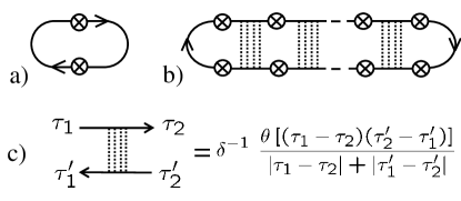
Figure 6: Diagram a) represents the lowest order correction in tunneling conductance $g$ to the partition function, the first term in the expansion (38). The solid lines denote the propagator of electrons, the crossed circles stand for the phase dependent tunnelling matrix elements $t_{ij}e^{i\phi_{ij}(\tau)}.$ Diagram b) describes a higher order correction in tunnelling matrix elements $t_{ij}.$ The dotted lines represent impurity scattering. The diagram c) shows the zero dimensional diffusion in time representation.

Further, following Ref. [Beloborodov01, ] we proceed with diagrammatic expansion of the partition function $Z$ in tunnelling matrix elements $t_{ij}\,e^{i\phi_{ij}(\tau)}$. In the lowest order we reproduce the results obtained within the phase functional. Indeed, the lowest order correction to the partition function $Z$ shown in Fig. 6a simply results in the first term in the expansion (38). All disconnected diagrams of the type shown in Fig. 6a must also be included in the partition function, this reproduces all high order terms in the expansion (38). Integration over the phase fields $\phi_{i}(\tau)$ can be implemented exactly as it was described in Sec. V.2 resulting in the appearance of classical charges in $d+1$ dimensions with the Coulomb interaction energy

$$U={1\over 2}\sum_{n_{1},n_{2}}E^{c}_{i_{n_{1}}i_{n_{2}}}|\tau_{n_{1}}-\tau_{n_{2}}|\,e_{n_{1}}\,e_{n_{2}}+\sum_{n}\mu_{i_{n}}\tau_{n}e_{n}.$$ (77)

that differs from Eq. (42) only by the presence of the random potential $\mu_{i}$ not previously taken into account.

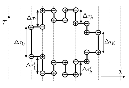
Figure 7: Illustration of the mapping of the model of quantum electrons in a granular array onto the model of classical charges imbedded into the electron world lines forming loops. The illustration is shown for the case of $1+1$ dimensions ($1d$ granular array), generalization to higher $d+1$ dimensions is straightforward.

Thus, inclusion of all disconnected diagrams, Fig. 6a, and their further averaging over the phases reproduces the classical quadruple model (46). The expression for the internal quadruple energy for the case where conductance $g$ varies from contact to contact is the straightforward generalization of Eq. (45)

$${\cal U}^{q}_{n}=\ln[2\pi(\Delta\tau_{n})^{2}/g_{ij}].$$ (78)

The advantage of the mapping of the original quantum model on the classical electrostatic system is that it allows to include the higher order tunneling processes shown in Fig. 6b in essentially the same way as the nearest neighbor hoppings. The higher order diagrams include the single grain diffusion propagator

$$D_{0}=2\pi\delta^{-1}/|\omega_{1}-\omega_{2}|,$$ (79)

that being transformed into the time representation results in the expression shown in Fig. 6c. Each tunneling matrix element in the diagram Fig. 6b includes the phase variables as $t_{ij}e^{i\phi_{ij}(\tau)}.$ This allows to present the diagram in Fig. 6b as a charge loop shown in Fig. 7. The charges interact electrostatically and are subject to the local potentials according to Eq. (77). The internal energy of a single $K-$th order loop is

$$E^{(K)} = \ln[2\pi K/g_{0}]-\sum_{k=1}^{K-1}\ln[g_{k}\delta/2\pi]+\ln|\Delta\tau_{0}|$$ (80)

$$+\ln|\Delta\tau_{K}|+\sum_{k=1}^{K-1}\ln(|\Delta\tau_{k}|+|\Delta\tau_{k}^{\prime}|),$$

where the time intervals $\Delta\tau_{k}$ and $\Delta\tau^{\prime}_{k}$ shown in Fig. 7 are restricted to have opposite signs, i.e. $\Delta\tau_{k}\Delta\tau^{\prime}_{k}<0.$

We mapped the model of quantum electrons in a metallic array with Coulomb interaction onto the classical model of Coulomb charges bounded by the electron world lines and forming loops. First order loops that form quadruples represent the process of virtual electron tunnelings to the neighboring grains and back. Higher order loops represent electron motion on larger distances.

In the Mott insulator state electrons cannot move on large distances. This assumes that in the classical representation of the Mott insulator state the thermodynamics of the classical charges will be dominated by the contribution of the short loops, while high order loops will be energetically suppressed.

In the metallic state, on the contrary, diffusive motion of electrons on any distances is possible meaning that in the classical model the loops of infinite order are present. It is clear that the insulator to metal transition in terms of the classical model corresponds to the transition at which the infinite loops that were suppressed in the insulating state begin to proliferate. Infinite loops represent almost free charges that screen the Coulomb interaction. The inverse dielectric constant $\kappa_{\tau}^{-1}$ of this state is zero that corresponds to the absences of the Mott gap $\Delta_{M}$.

The detailed description of the Mott transition is difficult since it requires the analysis of contribution of high order loops in the regime where the tunneling conductance $g$ is not small and the Mott gap $\Delta_{M}$ is already strongly reduced due to the quadruple screening according to Eq. (3). Such description, on the qualitative level is performed in Sec. X, while in the next section we will study the high order electron tunnellings in a more simple regime of low tunneling conductance. As we discussed above, the high order tunnelings being not important for the thermodynamics in the regime of small $g$ are crucial for the description of the hopping transport in the case of irregular array.

IX Hopping conductivity in Granular metals

In Sec. VIII it was shown that the periodic granular array with low tunneling conductances $g$ is the Mott insulator with the hard gap $\Delta_{M}$ in the electron excitation spectrum. This assumes the activation conductivity behavior, $\sigma\sim\exp{(-\Delta_{M}/T})$, and excludes the possibility of hopping transport. However, as we pointed out in the Introduction, in realistic granular arrays there are many reasons for electrostatic disorder that compensates the Coulomb blockade on some sites. This gives rise to the finite density of states on the Fermi level and opens the possibility for the variable range hopping transport.

In this section we discuss the hopping conductivity in granular metals via elastic and inelastic electron cotunneling. We first concentrate on hopping via elastic cotunneling and later discuss the inelastic mechanism.

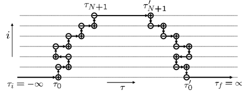
Figure 8: The electron world line representing the probability of elastic cotunneling from the $0-$th to the $N+1-$st grain.

IX.1 Hopping via elastic cotunneling

To analyze the hopping transport mechanism in granular array one has to consider the probability of electron tunnelling between the two distant grains with energies close to the Fermi level. At very low temperatures such a tunneling can be realized only as a virtual tunneling of an electron through several grains being in the Coulomb blockade regime - such a process is called the elastic cotunneling. Averin

In the following we consider the probability of elastic cotunnelling through several grains within the approach of effective classical model. We assume that the electron tunneling takes place between two sites $i_{0}$ and $i_{N+1}$ where the local Coulomb gap is absent. In our model it means that the Coulomb energy on these two sites is compensated by the external local potentials $\mu_{i}.$ Thus, removing the charge from the grain $i_{0}$ as well as placing it on the grain $i_{N+1}$ does not cost any Coulomb energy. The probability of tunnelling between these two states can be found as follows: In the basis of the eigenstates of a system of isolated grains the amplitude of tunnelling process from the site $i_{0}$ to the site $i_{N+1}$ is

$$A_{i_{0},i_{N+1}}=<0|\;\hat{c}_{i_{N+1}}\hat{S}\;\hat{c}^{\dagger}_{i_{0}}\,|0>,$$ (81)

where $\hat{S}$ is the evolution operator that written in the interaction representation takes into account only tunnelling part of the Hamiltonian (25a). Consideration of the amplitude $A_{i_{0},i_{N+1}}$, however, is not convenient since the amplitude becomes zero after averaging over tunnelling matrix elements $t_{k_{1},k_{2}}.$ This happens because the phase of the amplitude of tunnelling process is very sensitive to the particular realization of disorder. For this reason one has to consider the probability of the tunnelling process $P=A^{*}A.$ The conjugate amplitude $A^{*}$ can be written as the probability of the inverse process of tunnelling between $i_{N+1}-$st and $i_{0}-$th grains

$$A_{i_{0},i_{N+1}}^{*}=A_{i_{N+1},i_{0}}=<0|\;\hat{c}_{i_{0}}\,\hat{S}\;\hat{c}^{\dagger}_{i_{N+1}}\,|0>.$$ (82)

The probability of the tunnelling process $P=A^{*}A$ can be presented as an electron world-line shown in Fig. 8. The first interval of the world line ($\tau_{i},\tau_{0}$) represents the initial state of the system where the electron is located at the site $i_{0}.$ The following part ( $\tau_{0},\tau_{N+1}$ ) represents the amplitude of the tunnelling process $A_{i_{0},i_{N+1}}$ from the site $i_{0}$ to the site $i_{N+1}.$ The interval ($\tau_{N+1},\tau_{N+1}^{\prime}$) describes the system with the electron located on the site $i_{N+1}.$ The next interval ($\tau_{N+1}^{\prime},\tau_{0}^{\prime}$) represents the amplitude $A_{i_{N+1},i_{0}}$ of the process of tunnelling back to the site $i_{0},$ and the last interval ($\tau_{0}^{\prime},\tau_{f}$) represents the system back in the initial state where the electron is located at site $i_{0}.$

The world line that represents the tunnelling probability $P=A^{*}A$ is very similar to the closed loops in Fig. 7. The only difference is that in the world line of Fig. 8 the Green functions on the sites $i_{0}$ and $i_{N+1}$ must be taken in a different way: In order to capture the energy resolution of electron energies of the initial and final states we will assume that both sites $i_{0}$ and $i_{N+1}$ have only one quantum state each with energies $\xi_{0}$ and $\xi_{N+1}$ (counted with respect to the chemical potential) respectively.

When electron tunnels from site $i_{0}$ to site $i_{1},$ the hole is created at site $i_{0}.$ Such process is described by the Green function of a negative time argument Abrikos

$$G_{0}(\tau_{0}^{\prime}-\tau_{0})=n(\xi_{0})\;e^{\xi_{0}(\tau_{0}^{\prime}-\tau_{0})},$$ (83)

where $n(\xi)$ is the electron occupation number that reminds that the electron is assumed to be initially present at site $i_{0}$.

Similarly, the process when the electron is located on site $i_{N+1}$ is described by the Green function of positive arguments

$$G_{N+1}(\tau_{N+1}^{\prime}-\tau_{N+1})=[\,1-n(\xi_{N+1})\,]\;e^{-\xi_{N+1}(\tau_{N+1}^{\prime}-\tau_{N+1}),},$$ (84)

where the occupation number $1-n(\xi_{N+1})$ insures that the final state must be empty for an electron to be able to tunnel there.

Before proceeding to the calculation of tunneling probability let us first fix notations for all time coordinates in Fig. 8: To distinguish the time coordinates that belong to the left part of the world line representing the direct tunneling process from the ones that belong to the right part representing the inverse process we denote the later ones by primes. Further, to distinguish the time coordinates of positive and negative charges we use the index $+$ and $-$ respectively.

The tunneling probability $P$ represented by the world-line shown in Fig. 8 can be calculated easily for the case of a diagonal (short range) Coulomb potential $E^{\scriptscriptstyle C}_{ij}=\delta_{ij}E^{c}_{i}.$

IX.1.1 Short range Coulomb interaction

In this case time integrations on each site $k$ can be implemented independently and the tunneling probability $P$ is given by the product of probabilities $P_{k}$ representing the single site contributions. To find a single site contribution $P_{k}$ we note that there are two possible arrangements of the tunneling times: (i) $\tau_{k-}<\tau_{k+}<\tau_{k-}^{\prime}<\tau_{k+}^{\prime}$ and (ii) $\tau_{k+}<\tau_{k-}<\tau_{k+}^{\prime}<\tau_{k-}^{\prime}.$ Let us first consider the case (i): The Coulomb energy of such configuration is given by

$$U_{k}^{c(i)}=E_{k}^{+}\,(\Delta\tau_{k}+\Delta\tau_{k}^{\prime}),$$ (85)

where the electron excitation energy $E_{k}^{+}$ is given by Eq.(10) and the time intervals $\Delta\tau_{k},\Delta\tau_{k}^{\prime}>0$ are defined as $\Delta\tau_{k}=\tau_{k+}-\tau_{k-},\;\;\Delta\tau_{k}^{\prime}=\tau_{k+}^{\prime}-\tau_{k-}^{\prime}.$ The internal energy of the configuration according to Eq. (80) is

$${\cal U}_{k}=-\ln[g_{k}\delta/2\pi]+\ln(\Delta\tau_{k}+\Delta\tau_{k}^{\prime}),$$ (86)

where $g_{k}$ is the tunnelling conductance between the $k-$th and $(k+1)-$st grains. One can see that the second arrangement of charges (ii) differs only by the expression for the Coulomb energy

$$U_{k}^{c(ii)}=E^{-}_{k}\,(|\Delta\tau_{k}|+|\Delta\tau_{k}^{\prime}|).$$ (87)

Now with the help of Eqs. (85, 86, 87) we find the elementary probability $P_{k}$ determined by the sum of the contributions (i) and (ii) as

$$P_{k}={{g_{k}\delta}\over{2\pi}}\int_{0}^{\infty}d\Delta\tau\,d\Delta\tau^{\prime}\,{{e^{-E^{+}_{k}(\Delta\tau+\Delta\tau^{\prime})}+e^{-E^{-}_{k}(\Delta\tau+\Delta\tau^{\prime})}}\over{\Delta\tau+\Delta\tau^{\prime}}},$$

and taking the integrals we obtain

$$P_{k}={{g_{k}\,\delta}\over{\pi\tilde{E}_{k}}}.$$ (88)

where the energy $\tilde{E}_{k}$ is the combination of the energies $E^{+}_{k}$ and $E^{-}_{k}$ defined by Eq.(13).

To find the time dependence of the tunneling process we notice that the time intervals $\tau_{0}^{\prime}-\tau_{0}$ and $\tau_{N+1}^{\prime}-\tau_{N+1}$ coincide within the accuracy of the inverse charging energy. In the limit that we consider the charging energy is the largest scale in the problem that allows to take both intervals to be equal to the the ”width” of the loop $\tau_{w}$ that at the same time represents the time that electron spend on site $i_{N+1}.$ Thus, the time dependence of the tunneling process is simply given by

$$e^{-(\xi_{N+1}-\xi_{0})\tau_{w}}.$$ (89)

Making an analytical continuation to real times $\tau_{w}=it_{w}$ and taking the last integral over $t_{w}$ we obtain the delta function

$$2\pi\delta(\xi_{N+1}-\xi_{0}),$$ (90)

that indeed shows that the process is elastic, i.e. electron can tunnel only to the state with exactly the same energy.

Finally, for the tunneling probability of the elastic process we obtain

$$P_{el}=w\,\delta(\xi_{N+1}-\xi_{0})\,g_{0}\,\prod_{k=1}^{N}P_{k},$$ (91)

where the factor $w=n(\xi_{0})(1-n(\xi_{N+1})$ takes into account the occupation numbers of the initial and final states. We see that the total probability $P_{el}$ contains the product of all conductances, mean level spacings and inverse energies along the tunneling path. For this reason it is convenient to introduce the geometrical averages of theses quantities along the tunneling path that were introduced in Sec. II.2.1. Writing the total probability $P_{el}$ in terms of the quantities $\bar{g},\bar{\delta},\bar{E}$ we obtain the result (11).

IX.1.2 Long range Coulomb interaction

In the presence of the long range Coulomb interaction the situation is more complicated since the integrals over variables $\tau_{\pm k}$ cannot be taken on each site $k$ independently. However, one can estimate the tunnelling probability $P_{el}$ by finding its upper and lower limits: Indeed, neglecting the long range part of the potential (as we did above) one gets the upper boundary. The lower boundary can be obtained by considering such trajectories where all $\Delta\tau_{k}$ are of the same sign. In this case the electric field created by the charges on step $k$ does not interfere with other charges and thus one can implement integrations independently. This gives a lower boundary for the tunnelling probability $P_{k}$ which is about a factor 2 smaller than the tunnelling probability $P_{k}$ obtained neglecting the long range part of the Coulomb potential. This results in the boundaries of the factor $0.5\lesssim c<1.0$ in the expression for localization length $\xi_{el}$ in Eq. (14).

The above derivation of tunnelling probability $P_{el}$ has been done for the zero temperatures case. Of course the finite temperatures and the presence of phonons are necessary for the realization of the Mott-Efros-Shklovskii mechanism. Calculation of the tunneling probability at zero temperature is justified as long as inelastic tunneling processes that are considered in the next section can be neglected.

IX.2 Hopping via inelastic cotunneling

According to the theory of transport through a single quantum dot in the Coulomb blockade regime Averin , at temperatures $T>\sqrt{\delta E_{C}}$ the electron transport is dominated by inelastic cotunneling processes. In this case the process of charge transfer from one contact to the dot and the following process of charge transfer from the dot to the other contact is realized by means of different electrons. As a result, the energy of the outcoming electron differs from that of the incoming one and the dot energy is changed after the each elementary charge transfer process. For this reason inelastic cotunneling processes are allowed only either at finite temperature or if a finite voltage is applied to contacts.

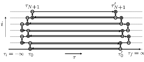
Figure 9: Tunneling via inelastic cotunneling between $0-$th to the $N+1-$st grains.

In order to include the inelastic cotunneling processes into the scheme that we described above, first, we have to generalize the charge representation to finite temperatures. The main difference is that the imaginary time $\tau$ at finite temperatures is constraint to the interval ($0,\beta),$ where $\beta=1/T$ is the inverse temperature. Also the expressions for internal energies must be properly modified. Using the Matsubara technique one can show that the proper expressions for the internal energies can be obtained from the corresponding expressions at zero temperature via the substitution $1/\tau\to\pi T/\sin(\pi T\tau),$ such that, for example, the quadruple internal energy given by Eq. (45) becomes

$${\cal U}_{n}^{q}=\ln[\,2\sin^{2}(\pi T|\Delta\tau|)/\,g\pi T^{2}\,].$$ (92)

In general, one should also take into account the static charges that formally appear from the integer winding numbers in the phase representation at finite temperature. However, inclusion of static charges is not needed for the description of virtual co-tunneling processes that we consider.

The representation of an inelastic cotunneling process in terms of the electron world lines is shown in Fig. 9. This process resembles the world line of the elastic co-tunneling process shown in Fig. 8 since the electron charge is transferred from the site $i_{0}$ to the site $i_{N+1}$ and then back to the site $i_{0}$ in essentially the same way. However, the important difference is that the diagram for the inelastic process is constructed out of quadruple loops only. This implies that the charge is transferred by means of deferent electrons on each hop.

As in the case of the elastic cotunneling we assume that the sites $i_{0}$ and $i_{N+1}$ have only one state each with energies $\xi_{0}$ and $\xi_{N+1}$ respectively. Similarly to the previous subsection consideration, we write down the Green functions representing the initial and final states: when electron tunnels from site $i_{0}$ to site $i_{1},$ a hole is created at site $i_{0}$. Such a process is described by the Green function of negative time arguments

$$G_{0}(\tau_{0}^{\prime}-\tau_{0})=n(\xi_{0})\;e^{\xi_{N+1}(\tau_{0}^{\prime}-\tau_{0})}.$$ (93)

The process where electron is located on the site $i_{N+1}$ is described by the Green function of positive arguments

$$G_{N+1}(\tau_{N+1}^{\prime}-\tau_{N+1})=[\,1-n(\xi_{N+1})\,]\;e^{-\xi_{N+1}(\tau_{N+1}^{\prime}-\tau_{N+1})}.$$ (94)

The time coordinates $\tau_{+k}$ and $\tau_{-k}$ are again confined within the temporal interval $\Delta\tau_{k}\sim 1/E^{c}_{0}$. This means that the time arguments of the quadruple energies ${\cal U}_{n}^{q}$ in Eq. (92) are approximately the same and equal to the “width” of the loop formed by the world line in Fig. 9: $\tau_{w}\approx\tau_{0}^{\prime}-\tau_{0}\approx\tau_{N+1}^{\prime}-\tau_{N+1}$. Thus, the contributions of quadruple internal energies ${\cal U}_{n}^{q}$ to the tunneling probability $P_{in}$ result in the factor

$$\left({{\bar{g}\pi T^{2}}\over{\sin^{2}(\pi T\tau_{w})}}\right)^{N},$$ (95)

where $\bar{g}$ is the geometrical average of the conductances over the electron path. Integrations over the intermediate times $\tau_{k}$ of the inelastic process can be easily done for the case of the diagonal Coulomb interaction $E_{ij}^{c}=E_{0}^{c}\delta_{ij}$.

IX.2.1 Short range Coulomb interaction

In the case of the short range interaction the integrations over $\Delta\tau_{k}$ and $\Delta\tau^{\prime}_{k}$ can be performed independently. Also the integrations over the $\Delta\tau_{k}$ and $\Delta\tau^{\prime}_{k}$ result in the equal contributions given by

$$\int_{-\infty}^{\infty}d\Delta\tau_{k}\;e^{-E_{k}^{c}|\Delta\tau_{k}|+\mu_{k}\Delta\tau_{k}}=2/\tilde{E}_{k},$$ (96)

where the energy $\tilde{E}_{k}$ is defined in Eq. (13). Collecting all the terms for the probability $P_{in}$ one obtains

$$P_{in}(\tau_{w})={{w\,\bar{g}^{N+1}}\over{2\pi^{N+1}}}\left({{2\pi T}\over{{\bar{E}}\sin(\pi T\tau_{w})}}\right)^{2N}e^{-\Delta\tau_{w}}.$$ (97)

Finally, in order to find the tunneling probability $P_{in}$ via the inelastic cotunneling one has to make the analytical continuation in Eq. (97) to the real times $\tau_{w}=it_{w}$ and integrate over $t_{w}$ arriving at

$$P_{in}={{w\,g^{N+1}}\over{2\pi^{N+1}}}\int\limits_{-\infty}^{+\infty}dt\left[{{2\pi iT}\over{{\bar{E}}\sinh(\pi Tt)}}\right]^{2N}e^{-i\Delta t}.$$ (98)

Here the singularity of the function $\sinh^{-2N}(\pi Tt)$ is taken in the upper half of the complex plain. At zero temperature one can easily calculate the integral over the variable $t$ in Eq. (98) by shifting the contour of integration in the complex plain either to negative complex infinity in the case of positive $\Delta$ or to the positive complex infinity in the case of negative $\Delta.$ In the first case we obtain $P_{in}=0$. This reflects the fact that the real tunneling process with increase of electron’s energy is forbidden at $T=0$. In the latter case, $\Delta<0$, the zero temperature probability is determined by the pole of the function $\sinh^{-2N}(\pi Tt)$ that results in the answer presented in Eq.(22).

At finite temperatures the integral in Eq. (98) can be expressed in terms of the the Euler Gamma functions that leads to the general expression (18).

IX.2.2 Long range Coulomb interaction

In the presence of the long range part of the Coulomb interaction the integrations over time variables on each step cannot be performed independently. This makes it difficult to derive an exact analytic formula for the tunneling probability. However, as in the case of the elastic cotunneling, one can easily estimate the upper and lower boundaries for this quantity: neglecting the off-diagonal part of the Coulomb interaction, as above, we get the upper boundary. The lower boundary can be obtained by considering the trajectories where all $\Delta\tau_{k}$ (as well as all $\Delta\tau_{k}^{\prime}$) have the same sign. This consideration constraints the values of the coefficient $c$ in the expression for the localization length to the interval $1/4\lesssim c<1$. One can also see that only the sites that are geometrically close to each other can interfere. Indeed, let us consider two sites $k_{1}$ and $k_{2}$ in the tunneling path that are relatively far from each other. Interference effects related to these sites can be included as a small correction. One can easily see that the first order correction vanishes because the average electric field on the site $k_{1}$ created by the charges on the site $k_{2}$ is zero and vias versa. Thus the contribution of the interference effects falls of with the distance as $1/r^{2}$ at least. These insures that there is no any dramatic effect related to the long-range part of the Coulomb interaction apart form the numerical correction in the localization length. The same arguments apply to the case of the elastic cotunneling.

X Mott transition in a periodic granular array

In this section we discuss the metal to insulator transition in the regular periodic granular arrays. The Mott gap $\Delta_{M}$ for such a system in the nearest neighbor hopping (quadruple) approximation considered in Sec. VII is exponentially small as function of conductance, Eq. (3), but always finite. In this section we consider how this result is affected by inclusion of high order tunneling processes that are represented by higher order loops in the classical model of Coulomb charges.

In Sec. IX it was shown that at $gz\ll 1$ the contribution of higher order tunnellings processes to the tunneling provability $P$ at zero temperature is suppressed by the factor

$$\left(\frac{g\,\delta}{E^{c}_{0}}\right)^{N},$$ (99)

where $N$ is the order of the tunneling process. It is clear that the same parameter defines the smallness of the contribution of the high order loops to the thermodynamic potential $\Omega$ of the classical gas. If the tunneling conductance is not small, $gz>1$, the Coulomb interaction of two classical charges is strongly renormalized and in this case instead of the bare Coulomb interaction $E_{0}^{c}$ in Eq. (99) one has to take the renormalized one - that is the Mott gap $\Delta_{M}$ given by Eq. (3). We come to the conclusion that the high order loops can be neglected as long as

$$\Delta_{M}>g\delta.$$ (100)

Equation (100) can be rewritten in terms of the intergranular tunneling conductance $g$ in the way

$$g<g_{c},$$ (101)

where the critical conductance $g_{c}$ is defined by Eq.(4). The samples characterized by the tunneling conductance $g<g_{c}$ at zero temperatures are insulators with the Mott gap $\Delta_{M}$ given by Eq. (3). The result (4) for the critical conductance $g_{c}$ coincides with the value of the stability of the metallic state obtained from the diagrammatic technique from the metallic side of the transition $g>g_{c}.$ BLV03 This fact confirms that the value (4) indeed separates the metallic and insulating states at $T=0.$

Note that the accuracy of the above considerations is not sufficient to establish whether the transition between the insulating and metallic states is continuous or discontinuous. The details of the behavior of the Mott gap $\Delta_{M}$ in the immediate vicinity of the critical conductance $g_{c}$ are not known yet.

So far we considered the limit of the zero temperature. Physics of the Mott transition at finite temperature depends crucially on whether the transition is continuous at $T=0$ or it is discontinuous. In the case of continues transition at $T=0$, at finite temperatures the metallic and insulating phases, strictly speaking, cannot be distinguished. Indeed, the Mott transition does not break any symmetry and the conductivity at finite temperatures is finite even in the ”insualting” phase where it acquires the activation form, Eq. (5). However, in the case of the first order phase transition at $T=0$, due to arguments of physical continuity, the transition has to remain of the first order in some interval of finite temperatures. Such transition would result in the jump of the physical observables even at finite temperatures.

XI Conclusions

We have investigated Coulomb interaction effects and transport properties of granular conductors in the insulating (dielectric) regime. We have considered both the periodic- and irregular arrays and took into account the random on-site electrostatic potential. We find the dependence of the Mott gap on the tunneling conductance in the dielectric regime of a regular array. The insulator to metal transition takes place at the critical conductance given by Eq.(4) where the Mott gap becomes of the order of the inverse escape time of the electron from a single grain $g\delta$. The order of the transition remains, however, an open question. For the case of irregular granular arrays we have derived the Efros-Shklovskii law for the conductivity of a granular system. Depending on the temperature the hopping conductivity is dominated by either elastic or inelastic cotunneling processes. In the latter case the localization length is weakly (logarithmically) depends on temperature. In particular, our model and the obtained results explain the origin of the ES conductivity in the spatially periodic arrays of semiconducting quantum dots.

Finally, we would like to discuss the possibility of the observation of the Mott law in granular metals. To remind, in semiconductors, the Efros-Shklovskii law may turn to the Mott behavior with the increase of temperature. This happens when the typical electron energy $\varepsilon$ involved in a hopping process becomes larger than the width of the Coulomb gap $\Delta_{c}$, i.e. when it falls into the flat region of the density of states where Mott behavior is expected. To estimate the width of the Coulomb gap $\Delta_{c}$ - one compares the ES expression (6) for the density of states with the bare density of states $\nu_{g_{0}}$, i.e. the DOS in the absences of the long-range part of the Coulomb interactions obtaining

$$\Delta_{c}=\left(\frac{\nu_{g_{0}}e^{2d}}{\tilde{\kappa}^{d}}\right)^{1\over{d-1}}.$$ (102)

As we discussed in Sec. II in granular metals the density of states $\nu_{g_{0}}$ that is relevant for hopping conductivity does not coincide with the physical DOS, since only the lowest energy excitations in a single grain must be counted in determination of $\nu_{g_{0}}.$ Shklovskii04

Bare density of ground sates $\nu_{g_{0}}$ can be easily estimated for the case of strong on-site disorder that we assumed so far as follows: The width of the potential distribution $\mu_{i}$ is approximately given by the average on-site Coulomb energy so that

$$\nu_{g_{0}}\approx 1/E^{c}_{0}\,a^{d}.$$ (103)

Inserting this value into Eq. (102) for the width of the Coulomb gap we obtain $\Delta_{c}\sim E^{c}_{0}$ meaning that there is no flat region in the density of ground states and, thus, the Mott regime is not possible. However, the Mott regime may appear in the case of weak electrostatic disorder ( for a detail discussion of this issue see Ref. Shklovskii04 ). In this case the subgap states will appear very rarely over the granular sample and the bare density of ground states $\nu_{g_{0}}$ is greatly reduced and as a result the width of the Coulomb gap substantially shrinks.

One can easily repeat all the considerations that led us to the expressions for the hopping conductivity for the case of flat density of ground states arriving to the Mott expression

$$\sigma\sim\sigma_{0}\;\exp[-(T_{0}^{M}/T)^{1\over{d+1}}],$$ (104)

where the temperature $T_{0}^{M}$ is given by

$$T_{0}^{M}\sim 1/\nu_{g_{0}}a^{d}\xi^{d},$$ (105)

with the dimensionless localization length $\xi$ given by either equation (14) or (21) depending on the temperature regime.

The crossover temperature $T^{*}$ between the two regimes is easily obtained exactly as in the case of semiconductors; by comparing Eqs. (1) and (104) and using the corresponding expressions for $T_{\circ}$ we get

$$T^{*}\sim e^{2}a\xi\left({{e^{4}\nu_{g_{0}}^{2}}\over{\tilde{\kappa}^{d+1}}}\right)^{1/(d-1)}.$$ (106)

As a final note, we would like to comment on the possibility of fixing the numerical coefficient in the expression for the temperature $T_{0}$ that enters exponents of the expressions for the hopping conductivity. In the case of hopping conductivity in semiconductors this coefficient can be fixed by means of the mapping the problem of the impurity states in semiconductors onto a simple classical percolation model that can be investigated completely numericallyAbrahams ; Halperin ; Shklovskii . In granular metals, on the qualitative level, the situation is very similar, however, it is not clear that a model of a granular metal can be reduced to a simple unique percolation problem without making additional uncontrolled assumptions. The main complications are that the tunneling process in granular metals (i) in general goes via the curved trajectory, (ii) it depends on the number of the parameters of the intermediate grains in the tunneling path as $E^{c}_{i},\delta_{i},g_{ij}.$ For this reason, in general, we expect that the coefficient in the expressions for $T_{0}$ is not universal and is dependent on the morphology of a granular sample.

After the present study was completed, we became aware of the preprint FI05 where the hopping transport in granular metals via elastic and inelastic cotunneling in the linear regime ( low applied voltage ) was considered; their results essentially agree with ours.

Appendix A Minimization of the probability of the inelastic cotunneling

The result for the hopping conductivity in the regime of inelastic cotunneling is obtained via minimization of expression (18) with respect to the hopping distance $N$ under constraint

$$Na\Delta\,\tilde{\kappa}\,/e^{2}=b,$$ (107)

following from the ES expression for the density of states, with $b$ being a constant. Minimization procedure can be easily implemented presenting the tunneling probability $P_{in}$ as

$$P_{in}\sim e^{A},$$ (108)

with the action $A$ given by

$$A = -{{2N}\over\xi_{in}}+\ln\Gamma(N+i\Delta/2\pi T)$$ (109)

$$+ \ln\Gamma(N-i\Delta/2\pi T)-\ln\Gamma(2N)-\Delta/2T,$$

where $\xi_{in}$ is the localization length given by (21). Taking into account that according to Eq.(107) $d\Delta/dN=-\Delta/N$ minimization of the action $A$ with respect to $N$ in the limit of the large $N$ results in the equation

$$\ln 4+2/\xi_{in}=\ln(1+x^{2})+\pi x\,[1+(2/\pi)\arctan x],$$ (110)

where the parameter $x$ is defined as

$$x=\Delta/2\pi TN.$$ (111)

We see that Eq.(110) fixes the ratio $\Delta/TN$ for a given localization length. Using Eq.(110) and that $N\gg 1$ the action (109) can be simplified to

$$A=-{\Delta\over{T}}\left(1+{2\over\pi}\arctan x\right),$$ (112)

that with the help of Eqs.(107,111) can be further written in terms the parameter $x$ as

$$A=-\sqrt{{2\,b\,e^{2}}\over{aT\tilde{\kappa}}}\,\sqrt{x\pi}\;[1+(2/\pi)\arctan x].$$ (113)

Within the logarithmic accuracy we can consider the localization length as a small parameter. In this case Eq.(110) gives that $x\approx 1/\pi\xi$ and from the above equation we finally obtain the resulting action

$$A\approx-\sqrt{{{8\,b\,e^{2}}\over{\xi_{in}a\,T\tilde{\kappa}}}}.$$ (114)

We would like to note that, in principle, one should consider an alternative minimization scheme for the tunneling process: The tunneling first occurs with $\Delta=0$ as in the case of the elastic process, and then the electron gets an extra energy due to phonon or electron collision not included directly in the probability of the inelastic process under consideration. One can easily show that in this case one would get $A=-\sqrt{8\,b\,e^{2}\,/T\,a\,\xi_{in}\tilde{\kappa}}$ that coincides with the action (114) obtained in the leading order in the parameter $1/\xi_{in}.$ One can check, however, that taking large but finite $1/\xi_{in}$ results in a correction to the action (114) that consist of the reduction of the coefficient $\sqrt{8}.$ Thus the process with intrinsic inelasticity that we considered is a bit more favorable. This insures that the minimization scheme used by us is the right one.

References

- (1) A. Gerber, A. Milner, G. Deutscher, M. Karpovsky, and A. Gladkikh, Phys. Rev. Lett. 78, 4277 (1997).
- (2) R. Parthasarathy, Xiao-Min Lin, K. Elteto, T. F. Rosenbaum, and H. M. Jaeger, Phys. Rev. Lett. 92, 076801 (2004).
- (3) K. B. Efetov and A. Tschersich, Europhys. Lett. 59, 114, (2002); Phys. Rev. B 67, 174205 (2003).
- (4) J. Zhang and B. I. Shklovskii, Phys. Rev. B 70, 115317 (2004).
- (5) I. S. Beloborodov, K. B. Efetov, A. V. Lopatin and V. M. Vinokur, Phys. Rev. Lett 91, 246801 (2003).
- (6) I. S. Beloborodov, A. V. Lopatin, and V. M. Vinokur Phys. Rev. B 70, 205120 (2004).
- (7) M. V. Feigel’man, A. S. Ioselevich, and M. A. Skvortsov, Phys. Rev. Lett 93, 136403 (2004).
- (8) V.I.Kozub, V.M.Kozhevin, D.A.Yavsin, S.A.Gurevich, Pis’ma v ZhETP, v.80, N5, (2005).
- (9) Y. L. Loh, V. Tripathi, M. Turlakov, cond-mat/0501749.
- (10) B. L. Altshuler and A. G. Aronov, in Electron-Electron Interaction in Disordered Systems, ed. by A. L. Efros and M. Pollak, North-Holland, Amsterdam (1985).
- (11) L. P. Gorkov, A. L. Larkin and D. E. Khmel nitskii, Pis ma Zh. Eksp. Teor. Fiz. 30, 248 (1979) [Sov. Phys. JETP Lett. 30, 228 (1979)].
- (12) P. Sheng, B. Abeles, and Y. Arie, Phys. Rev. Lett. 31, 44 (1973); B. Abeles, P. Sheng, M. D. Coutts, and Y. Arie, Adv. Phys. 24, 407 (1975).
- (13) M. Pollak and C. J. Adkins, Phil. Mag. B 65, 855 (1992).
- (14) L. Efros and B. I. Shklovskii, J. Phys. C 8, L49 (1975)
- (15) I. S. Beloborodov, A. V. Lopatin, V. M. Vinokur, and V. I. Kozub, cond-mat/0501094.
- (16) V. Ambegaokar, U. Eckern, and G. Schön, Phys. Rev. Lett. 48, 1745 (1982); for review see Ref.[Zaikin, ].
- (17) A. Schmid, Phys. Rev. Lett. 51, 1506 (1983).
- (18) A. Georges, G. Kotliar, W. Krauth, and M. J. Rozenberg Rev. Mod. Phys. 68, 13-125 (1996).
- (19) A.I. Yakimov, A.V. Dvurechenskii, G.M. Min’kov, A.A Sherstobitov, A.I. Nikiforov and A.A. Bloshkin, to be published in JETP.
- (20) T. Tran, Xiao-Min Lin and H. Jaeger, to be published.
- (21) B. I. Shklovskii and A. L. Efros, Electronic properties of Doped Semiconductors, Springer-Verlag, New York, 1988).
- (22) We consider the system periodic if (i) all the granules are of the same size and shape and arranged in a regular structure; (ii) all the tunneling conductances between the nearest neighbors are equal; and (iii) there is no disorder in the dielectric matrix that causes local fluctuations in granules’ chemical potential.
- (23) M. Muller and L.B. Ioffe, Phys. Rev. Lett. 93, 256403 (2004)
- (24) S. Pankov and V. Dobrosavlijevic, Phys. Rev. Lett. 94 046402 (2005).
- (25) Eq. (18) gives the probaillity of spin unresolved process, i.e. it includes the sum over spin components of the final state.
- (26) N. F. Mott, Adv. Phys. 16, 49 (1967).
- (27) G. Schön and A.D. Zaikin, Phys. Rep. 198, 237 (1990).
- (28) D. A. Averin and Yu. V. Nazarov, Phys. Rev. Lett. 65, 2446 (1990).
- (29) J. E. Mooij, B. J. van Wees, L. J. Geerligs, M. Peters, R. Fazio, and G. Schön, Phys. Rev. Lett. 65, 645 648 (1990).
- (30) J. S. Meyer, A. Kamenev, and L. I. Glazman, Phys. Rev. B 70, 045310 (2004).
- (31) A. Altland, L. I. Glazman, and A. Kamenev, Phys. Rev. Lett. 92, 026801 (2004).
- (32) B. I Shklovskii, Fiz. Tekh. Poluprovodn. (S.-Petersburg) 6, 2335 (1973) [Sov. Phys. Semicond. 6,1964 (1973)].
- (33) L. D. Landau and I. M. Lifshitz, Quantum mechnics, 3d ed., Elsevier Science, Oxford (1977).
- (34) We use the dimensionless units for energy of the classical model assuming that the effective temperature
- (35) D. P. Arovas, F. Guinea, C. P. Herrero, and P. San Jos , Phys. Rev. B 68, 085306 (2003).
- (36) I. S. Beloborodov, K. B. Efetov, A. Altland and F. W. J. Hekking, Phys. Rev. B 63, 115109 (2001).
- (37) A.A. Abrikosov, L.P. Gor’kov, I.E. Dzyaloshinski, Methods of quantum field theory in statistical physics, Dover Publications, Inc. New York.
- (38) V.Ambegokar, B.I.Halperin, and J.S.Langer, Phys.Rev.B 4, 2612 (1971).
- (39) A. Miller and E. Abrahams, Phys. Rev. 120, 745 (1960).
- (40) M. V. Feigel’man, A. S. Ioselevich, cond-mat/0502481.