Quantum Spin Hall Effect
Abstract
The quantum Hall liquid is a novel state of matter with profound emergent properties such as fractional charge and statistics. Existence of the quantum Hall effect requires breaking of the time reversal symmetry caused by an external magnetic field. In this work, we predict a quantized spin Hall effect in the absence of any magnetic field, where the intrinsic spin Hall conductance is quantized in units of . The degenerate quantum Landau levels are created by the spin-orbit coupling in conventional semiconductors in the presence of a strain gradient. This new state of matter has many profound correlated properties described by a topological field theory.
Recently, the intrinsic spin Hall effect has been theoretically predicted for semiconductors with spin-orbit coupled band structuresMurakami et al. (2003); J. Sinova et. al. (2004). The spin Hall current is induced by the external electric field according to the equation
| (1) |
where is the spin current of the -th component of the spin along the direction , is the electric field and is the totally antisymmetric tensor in three dimensions. The spin Hall effect has recently been detected in two different experimentsY. Kato et. al. ; J. Wunderlich et.al. , and there is strong indication that at least one of them is in the intrinsic regimeBernevig and Zhang (a). Because both the electric field and the spin current are even under time reversal, the spin current could be dissipationless, and the value of could be independent of the scattering rates. This is in sharp contrast with the extrinsic spin Hall effect, where the effect arises only from the Mott scattering from the impurity atomsMott (1929).
The independence of the intrinsic spin Hall conductance on the impurity scattering rate naturally raises the question whether it can be quantized under certain conditions, similar to the quantized charge Hall effect. We start off our analysis with a question: Can we have Landau Level (LL) -like behavior in the absence of a magnetic field hal ? The quantum Landau levels arise physically from a velocity dependent force, namely the Lorentz force, which contributes a term proportional to in the Hamiltonian. Here is the particle momentum and is the vector potential, which in the symmetric gauge is given by . In this case, the velocity dependent term in the Hamiltonian is proportional to .
In condensed matter systems, the only other ubiquitous velocity dependent force besides the Lorentz force is the spin-orbit coupling force, which contributes a term proportional to in the Hamiltonian. Here is the electric field, and is the Pauli spin matrix. Unlike the magnetic field, the presence of an electric field does not break the time reversal symmetry. If we consider the particle momentum confined in a two dimensional geometry, say the plane, and the electric field direction confined in the plane as well, only the component of the spin enters the Hamiltonian. Furthermore, if the electric field is not constant but is proportional to the radial coordinate , as it would be, for example, in the interior of a uniformly charged cylinder , then the spin-orbit coupling term in the Hamiltonian takes the form . We see that this system behaves in such a way as if particles with opposite spins experience the opposite “effective” orbital magnetic fields, and a Landau level structure should appear for each spin orientations.
However, such an electric field configuration is not easy to realize. Fortunately, the scenario previously described is realizable in zinc-blende semiconductors such as GaAs, where the shear strain gradients can play a similar role. Zinc-blende semiconductors have the point-group symmetry which is half of the cubic-symmetry group , and does not contain inversion as one of its symmetries. Under the point group, the cubic harmonics transform like the identity, and off-diagonal symmetric tensors (, etc.) transform in the same way as vectors on the other direction (, etc), and represent basis functions for the representation of the group. Specifically, strain is a symmetric tensor , and its off-diagonal (shear) components are, for the purpose of writing down a spin-orbit coupling Hamiltonian, equivalent to an electric field in the remaining direction:
| (2) |
The Hamiltonian for the conduction band of bulk zinc-blende semiconductors under strain is hence the analogous to the spin-orbit coupling term . In addition, we have the usual kinetic term and a trace of the strain term , both of which transform as the identity under :
| (3) |
For GaAs, the constant M. I. Dyakonov et. al. (1986). This Hamiltonian is not new and was previously written down in Ref. J.E.Pikus and Titkov ; W.Howlett and Zukotynski (1977); Khaetskii and Nazarov (2001); T.B.Bahder (1990) but the analogy with the electric field and its derivation from a Lorentz force is suggestive enough to warrant repetition. There is yet another term allowed by group theory in the Hamiltonian Bernevig and Zhang (b), but this is higher order in perturbation theory and hence not of primary importance.
Let us now presume a strain configuration in which but has a constant gradient along the direction while has a constant gradient along the direction. This case then mimics the situation of the electric field inside a uniformly charged cylinder discussed above, as and , being the magnitude of the strain gradient. With this strain configuration and in a symmetric quantum well in the plane, which we approximate as being parabolic, the above Hamiltonian becomes:
| (4) |
We first solve this Hamiltonian and come back to the experimental realization of the strain architecture in the later stages of the paper. We make the coordinate change , and . or is a special point, where the Hamiltonian can be written as a complete square, namely with . At this point, our Hamiltonian is exactly equivalent to the usual Hamiltonian of a charged particle in an uniform magnetic field, where the two different spin directions experience the opposite directions of the “effective” magnetic field. Any generic confining potential can be written as , where the first term completes the square for the Hamiltonian, and the second term describes the additional static potential within the Landau levels. Since we can use the spin on the direction to characterize the states. In the new coordinates, the Hamiltonian takes the form:
| (7) | |||
| (8) |
The is the Hamiltonian for the down and up spin respectively. Working in complex-coordinate formalism and choosing we obtain two sets of raising and lowering operators:
| (9) |
in terms of which the Hamiltonian decouples:
| (10) |
The eigenstates of this system are harmonic oscillators of energy . We shall focus on the case of where there is no additional static potential within the Landau level.
For the spin up electron, the vicinity of is characterized by the Hamiltonian with the LLL wave function . is the operator moving between different Landau levels, while is the operator moving between different degenerate angular momentum states within the same LL: , . The wave function, besides the confining factor, is holomorphic in , as expected. These up spin electrons are the chiral, and their charge conductance is quantized in units of .
For the spin down electron, the situation is exactly the opposite. The vicinity of is characterized by the Hamiltonian with the LLL wave function . is the operator moving between different Landau levels, while is the operator between different degenerate angular momentum states within the same LL: , . The wave function, besides the confining factor, is anti-holomorphic in . These down spin electrons are anti-chiral, and their charge conductance is quantized in units of .
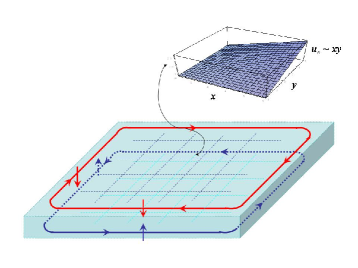
The picture that now emerges is the following: our system is equivalent to a bilayer system; in one of the layers we have spin down electrons in the presence of a down-magnetic field whereas in the other layer we have spin up electrons in the presence of an up-magnetic field. These two layers are placed together. The spin up electrons have positive charge Hall conductance while the spin down electrons have negative charge Hall conductance. As such, the charge Hall conductance of the whole system vanishes. The time reversal symmetry reverses the directions of the “effective” orbital magnetic fields, but interchanges the layers at the same time. However, the spin Hall conductance remains finite, as the chiral states are spin-up while the anti-chiral states are spin-down, as shown in Figure[1]. The spin Hall conductance is hence quantized in units of . Since an electron with charge also carries spin , a factor of is used to convert charge conductance into the spin conductance.
While it is hard to experimentally measure the spin Hall effect, and supposedly even harder to measure the quantum version of it, the measurement of the charge quantum Hall effect has become relatively common. In our system, however, the charge Hall conductance vanishes by symmetry. However, we can use our physical analogy of the two layer system placed together. In each of the layers we have a charge Quantum Hall effect at the same time (since the filling is equal in both layers), but with opposite Hall conductance. However, when on the plateau, the longitudinal conductance also vanishes () separately for the spin-up and spin-down electrons, and hence vanishes for the whole system. Of course, between plateaus it will have non-zero spikes (narrow regions). This is the easiest detectable feature of the new state, as the measurement is entirely electric. Other experiments on the new state could involve the injection of spin-polarized edge states, which would acquire different chirality depending on the initial spin direction.
We now discuss the realization of a strain gradient of the specific form proposed in this paper. The strain tensor is related to the displacement of lattice atoms from their equilibrium position in the familiar way . Our strain configuration is as well as the strain gradients and . Having the diagonal strain components non-zero will not change the physics as they add only a chemical potential term to the Hamiltonian. The above strain configuration corresponds to a displacement of atoms from their equilibrium positions of the form . This can be possibly realized by pulverizing GaAs on a substrate in MBE at a rate which is a function of the position of the pulverizing beam on the substrate. The GaAs pulverization rate should vary as , where is the distance from one of the corners of the sample where the GaAs depositing was started. Conversely, we can keep the pulverizing beam fixed at some and rotate the sample with an angle-dependent angular velocity of the form . We then move to the next incremental distance , increase the beam rate as and again start rotating the substrate as the depositing procedure is underway.
The strain architecture we have proposed to realize the Quantum Spin Hall effect is by no means unique. In the present case, we have re-created the so-called symmetric gauge in magnetic-field language, but, with different strain architectures, one can create the Landau gauge Hamiltonian and indeed many other gauges. The Landau gauge Hamiltonian is maybe the easiest to realize in an experimental situation, by growing the quantum well in the direction. This situation creates an off-diagonal strain , and where is the lattice mismatch (or impurity concentration), is a material constant and are the cubic axes. The spin-orbit part of the Hamiltonian is now . However, since the growth direction of the well is we must make a coordinate transformation to the coordinates of the quantum well ( are the new coordinates in the plane of the well, whereas is the growth coordinate, perpendicular to the well and identical to the direction in cubic axes). The coordinate transformation reads: , , , and the momentum along is quantized. We now vary the impurity concentration (or vary the speed at which we deposit the layers) linearly on the direction of the quantum well so that where is strain gradient, linearly proportional to the gradient in . In the new coordinates and for this strain geometry, the Hamiltonian reads:
| (11) |
where we have added a confining potential. At the suitable match between and , this is the Landau-gauge Hamiltonian. One can also replace the soft-wall condition (the Harmonic potential) by hard-wall boundary condition.
We now estimate the Landau Level gap and the strain gradient needed for such an effect, as well as the strength of the confining potential. In the case the energy difference between Landau levels is . For a gap of , we hence need a strain gradient or over . Such a strain gradient is easily realizable experimentally, but one would probably want to increase the gap to or more, for which a strain gradient of over or larger is desirable. Such strain gradients have been realized experimentally, however, not exactly in the configuration proposed here Q. Shen et. al. (1996); Shen and Kycia (1997). The strength of the confining potential is in this case which corresponds roughly to an electric field of for a sample of . In systems with higher spin-orbit coupling, would be larger, and the strain gradient field would create a larger gap between the Landau levels.
We now turn to the question of the many-body wave function in the presence of interactions. For our system this is very suggestive, as the wave function incorporates both holomorphic and anti-holomorphic coordinates, by contrast to the pure holomorphic Laughlin states. Let the up-spin coordinates be while the down-spin coordinates be the . enter in holomorphic form in the wave function whereas enter anti-holomorphically. While if the spin-up and spin-down electrons would lie in separate bi-layers the many-body wave function would be just , where is an odd integer. Since the particles in our state reside in the same quantum well and may possibly experience the additional interaction between the different spin states, a more appropriate wave function is:
| (12) |
The above wave function is symmetric upon the interchange reflecting the spin- chiral - spin- anti-chiral symmetry. This wave function is of course analogous to the Halperin’s wave function of two different spin states Halperin (1983). The key difference is that the two different spin states here experience the opposite directions of magnetic fields.
Many profound topological properties of the quantum Hall effect are captured by the Chern-Simons-Landau-Ginzburg theoryZhang et al. (1989). While the usual spin orbit coupling for spin- systems is -invariant but -breaking, our spin-orbit coupling is also -invariant due to the strain gradient. The low energy field theory of the spin Hall liquid is hence a double Chern-Simons theory with the action:
| (13) |
where the and fields are associated with the left and right movers of our theory while is the filling factor. The fractional charge and statistics of the quasi-particle follow easily from this Chern-Simons action. Essentially, the two Chern-Simons terms have the same filling factor and hence the Hilbert space is not the tensor product of any two algebras, but of two identical ones. This is a mathematical statement of the fact that one can insert an up or down electron in the system with the same probability. Such special theories avoids the chiral anomaly M. Freedman et. al. and their Berry phases have been recently proposed as preliminary examples of topological quantum computation M. Freedman et. al. . It is refreshing to see that such abstract mathematical models can be realized in conventional semiconductors.
A similar situation of Landau levels without magnetic field arises in rotating BECs where the mean field Hamiltonian is similar to either or . In the limit of rapid rotation, the condensate expands and becomes effectively two-dimensional. The term is induced by the rotation vector Ho (2001). The LLL behavior is achieved when the rotation frequency reaches a specific value analogous to the case in our Hamiltonian. In the BEC literature this is the so called mean-field quantum Hall limit and the ground state wave function is Laughlin-type. In contrast to our case, the theory is still breaking, the magnetic field is replaced by a rotation axial vector, and the lowest Landau level is chiral.
In conclusion we predict a new state of matter where a quantum spin Hall liquid is formed in conventional semiconductors with spin-orbit coupling. The quantum Landau levels are caused by the gradient of strain field, rather than the magnetic field. The new quantum spin Hall liquid state shares many emergent properties similar to the charge quantum Hall effect, however, unlike the charge quantum Hall effect, our system does not violate time reversal symmetry.
We wish to thank S. Kivelson, E. Fradkin, J. Zaanen, D. Santiago and C. Wu for useful discussions. B.A.B. acknowledges support from the Stanford Graduate Fellowship Program. This work is supported by the NSF under grant numbers DMR-0342832 and the US Department of Energy, Office of Basic Energy Sciences under contract DE-AC03-76SF00515.
References
- Murakami et al. (2003) S. Murakami, N. Nagaosa, and S. Zhang, Science 301, 1348 (2003).
- J. Sinova et. al. (2004) J. Sinova et. al., Phys. Rev. Lett. 92, 126603 (2004).
- (3) Y. Kato et. al., Science, 11 Nov 2004 (10.1126/science.1105514).
- (4) J. Wunderlich et.al., cond-mat/0410295.
- Bernevig and Zhang (a) B. Bernevig and S. Zhang, cond-mat/0411457.
- Mott (1929) N. Mott, Proc. Roy. Soc. 124, 425 (1929).
- (7) A related question was posed by F.D.M. Haldane (Phys. Rev. Lett. 61, 2015 (1988)) on whether the Quantum Hall effect necessarily requires an external magnetic field or can arise as a consequence of magnetic ordering in two-dimensional systems. The state proposed breaks time-reversal due to a local magnetic flux density of zero total flux through the unit cell.
- M. I. Dyakonov et. al. (1986) M. I. Dyakonov et. al., Sov. Phys. JETP 63, 655 (1986).
- (9) J.E.Pikus and A. Titkov, Optical Orientation (North Holland, Amsterdam, 1984, p. 73).
- W.Howlett and Zukotynski (1977) W.Howlett and S. Zukotynski, Phys. Rev. B 16, 3688 (1977).
- Khaetskii and Nazarov (2001) A. Khaetskii and Y. Nazarov, Phys. Rev. B 64, 125316 (2001).
- T.B.Bahder (1990) T.B.Bahder, Phys. Rev. B 41, 11992 (1990).
- Bernevig and Zhang (b) B. Bernevig and S. Zhang, cond-mat/0408442, accepted in Phys. Rev. B.
- Q. Shen et. al. (1996) Q. Shen et. al., Phys. Rev. B 54, 16381 (1996).
- Shen and Kycia (1997) Q. Shen and S. Kycia, Phys. Rev. B 55, 15791 (1997).
- Halperin (1983) B. Halperin, Helv. Phys. Acta 56, 75 (1983).
- Zhang et al. (1989) S. C. Zhang, H. Hansson, and S. Kivelson, Phys. Rev. Lett. 62, 82 (1989).
- (18) M. Freedman et. al., cond-mat/0307511.
- Ho (2001) T. Ho, Phys. Rev. Lett. 87, 060403 (2001).