Extinction of BKT transition by nonmagnetic disorder in planar-symmetry spin models

Abstract

The Berezinskii-Kosterlitz-Thouless (BKT) transition in two-dimensional planar rotator and XY models on a square lattice, diluted by randomly placed vacancies, is studied here using hybrid Monte Carlo simulations that combine single spin flip, cluster and over-relaxation techniques. The transition temperature $T_{c}$ is determined as a function of vacancy density $\rho_{\textrm{vac}}$ by calculations of the helicity modulus and the by finite-size scaling of the in-plane magnetic susceptibility. The results for $T_{c}$ are consistent with those from the much less precise fourth-order cumulant of Binder. $T_{c}$ is found to decrease monotonically with increasing $\rho_{\textrm{vac}}$, and falls to zero close to the square lattice percolation limit, $\rho_{\textrm{vac}}\approx 0.41$ . The result is physically reasonable: the long-range orientational order of the low-temperature phase cannot be maintained in the absence of sufficient spin interactions across the lattice.

I Introduction: Spin-Diluted Planar Spin Models

It is well known that vortices are fundamental ingredients in the Berezinskii-Kosterlitz-Thouless (BKT) phase transition. Berezinskii70 ; Berezinskii72 ; Kosterlitz73 The simplest models exhibiting this transition are the pure planar rotator model (PRM) and XY-model. For these models the transition takes place at critical temperatures $k_{B}T_{KT}/JS^{2}=0.898$ Tobochnik79 and $k_{B}T_{KT}/JS^{2}=0.699$, Cuccoli+95 ; Evertz96 respectively ($J$ is the exchange constant, $S$ the spin length). Recently, the study of topological excitations such as vortices and solitons in two-dimensional magnetic lattices containing defects has received a lot of attention. Subbaraman+98 ; Zaspel+96 ; Bogdan02 ; Pereira03 ; Pereira+03 ; Wysin03 ; Paula+04 ; Pereira+05 ; Karatsuji96 Such interactions must have interesting consequences for the static and dynamical properties of easy-plane magnets. Analytical and numerical calculations have shown that vortices are attracted and pinned by nonmagnetic impurities. Pereira03 ; Pereira+03 ; Paula+04 ; Mol+03 In fact, the vortex energy is lowered when pinned at a vacancy, resulting in greater preference of single vortex Wysin03 and vortex-pair Pereira04 formation on vacancies. Of course, this leads to an overall increase of the system disorder. All of these factors conspire to reduce the BKT transition temperature with increasing vacancy density, as has already been seen in calculations from Refs. Leonel+03, ; Berche+03, ; Wysin05, for planar spin models on a two-dimensional square lattice (see also analytical results using the self-consistent harmonic approximation of Ref. Castro+02, ). The important question here is, at what vacancy density is the transition temperature reduced to zero, so that the system is always in the high-T disordered phase? This would mean a situation in which there is no low-temperature phase of long-range orientational order, characterized by spin-spin correlations decaying as a power law with distance, and a finite absolute magnetization $\langle|\sum_{i}\vec{S}_{i}|\rangle$ in the thermodynamic limit.

Calculations of the helicity modulus for the planar rotator model by Leonel et al.Leonel+03 indicated that a critical vacancy density $\rho_{\textrm{vac}}=\rho_{c}\approx 0.3$ causes the critical temperature $T_{c}$ to drop to zero. It means that the critical temperature would vanish at $p_{c}=1-\rho_{c}\approx 0.7$, which is above the site percolation threshold, $p_{pt}=1-\rho_{pt}=0.59$, for a planar square lattice. Lozovick and Pomirchi, Lozovik93 also using the jump in the helicity modulus, have found that the BKT phase transition occurs above the percolation threshold in a dilute system of Josephson junctions (using bond dilution). On the other hand, Berche et al.Berche+03 calculated the decay of the spin-spin correlation function and its related exponent, $\eta$, and considered the transition temperature to be located by $\eta(T_{c})=1/4$. Those results suggested that the critical density is closer to $0.41$ (the number associated with the percolation limit for the square lattice). The Monte Carlo calculations for this problem naturally are particularly difficult, especially because the interesting region occurs at very low temperature. Furthermore, the statistical fluctuations due to the random choice of positions for the vacancies further increases the numerical noise in the calculations – this effect itself becomes particularly troublesome especially when $\rho_{\textrm{vac}}$ surpasses 0.3 (30%). As such, it seems important to make more reliable estimates for the critical vacancy density based on improved MC calculations here.

The calculations mentioned above concern the planar rotator model (two-component spins lying in xy plane). In a specialized model with repulsive vacancies, Wysin calculated the reduction of $T_{c}$ in an easy-plane Heisenberg model, with three-component spins with anisotropic couplings of their components.Wysin05 The vacancies were not allowed to be on nearest or next nearest neighbor lattice sites, which made it possible to calculate the vorticity density in the model. However, that calculation did not concern itself with the determination of the critical vacancy density, because the constraint of repulsive vacancies limits the possible vacancy density to be less than 18%, well below the critical value. Therefore, for comparison with the planar rotator, we also consider here the vacancy effects in the (three-component) XY-model, with randomly placed non-repulsive vacancies.

After describing the model Hamiltonians, we give an overview of the different methods used to estimate the transition temperature. This is followed by some specific comments on the Monte Carlo schemes applied to this problem. The data obtained for the planar rotator and XY models are presented, followed ultimately by our conclusions.

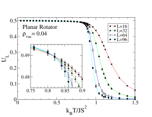
Figure 1: Application of the fourth order cumulant (5) for estimating $T_{c}$, for the PRM at 4% vacancy concentration. The data were obtained using the Monte Carlo approach described in Sec. II.2. The inset expands the view near the critical temperature ($k_{B}T_{c}/JS^{2}\approx 0.815$).

II Model Hamiltonians

The spin models under consideration can be described by the Hamiltonian

$$H=-J\sum_{\langle i,j\rangle}\sigma_{i}\sigma_{j}\left(S_{i}^{x}S_{j}^{x}+S_{i}^{y}S_{j}^{y}\right),$$ (1)

where $\langle i,j\rangle$ indicates nearest neighbor sites of an $L\times L$ square lattice, and $J$ is the ferromagnetic exchange coupling between spins $\vec{S}_{i}$ and $\vec{S}_{j}$. The spins $\vec{S}_{i}$ have two components for the planar rotator model and three components for the XY-model; in the latter case, however, only the xy components are coupled. The occupation variables $\sigma$ take the values $1$ or $0$ depending on whether the associated site is occupied by a spin or vacant. A fraction $\rho_{\textrm{vac}}$ of the sites are chosen randomly to be vacant. It is important to realize, however, that the Monte Carlo calculations here must make adequate averages over different choices of the vacancy positions, for a chosen density.

The planar rotator model has effectively a single degree of freedom per site – the angle of the spin within the xy plane. The main distinction of the XY model is the presence of the extra $S^{z}$ components, which act as degrees of freedom, but do not appear in the Hamiltonian. The XY model therefore involves two degrees of freedom per spin. This increases the entropy effects at a given temperature and results in a lower $T_{c}$ compared to the planar rotator. The MC algorithm for the XY model must involve the possibility to change all three spin components for the XY model, while preserving the spin length.

II.1 Physical properties leading to $T_{c}$

The lack of significant sharp peaks in the thermodynamic quantities versus temperature $T$ for these models, especially in finite $L\times L$ lattice systems, means that precisely locating $T_{c}$ is difficult. Therefore, it is useful to apply several different approaches, all essentially based on the scaling of the thermodynamics with the system size or edge length $L$.

As the Monte Carlo algorithm proceeds, the total system instantaneous in-plane magnetization $\vec{M}=(M_{x},M_{y})$ is observed,

$$\vec{M}=\sum_{i}\sigma_{i}\vec{S}_{i}.$$ (2)

Additionally, statistical fluctuations give the susceptibility components for temperature $T$,

$$\chi^{\alpha\alpha}=(\langle M_{\alpha}^{2}\rangle-\langle M_{\alpha}\rangle^{2})/(NT).$$ (3)

The number of spins in the system is $N=(1-\rho_{\textrm{vac}})L^{2}$. The average of $\chi^{xx}$ and $\chi^{yy}$ defines the in-plane susceptibility,

$$\chi=\frac{1}{2}(\chi^{xx}+\chi^{yy}).$$ (4)

A rough estimate of $T_{c}$ can be obtained from the size-dependence of Binder’s fourth order cumulantBinder81 ; Binder90 $U_{L}$, defined by

$$U_{L}=1-\frac{\langle(M_{x}^{2}+M_{y}^{2})^{2}\rangle}{2\langle M_{x}^{2}+M_{y}^{2}\rangle^{2}}.$$ (5)

For any $L$, the asymptotic values are $U_{L}(T\ll T_{c})=0.5$, $U_{L}(T\gg T_{c})=0$. At the critical temperature, $U_{L}$ is approximately independent of the system size, hence, $T_{c}$ can be estimated from the crossing point of curves of $U_{L}(T)$ for various $L$. An example of such crossing behavior is given in Fig. 1, for the PRM at $\rho_{\textrm{vac}}=0.04$. In practical application, due to the statistical uncertainties, there is usually no clear crossing point, especially at higher vacancy concentrations. Instead, $T_{c}$ is very close to the point where different curves of $U_{L}(T)$ begin to separate from the low-T asymptotic value. Although very reliable, this approach is not very accurate, and requires MC calculations for many temperatures near $T_{c}$.

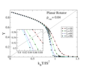
Figure 2: Typical application of the helicity modulus for estimating $T_{c}$, for the PRM at 4% vacancy concentration. The dashed line is Eq. (9). The inset shows how the crossing points occur slightly above the critical temperature ($k_{B}T_{c}/JS^{2}\approx 0.815$). Error bars are smaller than the symbols.

Another approach to determine $T_{c}$ is based on the calculation of the helicity modulus per spin, $\Upsilon(T)$. It is a measure of the resistance to an infinitesimal spin twist $\Delta$ across the system along one coordinate, defined in terms of the dimensionless free energy, $f=F/(JS^{2})$,

$$\Upsilon=\frac{1}{N}\frac{\partial^{2}f}{\partial\Delta^{2}}.$$ (6)

Any general model Hamiltonian leads to the expression,

$$N\Upsilon=\left\langle\frac{\partial^{2}H}{\partial\Delta^{2}}\right\rangle-\beta\left[\left\langle\left(\frac{\partial H}{\partial\Delta}\right)^{2}\right\rangle-\left\langle\frac{\partial H}{\partial\Delta}\right\rangle^{2}\right],$$ (7)

where $\beta=(k_{B}T)^{-1}$ is the inverse temperature. For either the planar rotator or XY model, the required operators to be averaged (in limit $\Delta\to 0$) can be expressed using the Cartesian spin components,

$$G_{s}\equiv\frac{\partial H}{\partial\Delta}=\sum_{\langle i,j\rangle}\sigma_{i}\sigma_{j}\left(\hat{e}_{i,j}\cdot\hat{x}\right)\left(S_{i}^{x}S_{j}^{y}-S_{i}^{y}S_{j}^{x}\right),$$ (8a)

$$G_{c}\equiv\frac{\partial^{2}H}{\partial\Delta^{2}}=\frac{1}{2}\sum_{\langle i,j\rangle}\sigma_{i}\sigma_{j}\left(S_{i}^{x}S_{j}^{x}+S_{i}^{y}S_{j}^{y}\right),$$ (8b)

where $\hat{e}_{i,j}$ is a unit vector pointing from site $j$ to site $i$. The sum determining $G_{s}$ only includes pairs of lattice sites displaced by $\pm\hat{x}$. Furthermore, one expects the mean of $G_{s}$ to be quite small, while its fluctuations do contribute to the helicity formula (7). The sum for $G_{c}$ is seen to be proportional to the original Hamiltonian.

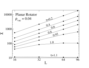
Figure 3: Log-log plot of susceptibility versus system edge length $L$, for the PRM at 4% vacancy concentration. The curves correspond to different values of the dimensionless temperature $\tau=k_{B}T/JS^{2}$. Lines are guides to the eye; errors are smaller than the symbols. Least squares fits were used to determine the slopes, $(2-\eta)$, producing $\eta(T)$ as seen in Fig. 4.

According to renormalization-group theory, the helicity modulus in an infinite system jumps from the finite value $(2/\pi)k_{B}T_{c}$ to zero at the critical temperature. Assuming this applies also to the spin-diluted model, as argued in Ref. Leonel+03, , $T_{c}$ can be estimated from the intersection of $\Upsilon(T)$ and the straight line,

$$\Upsilon=\frac{2}{\pi}k_{B}T.$$ (9)

The trend in the intersection point with increasing $L$ can be observed, as shown for the PRM at $\rho_{\textrm{vac}}=0.04$ in Fig. 2. Generally speaking, the MC data for $\Upsilon(T)$ show a steeper drop in the critical region as $L$ increases. The larger system size used, the lower will be the intersection point and estimated $T_{c}$. Hence this method will always lead to an over-estimate of $T_{c}$.

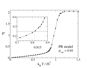
Figure 4: Application of the correlation exponent $\eta$ for estimating $T_{c}$, for the PRM at 4% vacancy concentration, derived from using systems of sizes $L=16,32,64,96$. The inset shows how the critical temperature was estimated as $k_{B}T_{c}/JS^{2}\approx 0.815$.

Finally a third approach was also applied for estimating $T_{c}$, employing the finite size scaling of the in-plane susceptibility, as used in a pure XXZ model by Cuccoli et al.Cuccoli+95 and in the same model with repulsive vacancies by Wysin. Wysin05 In the absence of vacancies, it is the most precise method, because the statistical fluctuations in $\chi$ can be reduced by extended MC averaging much more effectively than those of the helicity modulus or Binder’s cumulant. We assume that near and below $T_{c}$, a power law scaling of the susceptibility holds, even in the presence of vacancies,

$$\chi\propto L^{2-\eta},$$ (10)

where $\eta$ is the exponent for the in-plane spin correlations below $T_{c}$ (see Ref. Cuccoli+95, ). By using this equation with calculations at several lattice sizes, the exponent $\eta$ can be fitted as a function of temperature. An indication of how $\chi$ scales with system size is given in Fig. 3, again for the PRM at 4% vacancy concentration. One can note clearly how the exponent $(2-\eta)$ (slope of log-log plot for $\chi(L)$) decreases as the temperature increases, especially rapidly as $T$ passes the transition temperature.

For the pure PR and XY models (no vacancies), the transition is located at the temperature where $\eta(T)=1/4$. Then, under that assumption that the vacancies do not change the basic symmetries in the transition, but only increase the effective entropy present, we can expect that the transition can be located in the same way under the presence of vacancies, solving

$$\eta(T_{c})=\frac{1}{4}.$$ (11)

In the absence of any particular theory for the model with vacancies, this can be expected to be a reasonable definition for $T_{c}$. Analysis of power-law fits of the spin-spin correlations in the diluted PRM Berche+03 also demonstrated that $T_{c}$ occurs very close to the temperature from Eq. (11). Its validity is further verified here by the comparison with the results for $T_{c}$ due to the helicity modulus, and due to Binder’s cumulant, the latter of which is reliable for any kind of model, with or without vacancies. Fig. 4 shows its application for the PRM at 4 % vacancy concentration, leading to $k_{B}T_{c}/JS^{2}\approx 0.815$, exactly consistent with the estimate from Binder’s cumulant (Fig. 1).

We also note, that for the pure PRM (no vacancies), this fitting of $\eta$, using systems as large as $L=160$, leads to the estimate $k_{B}T_{c}/JS^{2}=0.907\pm 0.004$, slightly higher than that from Ref. Tobochnik79, .

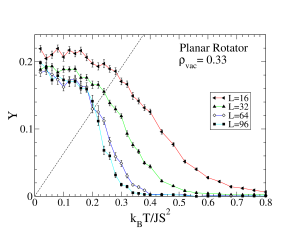
Figure 5: The helicity modulus for the PRM at 33% vacancy concentration for system sizes indicated. The dashed line is Eq. (9).

Figure 6: Binder’s fourth cumulant for the PRM at 33% vacancy concentration for system sizes indicated. $k_{B}T_{c}/JS^{2}\approx 0.14$ as estimated from the point where the data for different system sizes separate. The lines are guides to the eye.

II.2 Monte Carlo Scheme

Thermal averages for a given system size and temperature were obtained using a hybrid MC approach, including Metropolis single-spin moves and over-relaxation movesEvertz96 that can modify all spin components, in combination with Wolff single-cluster movesWolff88 ; Wolff89 that modify only the xy components. These are based on standard approaches for spin models, as developed in many references.Kawabata+86a ; Kawabata+86b ; Wysin90 ; Gouvea97 ; Landau99 Further details, as applied to a system with vacancies, can be found in Ref. Wysin05, . Using a hybrid method including cluster and over-relaxation is very important especially at low temperatures, as it very effectively reduces the problems associated with critical slowing down.

The programming used for the XY model also applies to the planar rotator model; it is only necessary to set the out-of-plane components $S^{z}=0$ and then never allow them to change for the PRM. Thus it is straightforward to study the two models with essentially the same MC approach.

The calculations were performed for a range of system sizes, including $L=16,32,64,96,$ and $160$. For a given $L\times L$ lattice, the number of vacancies placed at random locations was $N_{\textrm{vac}}=\rho_{\textrm{vac}}L^{2}$ (spins removed from system or equivalently, set to zero length). For larger systems or very low vacancy density, the results are nearly independent of the particular random choice of vacancy positions. In the general case, however, it is necessary to average over equivalent systems (same $L$, $\rho_{\textrm{vac}}$) with different particular choices of the vacancy locations. The statistical variations in the averages are most significant especially as the vacancy density approaches the critical value that forces $T_{c}$ to zero. These statistical variations also are strongest in the smaller systems; conversely, the larger systems tend to average out these fluctuations, all the better as their area increases. Therefore we averaged over a number $N_{\textrm{sys}}$ copies of the system, with this number taken largest at small system size. For $\rho_{\textrm{vac}}<0.35$, we used $N_{\textrm{sys}}=64,32,8,4,$ for $L=16,32,64,96$, respectively. For larger density, $\rho_{\textrm{vac}}>0.35$, we doubled these values for $N_{\textrm{sys}}$, and additionally included runs with $N_{\textrm{sys}}=4$ for $L=160$.

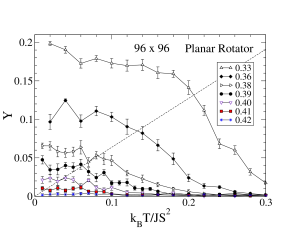
Figure 7: The helicity modulus for the PRM at vacancy concentrations $\rho_{\textrm{vac}}$ indicated in the legend. The dashed line is Eq. (9). Part (a) shows the overall trend; error bars are smaller than the symbols. Part (b) displays the behavior as the transition is extinguished at the critical vacancy concentration.

For thermal equilibration before calculating averages, $5000$ MC steps (MCS) were applied for small systems ($L<50$) and $10,000$ MCS for large systems. For each of the $N_{\textrm{sys}}$ individual realizations of a given $L$ and $\rho_{\textrm{vac}}$, averages at one temperature were calculated using between 20,000 and 80,000 MCS ($N_{\textrm{data}}$), with the greatest number applied to the larger systems. For example, calculation for one temperature of a $16\times 16$ lattice at $\rho_{\textrm{vac}}=0.1$ involved an average over $64\times 25,000=1.28$ million MCS. On the other hand, one temperature of a $96\times 96$ lattice at $\rho_{\textrm{vac}}=0.36$ involved an average over $8\times 80,000=640,000$ MCS. Near 0% vacancy density, these MC parameters produce insignificant error bars; when $\rho_{\textrm{vac}}$ exceeds 30%, on the other hand, the resulting error bars are considerably greater and resist reduction. As suggested above, the error bars in $\Upsilon$, $\chi$, and $U_{L}$ can be reduced more readily by increasing $N_{\textrm{sys}}$ than by increasing $N_{\textrm{data}}$ when significant vacancy density is present (especially at $\rho_{\textrm{vac}}>0.3$).

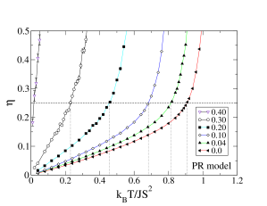
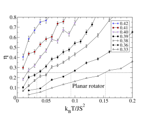
Figure 8: Application of the correlation exponent $\eta$ for estimating $T_{c}$, for the PRM at the vacancy concentrations indicated in the legend, derived from scaling of $\chi$ for systems of sizes $L=16,32,64,96$. Part (a) gives the rough overall trend and part (b) shows how $\eta$ does not fall to the value $1/4$ at vacancy concentrations greater than 41%.

III Monte Carlo Data

Calculations were carried for a range of vacancy densities from zero to 50%. We especially concentrated on the region $0.30<\rho_{\textrm{vac}}<0.40$, which required the most careful analysis. For vacancy density less than 30%, it is clear that there is a transition at a finite temperature, for both the PR and XY models. At the higher vacancy concentrations, statistical errors were generally more significant. Even so, looking at the trends in the data with system size, in the following we show the MC evidence that the transition temperature is reduced to zero when the vacancy concentration is approximately 40%, for both models.

III.1 Planar rotator model

At low vacancy concentrations ($\rho_{\textrm{vac}}<0.20$), MC results for $U_{L}$, $\Upsilon$, $\chi$, and $\eta(T)$ bear a great resemblance to those shown above for 4% vacancies, with fairly smooth dependencies on temperature. The primary modification is the general trend of important features towards lower temperature with increasing $\rho_{\textrm{vac}}$. At higher concentrations, errors become more significant. For example, the helicity modulus at 33% vacancies and various system sizes is shown in Fig.  5. In addition to larger relative errors, the absolute magnitude of $\Upsilon$ is drastically reduced. It is very clear, however, that the BKT transition is still present at this concentration, with $k_{B}T_{c}/JS^{2}\approx 0.20$ as estimated from the crossing point of the $L=96$ data. This is additionally supported by the corresponding behavior of Binder’s cumulant, seen in Fig. 6, which gives the estimate $k_{B}T_{c}/JS^{2}\approx 0.14$, somewhat lower, as can be expected.

An indication of the tendency for reduction of $T_{c}$ with vacancy concentration is given in Fig. 7, showing a collection of results all for $L=96$ systems. While these crossing points consistently overestimate $T_{c}$, a better view of this critical point reduction is provided by the various graphs of $\eta(T)$ at different concentrations, Fig. 8. One can see clearly that once the vacancy concentration passes a value around 41%, the fitted value of $\eta$ does not fall below the value $1/4$, at least for the lowest temperatures used ($k_{B}T/JS^{2}=0.01$).

In Fig. 9, the critical temperatures extracted from $\eta$ and Eq. (11) and from the helicity modulus (using $L=96$) are shown as functions of vacancy concentration. As mentioned above, the crossing point of $\Upsilon(T)$ with Eq. (9) for any finite system always overestimates $T_{c}$, with less error as larger systems are used. The fitting of $\eta$ is more reliable; the data shown here used the scaling fitting of $\chi$ using systems with sizes $L=16,32,64,96$. The numerical values of $T_{c}$ estimated using $\eta(T_{c})=1/4$ are summarized in Table 1. The results give strong evidence for extinction of the BKT transition at a vacancy concentration close to 41%.

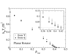
Figure 9: The critical temperatures versus vacancy concentration for the PRM, extracted from fits of $\eta$ together with Eq. (11) and from the crossing of $\Upsilon(T)$ with Eq. (9) for $L=96$ systems. The inset shows $T_{c}$ as $\rho_{\textrm{vac}}$ approaches the critical region.

Table 1: Dependence of dimensionless critical temperature $\tau_{c}\equiv k_{B}T_{c}/JS^{2}$ on $\rho_{\textrm{vac}}$, as derived from the scaling of in-plane susceptibility $\chi$, and using $\eta(T_{c})=1/4$.

$\rho_{\textrm{vac}}$	$\tau$ (PR model)	$\tau$ (XY model)
0.0	$0.907\pm 0.004$	$0.700\pm 0.005$
0.04	$0.815\pm 0.005$	$0.637\pm 0.005$
0.10	$0.683\pm 0.004$	$0.547\pm 0.005$
0.16	—	$0.453\pm 0.005$
0.20	$0.456\pm 0.004$	$0.384\pm 0.005$
0.30	$0.230\pm 0.004$	$0.208\pm 0.005$
0.33	$0.153\pm 0.007$	$0.147\pm 0.005$
0.36	$0.093\pm 0.005$	$0.087\pm 0.005$
0.38	$0.050\pm 0.006$	$0.049\pm 0.005$
0.39	$0.034\pm 0.006$	$0.041\pm 0.005$
0.40	$0.019\pm 0.009$	$0.018\pm 0.007$
0.41	$0.005\pm 0.009$	$0.003\pm 0.007$
0.42	$0.0\pm 0.005$	$0.0\pm 0.005$
0.44	$0.0\pm 0.005$	$0.0\pm 0.005$

III.2 XY model

The general trends in MC data for the XY model are rather similar to those found for the planar rotator. The most obvious distinction, however, is that the extra entropy due to the out-of-plane spin component forces the transition temperature to be lower in the XY model, no matter what vacancy concentration is considered.

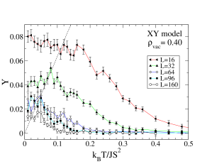
Figure 10: The helicity modulus for the XY model at 40% vacancy concentration for system sizes indicated. The dashed line is Eq. (9).

It is interesting to show some data at 40% vacancy concentration, where the transition is seen to occur very slightly above zero temperature. In Fig. 10 the helicity modulus for system sizes from $L=16$ to $L=160$ is displayed. As the data for increasing system size is seen to systematically fall to lower values, this graph alone cannot undeniably prove the presence of a transition. However, when taken in conjunction with the fits for $\eta$, which passes the value $1/4$ around $k_{B}T/JS^{2}\approx 0.018$, we can say that even at 40% vacancy density there occurs a transition at finite temperature. This can be seen in Fig. 11, where $\eta(T)$ is shown for the various vacancy concentrations studied. On the other hand, performing the MC calculations at temperatures as low as $k_{B}T/JS^{2}=0.01$, the exponent $\eta$ does not acquire such a low value as $1/4$ even for 41% vacancy concentration.

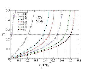
Figure 11: Application of the correlation exponent $\eta$ for estimating $T_{c}$, for the XY model at the vacancy concentrations indicated in the legend, derived from scaling of $\chi$ for systems of sizes $L=16,32,64,96$. Part (a) gives the rough overall trend and part (b) shows how $\eta$ does not fall to the value $1/4$ at vacancy concentrations greater than 41%.

Figure 12: The critical temperatures versus vacancy concentration for the XY model, extracted from fits of $\eta$ together with Eq. (11) and from the crossing of $\Upsilon(T)$ with Eq. (9) for $L=96$ systems. The inset shows $T_{c}$ as $\rho_{\textrm{vac}}$ approches the critical region.

In Fig. 12, the critical temperatures extracted from $\eta$ and Eq. (11) and from the helicity modulus (using $L=96$) are shown as functions of vacancy concentration. The numerical values as derived using $\eta(T_{c})=1/4$ are given in Table 1. Just as in the PR model, these results demonstrate the extinction of the BKT transition at a vacancy concentration close to 41%. As the transition is controlled by the in-plane spin components, the presence of the extra $S^{z}$ component in the XY model changes the overall scale of transition temperatures, but does not affect the critical vacancy concentration.

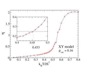
Figure 13: Application of the correlation exponent $\eta$ for estimating $T_{c}$, for the XY model at 16% vacancy concentration, derived from using systems of sizes $L=16,32,64,96$. The inset shows how the critical temperature was estimated as $k_{B}T_{c}/JS^{2}\approx 0.453$.

Finally, we can also make some comparison to the XY model using repulsive vacancies studied in Ref. Wysin05, . Considerable data was presented there for the case of 16% vacancies. Therefore it is interesting to note how the transition temperature is changed if the vacancies are allowed to be at completely random positions in the current model.

A graph of $\eta(T)$ for this case is given in Fig. 13, showing clearly the transition occurring at $k_{B}T_{c}/JS^{2}\approx 0.453$. Alternatively, and even with less computational effort, the transition can be found as done in Refs. Cuccoli+95, ; Wysin05, by plotting $\chi/L^{(2-\eta)}$ vs. $T$, taking $\eta=1/4$, and looking for the common crossing point of data at various system sizes. This is seen in Fig. 14, which gives the same estimate for $T_{c}$. In the repulsive vacancy model at the same vacancy concentration, the transition occurs at a slightly higher temperature, $k_{B}T_{c}/JS^{2}\approx 0.478\pm 0.001$. The result is reasonable; there is greater disorder in the model with fully random vacancies, hence, requiring less thermal disordering due to temperature to reach the high-temperature phase. (alternatively, the repulsive vacancy model has more built-in order and hence requires greater thermal energy per spin to reach the high-temperature phase.)

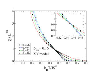
Figure 14: Application of the finite-size scaling of in-plane susceptibility $\chi$ to estimate $k_{B}T_{c}/JS^{2}\approx 0.453$ (common crossing point of the data) at 16% vacancy density in the XY model, with fully randomly placed vacancies, using exponent $\eta=1/4$.

IV Conclusions

Hybrid MC calculations applied to the planar rotator and XY models on a 2D square lattice show that the BKT transition is extinguished ($T_{c}\to 0$) at a vacancy concentration close to 41%, a number related to the percolation limit. Then, although the BKT phase transition has an unusual nature, in which the topological long-range order is destroyed by the unbinding of vortices, the percolation problem of systems exhibiting such a transition must have some similarities to the traditional $2D$ Ising model. In general, the transition temperatures for the XY model are lower than those for the PR model, due to the extra entropy of out-of-plane spin motions, but otherwise, the static properties are closely related. The transition temperatures were determined most precisely using the finite-size scaling of the in-plane magnetic susceptibility, under the assumption that the spin-correlation exponent $\eta$ goes to the universal value $1/4$ at the transition, regardless of the vacancy concentration. This is equivalent to saying that the presence of spin vacancies does not change any fundamental symmetries of the problem. $T_{c}$ calculated this way is completely consistent with the corresponding results from the helicity modulus and Binder’s fourth order cumulant. At vacancy concentration higher than 41%, the intrinsic disorder of the system always produces a phase with short range correlations that decay exponentially, i.e., the usual “high-temperature” BKT phase whose properties are strongly determined by the presence of unbound vortices and antivortices. The lack of percolation across the system at $\rho_{\textrm{vac}}>0.41$ disrupts the ability to generate topological long-range correlations. It then becomes impossible to lower the temperature adequately to reach the ordered phase of very low vortex density, dominated by spin waves.

- (1) V.L. Berezinskii, Sov. Phys. JEPT 32, 493 (1970).
- (2) V.L. Berezinskii, Sov. Phys. JEPT 34, 610 (1972).
- (3) J.M. Kosterlitz and D.J. Thouless, J. Phys. C 6, 1181 (1973).
- (4) J. Tobochnik and G.V. Chester, Phys. Rev. B 20, 3761 (1979).
- (5) A. Cuccoli, V. Tognetti, and R. Vaia, Phys. Rev. B 52, 10221 (1995).
- (6) H.G. Evertz and D.P. Landau, Phys. Rev. B 54,12302 (1996).
- (7) K. Subbaraman, C.E. Zaspel, J.E. Drumheller, Phys. Rev. Lett. 80, 2201 (1998).
- (8) C.E. Zaspel, C.M. McKennan, and S.R. Snaric, Phys. Rev.B 53, 11317 (1996).
- (9) M.M. Bogdan and C.E. Zaspel, Phys. Status Solidi A 189, 983 (2002).
- (10) A.R. Pereira, A.S.T. Pires, J. Magn. Magn. Mater. 257, 290 (2003).
- (11) A.R. Pereira, L.A.S. Mól, S.A. Leonel, P.Z. Coura, and B.V. Costa, Phys. Rev. B 68, 132409 (2003).
- (12) G.M. Wysin, Phys. Rev. B 68, 184411 (2003).
- (13) F.M. Paula, A.R. Pereira, L.A.S.Mól, Phys. Lett.A 329, 155 (2004).
- (14) A.R. Pereira, S.A. Leonel, P.Z. Coura, and B.V. Costa, Phys. Rev.B 71, 014403 (2005).
- (15) H. Karatsuji and H. Yabu, J. Phys. A 29, 6505 (1996).
- (16) L.A.S. Mól, A.R. Pereira, W.A. Moura-Melo, Phys. Rev. B 67, 132403 (2003).
- (17) A.R. Pereira, J. Mag. Magn. Mater. 279,396 (2004).
- (18) S.A. Leonel, P.Z. Coura, A.R. Pereira, L.A.S. Mól, and B.V. Costa, Phys. Rev. B67104426 (2003).
- (19) B. Berche, A.I. Fariñas-Sánches, Y. Holovatch, and R. Paredes, Eur. Phys. J. B. 36,91 (2003)
- (20) G.M. Wysin, to appear in Phys. Rev. B (2005).
- (21) L.M. Castro, A.S.T. Pires, and J.A. Plascak, J. Mag. Mag. Mater. 248,62 (2002).
- (22) Y.E. Lozovick and L.M. Pomirchi, Phys. Sol. State 35, 1248 (1993).
- (23) K. Binder, Z. Phys. B 43,119 (1981).
- (24) V. Privman, ed., Finite Size Scaling and Numerical Simulation of Statistical Systems (World Scientific Publishing, Singapore, 1990).
- (25) U. Wolff, Nucl. Phys. B 300,501 (1988).
- (26) U. Wolff, Phys. Rev. Lett. 62,361 (1989).
- (27) C. Kawabata, M. Takeuchi, and A.R. Bishop, J. Magn. Magn. Mater. 54-57, Pt.2, 871 (1986).
- (28) C. Kawabata, M. Takeuchi, and A.R. Bishop, J. Magn. Magn. Mater. 54-57, Pt.2, 871 (1986).
- (29) G.M. Wysin and A.R. Bishop, Phys. Rev. B 42, 810 (1990).
- (30) M.E. Gouvêa and G.M. Wysin, Phys. Rev. B 56, 14192 (1997).
- (31) D.P. Landau, J. Magn. Magn. Mater. 200,231 (1999).