Thermodynamic origin of order parameters in mean-field models of spin glasses

Abstract

We analyze thermodynamic behavior of general $n$-component mean-field spin glass models in order to identify origin of the hierarchical structure of the order parameters from the replica-symmetry breaking solution. We derive a configurationally dependent free energy with local magnetizations and averaged local susceptibilities as order parameters. On an example of the replicated Ising spin glass we demonstrate that the hierarchy of order parameters in mean-field models results from the structure of inter-replica susceptibilities. These susceptibilities serve for lifting the degeneracy due to the existence of many metastable states and for recovering thermodynamic homogeneity of the free energy.

I Introduction

An effective spin exchange between magnetic impurities diluted in a host metallic matrix is inhomogeneous and does not prefer either ferromagnetic or antiferromagnetic alignment of the impurity spins. It is hence natural to simulate such a magnetic behavior by a random distribution of the spin exchange as introduced by Edwards and Anderson.Edwards75 Frustration in the spin exchange induced by static randomness has since then become the hallmark of microscopic models of spin glasses. Due to complexity of spin-glass models, majority of theoretical research of spin glasses has concentrated on mean-field properties of the Ising spin glass proposed by Sherrington and Kirkpatrick.Sherrington75 ; Binder86 Although we have by now a consistent comprehensive solution of the Sherrington-Kirkpatrick (SK) model in form of the replica-symmetry breaking (RSB) scheme of Parisi,Parisi80 there remain a few issues where a conclusive answer is still pending.

One of unsettling features in spin-glass models is the way the mean-field solution and its interpretation are obtained. On one hand, the replica trick and replicas of the spin variables are used to convert the static randomness to a dynamical, thermal-like averaging and to offer a necessary space for introduction of symmetry breaking order parameters. They are overlaps between different spin replicas $Q^{ab}=N^{-1}\sum_{i}\langle S_{i}^{a}S_{i}^{b}\rangle$. The brackets denote joint thermal and configurational averaging. The physical interpretation of the replica order parameters can, however, be reached only within a thermodynamic approach where a mean-field free energy is first constructed for typical configurations of the spin-exchange. In this thermodynamic approach pioneered by Thouless, Anderson and Palmer (TAP)Thouless77 we have only local magnetizations $m_{i}=\langle S_{i}\rangle_{T}$, thermally averaged local spins, as order parameters for the Ising spin glass. To complete the mean-field solution, a relation between the local magnetizations from the TAP approach and the averaged replica parameters must be established. It was successfully done within the so-called cavity method with many metastable TAP states.Mezard86 ; Mezard87

The existence of a multiple of solutions to the TAP equations has been demonstrated both directlyBray79 ; Cavagna04 and also indirectly.Bray80 ; Cavagna03 Within the cavity method the parameters $q^{\alpha\beta}=N^{-1}\sum_{i}m_{i}^{\alpha}m_{i}^{\beta}$, overlaps between local magnetizations from different pure (metastable) states, were related to the RSB parameters $Q^{ab}$. However, the order parameters from the RSB construction can generally be represented as $Q^{ab}=\chi^{ab}+q^{ab}$ where $q^{ab}=N^{-1}\sum_{i}m_{i}^{a}m_{i}^{b}$ is the overlap of local magnetizations between different spin replicas (should not be identified with different metastable states) and $\chi^{ab}=N^{-1}\sum_{i}(\langle S_{i}^{a}S_{i}^{b}\rangle_{T}-m_{i}^{a}m_{i}^{b})$ is the local overlap susceptibility. It is just only the special case of the non-replicated Ising model ($S_{i}^{2}=1$) where the overlap susceptibility in the TAP construction with a single equilibrium state can be expressed via local magnetizations. If we investigate vector spin glassesFischer91 or assume the existence of many quasi-equilibrium states we cannot get rid of local susceptibilities as independent order parameters.

It indeed appears that the local magnetizations $m_{i}$ of the TAP theory fail in determining unambiguously the equilibrium thermodynamic states. It has been demonstrated by numerical means that there is a macroscopic portion of configurations of the spin exchange for which we are either unable to find a stable solution of the TAP equations at low temperaturesBray79 ; Nemoto85 or we have paired stable and unstable solutions with nearly the same energies.Cavagna04 It means that macroscopic parameters, temperature and external magnetic field, do not determine uniquely local magnetizations and it is unclear whether there is an equilibrium TAP state at all temperatures. In such a case the TAP free energy is no longer thermodynamically homogeneous and solutions of the TAP equations depend on initial/boundary conditions. We have to introduce spin replicas and overlap local susceptibilities emerge as natural order parameters.Janis03

The aim of this paper is to trace down the genesis of the order parameters $Q^{ab}$ from the RSB scheme within the thermodynamic TAP-like approach. In particular, we analyze the role of local magnetizations $m_{i}^{a}$ with their averaged overlaps $q^{ab}$ and averaged local susceptibilities $\chi^{ab}$ in the mean-field free energy of a general $n$-component spin-glass model with spin components $S^{a}$, $a=1,\ldots,n$. We employ the replicated TAP theory from Ref. Janis03, as the simplest example of an $n$-component spin model and find that not the local magnetizations and their averaged overlaps $q^{ab}$, but rather the overlap local susceptibilities $\chi^{ab}$ seem to be relevant order parameters in the spin glass phase. To demonstrate this we first analyze two real replicas of Ising spin variables. Using the replica-symmetric ansatz we then continue analytically the replicated TAP free energy to arbitrary replication factors to enable investigation of thermodynamic homogeneity. We recover the one-step RSB solution of Parisi by minimizing thermodynamic inhomogeneity incurred by the imposed replica-symmetry. Conditions for global thermodynamic homogeneity and a way to reach a thermodynamically homogeneous mean-field free energy are presented.

The paper is organized as follows. We define in Sec. II the studied models being generally $n$-component spin systems. Multi-component spin models can arise either due to the vector character of spins or due to replications of the phase space introduced to test thermodynamic homogeneity. We sum in Sec III mean-field thermal fluctuations for a typical configuration of the spin exchange before averaging over randomness. In Sec. IV we analyze the case of two real replicas to demonstrate the importance of the averaged local overlap susceptibility in the spin-glass phase. We analytically continue the replicated free energy from integer numbers of real replicas to arbitrary replication factors in Section V using the replica-symmetric ansatz. Stability conditions and a hierarchical construction of a globally homogeneous solution are presented in Sec. VI. Finally, in Sec. VII we discuss the physical meaning of the order parameters in the replicated phase space and we summarize the conclusions in Sec. VIII.

II Spin-glass models and thermodynamic homogeneity

The Ising spin glass in its mean-field limit, the SK model, is degenerate in that the fluctuation-dissipation theorem allows us to exclude local susceptibilities from the order parameters of the configurationally dependent free energy. We hence will consider general vector spin models so as to assess better the role and importance of local susceptibilities in the mean-field thermodynamics of spin glasses. Our starting Hamiltonian reads

$$\widehat{H}=-\frac{1}{2}\sum_{i\neq j}J_{ij}\vec{S}_{i}\cdot\vec{S}_{j}-\vec{H}\cdot\sum_{i}\vec{S}_{i}\ .$$ (1)

The norm of the spin vectors is fixed and we assume for our purposes that it depends on the number of spin components $n$, that is

$$\vec{S}_{i}\cdot\vec{S}_{i}=\sum_{a=1}^{n}S_{i}^{a}S_{i}^{a}=ns_{n}^{2}\ .$$ (2)

We are interested in the thermodynamic limit of thermodynamic potentials of this Hamiltonian for fixed configurations of the spin-exchange parameters $J_{ij}$. The free energy reads

$$F=-\frac{1}{\beta}\lim_{N\to\infty}\ln\text{Tr}_{S}\left[\exp\left\{\frac{\beta}{2}\sum_{i,j=1}^{N}J_{ij}\vec{S}_{i}\cdot\vec{S}_{j}\right.\right.\\ \left.\left.+\beta\vec{H}\cdot\sum_{i=1}^{N}\vec{S}_{i}\right\}\right]\ .$$ (3)

The trace $\text{Tr}_{S}$ is taken over all admissible spin configuration respecting the normalization condition (2). The free energy in Eq. (3) is very general and covers vector spin models as well as replicated spin models that we will need for the investigation of thermodynamic homogeneity.

Since the ordering part of the spin exchange is irrelevant for our reasoning we assume only purely fluctuating frustrated spin exchange that in the mean-field limit has a long-range character and is a Gaussian random variable with

$$\left\langle J_{ij}\right\rangle_{av}=0,\qquad\left\langle J_{ij}^{2}\right\rangle_{av}=\frac{J^{2}}{N},\qquad\text{for}\quad i\neq j.$$ (4)

The mean-field models are peculiar in that they are long-range with a volume-dependent spin-exchange as in Eq. (4). The volume-dependence just compensates for the infinite range of the spin exchange. Thereby the energy remains linearly proportional to the volume and we can expect that the mean-field solution emulates the thermodynamic properties of realistic models in a sense reliably or at least consistently.

One of fundamental properties of thermodynamic systems is thermodynamic homogeneity. It says that thermodynamic potentials are products of the volume and functions where all extensive variables enter only via their spatial densities. Thermodynamic homogeneity is normally expressed as the Euler lemma

$$\alpha F(T,V,N,\ldots,X_{i},\ldots)\\ =F(T,\alpha V,\alpha N,\ldots,\alpha X_{i},\ldots)$$ (5)

where $\alpha$ is an arbitrary positive number and the set $\{X_{i}\}$ covers all extensive variables, the thermodynamic potential $F$ depends on. Only if this homogeneity condition is fulfilled by thermodynamic potentials we can prove the Gibbs-Duhem relation and the thermodynamic limit does not depend on the shape of the volume and on boundary/initial conditions. The simplest example of a thermodynamically inhomogeneous systems is the classical ideal gas with distinguishable particles (Gibbs paradox).

Thermodynamic homogeneity is a consequence of invariance of the thermodynamic limit of short-range models with respect to scalings (contractions and dilatations) of the phase space. Since the spin-exchange in mean-field models is an extensive variable, it is not á priori evident whether also mean-field models should be thermodynamically homogeneous. The mean-field thermodynamics is well defined if the thermodynamic limit exists. Mean-field thermodynamic potentials must be thermodynamically homogeneous to make the thermodynamic limit meaningful. Scalings in the phase space of mean-field models are nonlinear transformations due to the volume dependence of the spin exchange, therefore they are replaced by replications of the phase-space variables when testing thermodynamic homogeneity. To introduce real replicas we use an identity for integer $\nu$: $\left[\text{Tr}\ e^{-\beta H}\right]^{\nu}=\text{Tr}_{\nu}\exp\left\{\beta\sum\limits_{a=1}^{\nu}H^{\alpha}\right\}=\text{Tr}_{\nu}\exp\left\{\beta\sum\limits_{a=1}^{\nu}\left(\sum_{i,j}J_{ij}S_{i}^{a}S_{j}^{a}+\sum_{i}S_{i}^{a}\right)\right\}$, where each replicated spin variable $S_{i}^{a}$ is treated independently, i. e., the trace operator $\text{Tr}_{\nu}$ operates on the $\nu$-times replicated phase space. The free energy of a $\nu$-times replicated system must be just $\nu$-times the free energy of the non-replicated one. To test robustness of this property we add a small perturbation breaking the replica independence $\Delta H(\mu)=\sum_{i}\sum_{a<b}\mu^{ab}S_{i}^{a}S_{i}^{b}$ to allow replica-symmetry breaking in the system response to this disturbance. The perturbed free energy per replica reads

$$F_{\nu}(\mu)=-\frac{1}{\beta}\ \frac{1}{\nu}\ln\text{Tr}_{S}\left[\exp\left\{-\beta\sum_{\alpha=1}^{\nu}H^{\alpha}\right.\right.\\ \left.\left.-\beta\Delta H(\mu)\right.\bigg{\}}\right.\bigg{]}\ .$$ (6)

If the system is thermodynamically homogeneous and the equilibrium state stable, the result must be independent of the number of real replicas after switching off the perturbation, that is

$$\frac{d}{d\nu}\lim_{\mu\to 0}F_{\nu}(\mu)\equiv 0\ .$$ (7)

This is a quantification of thermodynamic homogeneity of long-range, mean-field models. If this condition is fulfilled the thermodynamic limit and macroscopic quantities are well defined. This is the eventual situation we would like to achieve also in spin-glass models. Equation (7) must hold for the configurationally dependent as well as for the averaged free energy.

Thermodynamic homogeneity expresses invariance of the thermodynamic limit, that is, invariance of the way the number of lattice sites becomes infinite. Both limits $N\to\infty$ and $N^{\prime}=\nu N\to\infty$ generate the same macroscopic equilibrium state in thermodynamically homogeneous systems. Thermodynamic homogeneity can be formulated also in the replica trick, where is is equivalent to invariance of the limit of the number of replicas to zero. If the system is thermodynamically homogeneous then the limits $n\to 0$ and $\nu n\to 0$ must produce the same results. We hence can introduce real replicas also in the replica trick to test thermodynamic homogeneity there.Janis04

III Mean-field theory for $n$-component spin glass models

Models with $n$ independent spin components have the advantage that they can be treated in the same way as their replicated versions. The only difference is in the number of spin components and the way we perform the trace over spins. We hence will not specify the trace operator in this section and keep the result valid for all situations of interest.

A mean-field theory is an approximation where the interacting part of the free energy is replaced by purely local terms. It can be achieved either by a volume-dependent scaling of a long-range exchange as in the SK model or we can consider the limit to infinite dimensions with appropriately rescaled short-range spin exchange in the Edwards-Anderson model. The best way to control a mean-field approximation is to employ a perturbation expansion in the spin exchange $J_{ij}$. The mean-field contribution is then the leading nonvanishing order in the long-range or infinite-dimensional limit. It is easy to verify that spins on distinct lattice sites interact in the mean-field solution of spin-glass models with the normalization of the spin exchange from Eq. (4) only if connected by maximally squares of $J_{ij}$. This property of the mean-field solution can be conveniently represented diagrammatically. Then only trees and simple loops in the spin exchange contribute. Trees represent an inhomogeneous Weiss mean-field while the loops stand for Onsager’s cavity field.

III.1 Tree contribution

Tree contributions in the diagrammatic expansion for the free energy lead to local magnetizations as thermally averaged values of spin variables. We write

$$\vec{S}_{i}=\vec{M}_{i}+\delta\vec{S}_{i}$$ (8)

where $\vec{M}_{i}=\text{Tr}_{S}[\vec{S}_{i}\widehat{\rho}]$, $\widehat{\rho}=\exp\{-\beta\widehat{H}\}/Z$, $\text{Tr}_{S}[\widehat{\rho}]=1$,. is the local magnetization and $\delta\vec{S}_{i}$ is the fluctuating part of the spin vector. We rewrite the free energy as a contribution from local magnetizations and fluctuating spins

$$F=-\frac{1}{2}\sum_{ij}J_{ij}\vec{M}_{i}\cdot\vec{M}_{j}-\vec{H}\cdot\sum_{i}\vec{M}_{i}\\ -\frac{1}{\beta}\ln\text{Tr}_{\delta S}\left[\exp\left\{\frac{\beta}{2}\sum_{ij}J_{ij}\delta\vec{S}_{i}\cdot\delta\vec{S}_{j}\right.\right.\\ \left.\left.+\beta\sum_{i}\delta\vec{S}_{i}\cdot\left(\vec{H}+\sum_{j}J_{ij}\vec{M}_{j}\right)\right\}\right]$$ (9)

where the trace is taken only over spin fluctuations around their thermal averages. Hence, $\text{Tr}_{\delta S}[\delta\vec{S}_{i}\widehat{\rho}]=0$. The Weiss mean-field solution is obtained from Eq. (9) if the quadratic term in spin fluctuations is neglected. Since $J_{ij}^{2}\propto N^{-1}$ we cannot neglect correlations between fluctuating spin components in spin-glass models.

III.2 One-loop contribution

To derive the leading loop corrections to the inhomogeneous Weiss mean field we reformulate the problem in Gaussian fluctuating fields. We can represent free energy (9) with Gaussian fluctuating fields as follows

$$F=-\frac{1}{2}\sum_{ij}J_{ij}\vec{M}_{i}\cdot\vec{M}_{j}-\vec{H}\cdot\sum_{i}\vec{M}_{i}+\frac{1}{\beta}\ln Z_{0}\\ -\frac{1}{\beta}\ln\left[\int D\Phi\exp\left\{-\frac{1}{2}\sum_{ij}\vec{\Phi}_{i}\cdot W_{ij}\vec{\Phi}_{j}\right\}\right.\\ \left.\text{Tr}_{\delta S}\exp\left\{\sum_{i}\delta\vec{S}_{i}\cdot\left(\vec{\Phi}_{i}+\beta\vec{H}+\sum_{j}\beta J_{ij}\vec{M}_{j}\right)\right\}\right]$$ (10)

where $Z_{0}=\int D\Phi\exp\left\{-\frac{1}{2}\sum_{ij}\vec{\Phi}_{i}\cdot W_{ij}\vec{\Phi}_{j}\right\}$, $\int D\Phi=\prod_{i}\prod_{a}\int_{-\infty}^{\infty}d\Phi_{i}^{a}/\sqrt{2\pi}$, and $\widehat{W}=\widehat{J}^{-1}$. We use hats for operators (matrices) in the lattice space. Notice that the spin-exchange matrix $\widehat{J}$ only with off-diagonal elements is not invertible. We, however, can introduce a suitable chemical potential $-\kappa\delta_{ij}$ to the spin exchange so that $\widehat{J}_{\kappa}=-\widehat{\kappa}+\widehat{J}$ is invertible. It will become evident from the construction that the result at the end will be independent of this artificial chemical potential.

Free energy (10) is difficult in that the trace over the spin fluctuations makes an effective potential for the Gaussian fields $\vec{\Phi}_{i}$ complicated. The potential is, however, local. The one-loop corrections to the Gaussian model can be incorporated in a local self-energy. This self-energy is generally a matrix in the spin components and we denote it $\underline{\sigma}_{i}$. We underline matrices in spin indices. The local self-energy is calculated in a way similar to the cavity method. The procedure is called a generalized coherent potential and was used to derive mean-field theories of quantum itinerant models.Janis89 ; Georges96 The one-loop free energy is that of a Gaussian model with an inhomogeneous, site-diagonal potential $\widehat{\underline{\sigma}}$ into which we embed coherently impurities with the medium potential $\underline{\sigma}_{i}$ replaced by the actual local interaction of the random fields from Eq. (10). It is important that the embedding of impurities is coherent. That is, the fluctuating fields are correlated via local elements of a renormalized exchange of the medium and the effect of the potential $\underline{\sigma}_{i}$ is locally the same as that of the active interaction. It means that if we remove a site $i$ from the Gaussian model with a local potential $\underline{\sigma}_{i}$ and replace it with the local interaction between the fluctuating fields from the original free energy, there is no macroscopic change to be observed.

To perform this task quantitatively we first renormalize the nonlocal correlation matrix $\widehat{W}\to\widehat{W}-\underline{\widehat{\sigma}}$. Although the bare propagator $\widehat{W}$ is diagonal in spin components, the self-energy, as an interaction-induced response to the symmetry-breaking term $\Delta H(\mu)$ can become a nontrivial matrix in spin indices even after switching off the perturbation $\mu^{ab}\to 0$. We introduce local response matrices $\underline{C}_{ii}=\left[(\widehat{W}-\underline{\widehat{\sigma}})^{-1}\right]_{ii}$ containing the correlation between the local sites with fluctuating fields and the surrounding medium of the Gaussian model. Since we have to remove the potential $\underline{\sigma}_{i}$ at the active sites, the effective exchange between the active locally fluctuating fields will be $\widehat{W}\to\underline{C}_{ii}^{-1}+\underline{\sigma}_{i}$ where the inversion is restricted to the chosen lattice site. The one-loop free energy then reads

$$F=-\frac{1}{2}\sum_{ij}J_{ij}\vec{M}_{i}\cdot\vec{M}_{j}-\vec{H}\cdot\sum_{i}\vec{M}_{i}\\ +\text{Tr}\ln(1-\underline{\widehat{\sigma}}\beta\widehat{J})-\frac{1}{\beta}\sum_{i}\ln\int D\Phi\\ \times\exp\left\{-\frac{1}{2}\vec{\Phi}\cdot\underline{C}_{ii}[1+\underline{\sigma}_{i}\underline{C}_{ii}]^{-1}\Phi\right\}\\ \text{Tr}_{\delta S}\exp\left\{\delta\vec{S}_{i}\cdot\left(\vec{\Phi}+\beta\vec{H}+\sum_{j}\beta J_{ij}\vec{M}_{j}\right)\right\}\ .$$ (11)

All introduced local thermodynamic variables $\vec{M}_{i}$, $\underline{\sigma}_{i}$, and $\underline{C}_{ii}$ enter the free energy as variational parameters and are determined from the respective stationarity equations.Janis89

We can now perform the integration over the fluctuating Gaussian fields $\vec{\Phi}_{i}$ and return to the trace with full spins. We obtain

$$F=\frac{1}{2}\sum_{ij}J_{ij}\vec{M}_{i}\cdot\vec{M}_{j}-\frac{1}{2\beta}\sum_{i}\vec{M}_{i}\cdot[\underline{C}_{ii}^{-1}+\underline{\sigma}_{i}]^{-1}\vec{M}_{i}\\ +\frac{1}{2\beta}\text{Tr}\ln(1-\underline{\widehat{\sigma}}\beta\widehat{J})+\frac{1}{2\beta}\sum_{i}\text{Tr}\ln[1+\underline{\sigma}_{i}\underline{C}_{ii}]\\ -\frac{1}{\beta}\sum_{i}\ln\left[\text{Tr}_{S}\exp\left\{\frac{1}{2}\vec{S}_{i}\cdot[\underline{C}_{ii}^{-1}+\underline{\sigma}_{i}]^{-1}\vec{S}_{i}\right.\right.\\ \left.\left.\vec{S}_{i}\cdot\left(\beta\vec{H}+\sum_{j}\beta J_{ij}\vec{M}_{j}-[\underline{C}_{ii}^{-1}+\underline{\sigma}_{i}]^{-1}\vec{M}_{i}\right)\right\}\right]\ .$$ (12)

We can interpret the individual terms in the mean-field free energy (12) straightforwardly. The first term is the energy due to local magnetizations. The second term is a self-interaction of local magnetizations due to Onsager’s cavity filed. The third term is the free energy of a Gaussian model with a potential $\widehat{\underline{\sigma}}$. The fourth term is a subtraction of local sites from the Gaussian medium on which the spins interact with both the Weiss and Onsager’s fields contained in the last term.

Free energy (12) is an approximate solution where all tree and one-loop diagrams have been summed. Such an approximation becomes exact in the long-range limit with condition (4) or in infinite dimensions with $\langle J_{ij}^{2}\rangle_{av}=J^{2}/2d$.Janis89 In this limit we can further simplify this representation, in particular the nonlocal contribution from the Gaussian model. We do it diagrammatically (expansion in the spin exchange). Instead of summing the contributions from the spin exchange in the logarithm we find the mean-field form of the local correlation function. We have

$$\underline{C}_{ii}=-\frac{\delta}{\delta\underline{\sigma}_{i}}\ln(1-\underline{\widehat{\sigma}}\beta\widehat{J})=\left[\beta\widehat{J}(1-\underline{\widehat{\sigma}}\beta\widehat{J})^{-1}\right]_{ii}\ .$$ (13)

Once we find an appropriate representation for the diagonal elements of the correlation function $\underline{C}_{ii}$ we integrate it back to obtain a representation of the logarithm.

We know that in the mean-field spin-glass model with Eq. (4) distinct lattice sites are connected by just two bonds $J_{ij}^{2}$. We then have to create couples of spin exchanges in the expansion of $\underline{C}_{ii}$ to which we ascribe identical lattice coordinates. When lattice sites $i,j$ are interconnected by $J_{ij}^{2}$ there is no further correlation between these sites. If we fix one site index, the other one contributes only as an average over the lattice. Not to go beyond the one-loop approximation, contractions connecting spin couplings with identical lattice coordinates must not cross and only contractions within contractions can take place (non-crossing approximation). The self energy renormalized by all single loop contributions becomes a new vertex function. We can represent this renormalization self-consistently as

$$\underline{\chi}_{ii}=\underline{\sigma}_{i}\left[1-\underline{\sigma}_{i}\sum_{j}\beta^{2}J_{ij}^{2}\underline{\chi}_{jj}\right]^{-1}\ .$$ (14)

With this result the correlation function $\underline{C}_{ii}$ reads

$$\underline{C}_{ii}=\sum_{j}\beta^{2}J_{ij}^{2}\underline{\chi}_{jj}\left[1-\underline{\sigma}_{i}\sum_{j}\beta^{2}J_{ij}^{2}\underline{\chi}_{jj}\right]^{-1}\ .$$ (15)

Using Eqs. (14) and (15) we obtain the mean-field limit of the nonlocal logarithm from Eq. (12)

$$\text{Tr}\ln(1-\underline{\widehat{\sigma}}\beta\widehat{J})=\frac{1}{2}\sum_{ij}\beta^{2}J_{ij}^{2}\text{Tr}[\underline{\chi}_{ii}\underline{\chi}_{jj}]\\ +\sum_{i}\text{Tr}\ln\left(1-\underline{\sigma}_{i}\sum_{j}\beta^{2}J_{ij}^{2}\underline{\chi}_{jj}\right)$$ (16)

where the first term on the right-hand side is a compensation for the $\underline{\sigma}$-dependence of $\underline{\chi}$. We can replace the nonlocal logarithm in Eq. (12) by the right-hand side of Eq. (16). We then have to add the new local vertex functions $\underline{\chi}_{ii}$ to the variational parameters and obtain a mean-field free energy for multi-component spin-glass models.

The phase space with thermodynamic parameters $\vec{M}_{i}$, $\underline{\sigma}_{i}$, $\underline{C}_{ii}$, and $\underline{\chi}_{ii}$ is unnecessarily large. We can explicitly utilize the solutions of stationarity equations for $\underline{\sigma}_{i}$ and $\underline{C}_{ii}$ so that all loop quantities are expressed only via the vertex functions $\underline{\chi}_{ii}$. These equations are just Eqs. (14) and (15). Moreover, we realize that the vertex functions $\underline{\chi}_{ii}$ appear in the free energy only in their averaged form and we can introduce new configurationally averaged loop parameters $\beta^{2}J^{2}\underline{\chi}=\sum_{j}\beta^{2}J_{ij}^{2}\underline{\chi}_{jj}$. Using all these simplifications in free energy (12) we finally end up with a generalized TAP free energy for $n$-component spin-glass models

$$F=\frac{1}{2}\sum_{ij}J_{ij}\vec{M}_{i}\cdot\vec{M}_{j}-\frac{\beta J^{2}}{2}\sum_{i}\vec{M}_{i}\cdot\underline{\chi}\vec{M}_{i}\\ +\frac{\beta J^{2}}{4}N\text{Tr}[\underline{\chi}\underline{\chi}]-\frac{1}{\beta}\sum_{i}\ln\left[\text{Tr}_{S}\exp\left\{\frac{\beta^{2}J^{2}}{2}\vec{S}_{i}\cdot\underline{\chi}\vec{S}_{i}\right.\right.\\ \left.\left.+\ \beta\vec{S}_{i}\cdot\left(\vec{H}+\sum_{j}J_{ij}\vec{M}_{j}-\beta J^{2}\underline{\chi}\vec{M}_{i}\right)\right\}\right]\ .$$ (17)

This mean-field free energy is very general and covers the vector spin models as well as replicated models used for investigation of thermodynamic homogeneity.

It is straightforward to find that the saddle-point equation for the averaged vertex reads

$$\underline{\chi}=\frac{1}{N}\sum_{j}\left(\left\langle\vec{S}_{j}\vec{S}_{j}\right\rangle-\vec{M}_{j}\vec{M}_{j}\right)$$ (18)

where the vectors on the right-hand side form a tensor (matrix) in spin components. From this equation we obtain the fluctuation-dissipation theorem for vector spin models

$$\text{Tr}\ \underline{\chi}=\frac{1}{N}\sum_{j}(ns_{n}^{2}-\vec{M}_{j}\cdot\vec{M}_{j})\ .$$ (19)

We see from Eq. (18) that the averaged vertex $\underline{\chi}$ is nothing but an averaged local susceptibility (up to the factor $\beta$). Only in the isotropic case with vanishing off-diagonal elements of $\underline{\chi}$ we get rid of the local susceptibility as an order parameter in the TAP-like free energy. We, however, know that this is not the case either in vector modelsGabay81 or in the replicated Ising spin glass.Janis03

III.3 Configurational averaging

Free energy (17) has not yet the form of a typical mean-field representation, being standardly a single-site theory. To convert the spatially inhomogeneous free energy to a single-site expression we have to average over the spin-exchange configurations. It cannot, however, be done without a few assumptions. First of all, we have to assume that the local magnetizations $\vec{M}_{i}$ and averaged susceptibilities $\underline{\chi}$ describe uniquely thermodynamic equilibrium states. It means that we can find a set of these parameters with which the free energy is minimal. It is the case if the nonlocal susceptibility is nonnegative. That is, the second derivative

$$\frac{\delta^{2}\beta F}{\delta M_{i}^{a}\delta M_{j}^{b}}=-\beta J_{ij}\delta^{ab}+\delta_{ij}\left(\left[\underline{\chi}_{ii}^{-1}\right]^{ab}+\beta^{2}J^{2}\chi^{ab}\right)$$ (20)

has no negative eigenvalues. We denoted $\underline{\chi}_{ii}$ the local susceptibility at site $i$. It is a matrix defined as in Eq. (18) but without averaging over the lattice sites. It is a straightforward task to find that the nonlocal susceptibility, inverse of the matrix from Eq. (20), has nonnegative eigenvalues if a generalized de Almeida-Thouless (AT) condition is fulfilled

$$\text{det}\left(\underline{1}-\frac{\beta^{2}J^{2}}{N}\sum_{i}\underline{\chi}_{ii}^{2}\right)\geq 0\ .$$ (21)

This inequality in fact stands for $n$ conditions $1\geq\beta^{2}J^{2}\lambda_{l}^{2}$ restricting each eigenvalue $\lambda_{l}^{2},l=1,\ldots,n$ of the averaged squared local susceptibility $N^{-1}\sum_{i}\underline{\chi}_{ii}^{2}$.

To average over the random configurations we have to assume that equilibrium states determined by the thermodynamic parameters from free energy (17) are non-degenerate. That is, solutions of the stationarity equations do not depend in the thermodynamic limit on boundary or initial conditions. This condition is essentially equivalent to thermodynamic homogeneity. Further on, we assume equivalence of individual spin components, that is $H^{a}=H$ and $\langle(S_{i}^{a})^{2}\rangle_{T}=s_{n}^{2}$. We then can separate diagonal and of-diagonal matrix elements of the local susceptibility. Due to the fluctuation-dissipation theorem we can represent $\chi^{aa}=(s_{n})^{2}-N^{-1}\sum_{i}(M_{i}^{a})^{2}$. We further introduce the internal magnetic field as an independent random variable

$$\eta_{i}^{a}=\sum_{j}J_{ij}M_{j}^{a}-M_{i}^{a}\sum_{j}\beta J_{ij}^{2}\left(1-(M_{j}^{a})^{2}\right)\\ -\beta J^{2}\sum_{b\neq a}\chi^{ab}M_{i}^{b}\ .$$ (22)

We add $\sum_{i}\vec{M}_{i}\cdot\vec{\eta}_{i}$ to free energy (17) and subtract the same term with $\eta_{i}^{a}$ represented by Eq. (22). We obtain a new representation for the isotropic case

$$F=\frac{N}{4}\beta J^{2}\sum_{a\neq b}(\chi^{ab})^{2}+\sum_{i}\sum_{a=1}^{n}M_{i}^{a}\bigg{[}\eta_{i}^{a}\\ +\frac{\beta J^{2}}{2}\sum_{b\neq a}\chi^{ab}M_{i}^{b}\bigg{]}-\frac{1}{4}\sum_{ij}\sum_{a=1}^{n}\left[2J_{ij}M_{i}^{a}M_{j}^{a}\right.\\ \left.+\beta J_{ij}^{2}\left(s_{n}^{2}-(M_{i}^{a})^{2}\right)\left(s_{n}^{2}-(M_{j}^{a})^{2}\right)\right]\\ -\frac{1}{\beta}\sum_{i}\ln\left[\exp\left\{\frac{J^{2}}{2}\sum_{a\neq b}\chi^{ab}\ \frac{\delta}{\delta\eta_{i}^{a}}\ \frac{\delta}{\delta\eta_{i}^{b}}\right\}\right.\\ \left.\text{Tr}_{S}\exp\left\{\sum_{a=1}^{n}S_{i}^{a}(\beta H+\beta\eta_{i}^{a})\right\}\right]$$ (23)

where apart from $M_{i}^{a}$ and $\chi^{ab}$ also the fluctuating field $\eta_{i}^{a}$ are variational parameters.

One can prove with the assumptions mentioned at the beginning of this subsection that the internal magnetic fields $\eta_{i}^{a}$ are Gaussian random variables with covariance

$$\langle\eta_{i}^{a}\eta_{j}^{b}\rangle_{av}=\delta_{ij}\sum_{l}J_{il}^{2}M_{l}^{a}M_{l}^{b}=J^{2}q^{ab}\delta_{ij}\ .$$ (24)

The local Gaussian fields $\eta_{i}^{a}$ are used to replace averaging over the nonlocal spin exchange $J_{ij}$ To make the mean-field free energy explicit we have to simplify nonlocal terms explicitly dependent on the spin exchange $J_{ij}$ (only linearly) and terms with local random variables that are not manifestly Gaussian. Due to the Gaussian character of both the internal magnetic fields $\eta_{i}^{a}$ and the the spin exchange $J_{ij}$ we obtain

$$\langle M_{i}^{a}\eta_{i}^{a}\rangle_{av}=\sum_{b}\left\langle\frac{\delta M_{i}^{a}}{\delta\eta_{i}^{b}}\right\rangle_{av}\langle\eta_{i}^{b}\eta_{i}^{a}\rangle_{av}$$ (25)

and

$$\langle J_{ij}M_{i}^{a}M_{j}^{a}\rangle_{av}\\ =\frac{J^{2}}{N}\left[\left\langle M_{i}^{a}\frac{\delta M_{j}^{a}}{\delta J_{ij}}\right\rangle_{av}+\left\langle\frac{\delta M_{i}^{a}}{\delta J_{ij}}M_{j}^{a}\right\rangle_{av}\right]\ .$$ (26)

Further on, the nonlocal averaging decays into a product of local averages, since

$$\frac{\delta M_{i}^{a}}{\delta\eta_{i}^{b}}=\beta\chi_{ii}^{ab} ,\qquad\frac{\delta M_{i}^{a}}{\delta J_{ij}}=\beta\sum_{b}\chi_{ii}^{ab}M_{j}^{b}\ .$$ (27)

With the above formulas we can average the free energy over random configuration so that only averaged site-independent order parameters remain. The averaged free energy is a sum of local terms only and we can go over to a free-energy density that, for $n$ component isotropic spin-glass models, reads

$$nf_{n}=\frac{\beta J^{2}}{4}\sum_{a\neq b}\chi^{ab}(\chi^{ab}+2q^{ab})-\frac{\beta J^{2}}{4}\sum_{a=1}^{n}\left((s_{n})^{2}-q^{aa}\right)^{2}\\ -\frac{1}{\beta\sqrt{\det{\underline{q}}}}\int D\eta\exp\left\{-\frac{1}{2}\vec{\eta}\cdot(\underline{q}^{-1})\vec{\eta}\right\}\\ \ln\left[\text{Tr}_{S}\exp\left\{\frac{\beta^{2}J^{2}}{2}\sum_{a\neq b}\chi^{ab}S^{a}S^{b}+\beta\sum_{a=1}^{n}S^{a}(H+\eta^{a})\right\}\right]\ .$$ (28)

We denoted $\int D\eta=\prod_{a=1}^{n}\int_{-\infty}^{\infty}d\eta^{a}/\sqrt{2\pi}$.

The averaged free-energy density (28) is our starting point for the analysis of the role of two types of averaged order parameters: the overlap susceptibilities $\chi^{ab}$ and the overlap magnetizations $q^{ab}$. They are determined from saddle-point (stationarity) equations

$$q^{ab} =\left\langle\text{Tr}_{S}\left[\rho_{\chi}S^{a}\right]\text{Tr}_{S}\left[\rho_{\chi}S^{b}\right]\right\rangle_{\eta}$$ (29a)

$$\chi^{ab} =\left\langle\text{Tr}_{S}\left[\rho_{\chi}S^{a}S^{b}\right]\right\rangle_{\eta}-q^{ab},$$ (29b)

where we denoted $\langle\ldots\rangle_{\eta}$ averaging over the random internal magnetic field $\eta$ and $\rho_{\chi}$ is the appropriate density matrix for thermal averaging over spin configurations. We remind that we assumed equivalence of individual spin components, that is $q^{aa}=q_{0}$ and $\chi^{aa}=s_{n}^{2}-q_{0}$ for $a=1,\ldots,n$.

In general $n$-component spin models, both parameters $q^{ab}$ and $\chi^{a\neq b}$ can become relevant in the low-temperature phase. To demonstrate this explicitly we resort our further analysis only to the replicated Ising spin glass with equivalent replicas, although there are no principal obstacles to extend the reasoning to more complex models.

IV Two real replicas

Free energy (28) can be explicitly evaluated only if we fix the number of real replicas or components of the vector model. The simplest situation is the SK model with two equivalent real replicas, that is, the replicated spin space is isotropic. In this case we have $(S^{a})^{2}=1$, $q^{aa}=q_{0}$, $q^{a\neq b}=q$, and $\chi^{a\neq b}=\chi$. It is then easy to calculate the trace over the replicated spin variables. We arrive at

$$f_{2}=-\frac{\beta}{4}(1-q_{0})^{2}+\frac{\beta\chi}{4}(2q+\chi)\\ -\frac{1}{2\beta}\int\mathcal{D}\xi_{1}\mathcal{D}\xi_{2}\ln 2\left\{e_{+}c_{+}+e_{-}c_{-}\right\}\ .$$ (30)

We set $J=1$ in this expression and use this energy scale throughout the rest of the paper. Further on, we used an abbreviation for the Gaussian differential $\mathcal{D}\phi\equiv{\rm d}\phi\ e^{-\phi^{2}/2}/\sqrt{2\pi}$ and we denoted $e_{\pm}=\exp\{\pm\beta^{2}\chi\}$,
$c_{+}=\cosh\left[\beta\left(2h+\sqrt{q_{0}-q^{2}/q_{0}}\ \xi_{1}+(\sqrt{q_{0}}+q/\sqrt{q_{0}})\xi_{2}\right)\right]$,
$c_{-}=\cosh\left[\beta\left(\sqrt{q_{0}-q^{2}/q_{0}}\ \xi_{1}-(\sqrt{q_{0}}-q/\sqrt{q_{0}})\xi_{2}\right)\right]$.

With the above notation we can write down the stationarity conditions representing the equations for the averaged mean-field order parameters.

$$q_{0} =\left\langle\frac{e_{+}^{2}s_{+}^{2}+e_{-}^{2}s_{-}^{2}}{(e_{+}c_{+}+e_{-}c_{-})^{2}}\right\rangle$$ (31a)

$$q =\left\langle\frac{e_{+}^{2}s_{+}^{2}-e_{-}^{2}s_{-}^{2}}{(e_{+}c_{+}+e_{-}c_{-})^{2}}\right\rangle$$ (31b)

$$\chi =(e_{+}^{2}-e_{-}^{2})\left\langle\frac{1}{(e_{+}c_{+}+e_{-}c_{-})^{2}}\right\rangle$$ (31c)

These equations have a solution $q_{0}=q$ and $\chi=0$ in the high-temperature phase. In the low-temperature (spin-glass) phase if

$$0 >1-\beta^{2}\langle(1-t_{12}^{2})(1-t_{2}^{2})\rangle$$ (32a)

then $$\chi>0$$ and

$$0 >1-4\beta^{2}\left\langle\frac{(1-t_{2}^{2})^{2}}{[1-t_{2}^{2}+e_{-}^{2}(1+t_{2}^{2})]^{2}}\right\rangle$$ (32b)

leads to $\Delta=q_{0}-q>0$. We denoted $t_{2}=\tanh\beta(h+\xi_{2}\sqrt{q_{0}})$ and $t_{12}=\tanh\beta(h+\xi_{1}\sqrt{\Delta(2q_{0}-\Delta)/q_{0}}+\xi_{2}(\sqrt{q_{0}}-\Delta/\sqrt{q_{0}})$. Hence, either of these parameters can become an order parameter in the spin-glass phase. We have to find which one is more relevant for thermodynamic stability.

Numerical analysis and an expansion around the critical temperature show that we cannot comply with both conditions (32) simultaneously. That is, either $\Delta>0$ and the condition in Eq. (32a) does not hold ($\chi=0$), or $\chi>0$ and then inequality (32b) cannot be satisfied ($\Delta=0$). If $\chi=0$, the free energy does not depend on $\Delta$ and we recover the SK solution with $q=0$ and $q_{0}=q_{SK}$. Hence the only way to improve upon the SK solution is to choose $\chi>0$ and $q_{0}=q$. The free-energy density reduces in this case to

$$f_{2R}=-\frac{\beta}{4}(1-q)^{2}+\frac{\beta\chi}{4}(2q+\chi)\\ -\frac{1}{2\beta}\int\mathcal{D}\xi\ln 2\left[e_{+}\cosh(2\beta(h+\xi\sqrt{q}))+e_{-}\right]\ .$$ (33)

It is a straightforward task to solve stationarity equations to functional (33). The temperature dependence of the order parameters is plotted in Fig. 1 and of the free-energy density in Fig. 2.

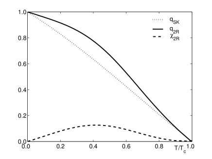
Figure 1: Order parameters for the SK model at zero magnetic field with two real replicas compared to the SK parameter.

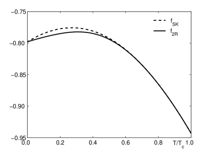
Figure 2: Free energy of the SK model with two real replicas compared to the SK one.

Thermodynamics of the model with two replicas indicates some improvement upon the SK solution. The order parameter $q=\langle m_{i}^{2}\rangle_{av}$ is closer to the Monte-Carlo result.Kirkpatrick78 Entropy at low temperatures is seen from Fig. 2 to be less negative than that of the SK solution. However, the free energy is lower than the SK one, unlike Monte Carlo simulations. At zero-temperature the free-energy density has asymptotics $f_{2R}\doteq-\sqrt{2/\pi}+T/4\pi$. It means that there is no change in the ground-state energy with respect to the SK result. The negative low-temperature entropy of the SK solution is halved with two replicas.

The replicated solution must be unstable. A measure of instability is the generalized AT condition (21). Since we have two replicas, this equation should stand for two conditions. One condition is the complement (negation) to inequality (32b). It is satisfied at any temperature. The second stability condition reads

$$\lambda =1-\beta^{2}\langle X_{2}^{2}(1-t_{2}^{2})^{2}\rangle\geq 0\ ,$$ (34a)

$$X_{2} =2\ \frac{[1-t_{2}^{2}+e_{-}^{2}(1+t_{2}^{2})]}{[1+t_{2}^{2}+e_{-}^{2}(1-t_{2}^{2})]^{2}}$$ (34b)

and is, on the other hand, always broken in the spin-glass phase. When compared with the AT condition of the SK solution, Fig. 3, we can see that the two-replica solution deeper in the low-temperature phase is even less stable than the SK one. The two-replica solution must be modified to improve upon the instability of the SK averaged free-energy density.

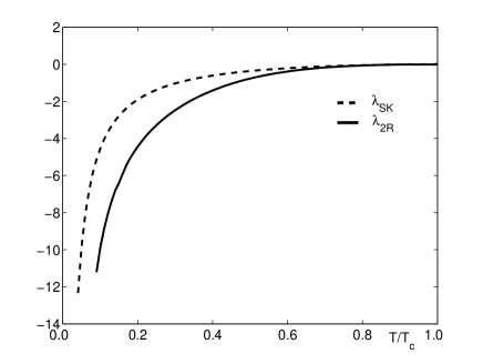
Figure 3: Instability of the two-replica and SK solutions in the spin-glass phase at zero magnetic field.

V Analytic continuation - 1RSB

The most straightforward improvement of the two-replica solution is its extension to an arbitrary number of equivalent real replicas. This can be done explicitly provided $\Delta=0$, that is, $q^{ab}=q$. We show at the end of the next section that the condition for the instability leading to $\Delta>0$ is never fulfilled for integer numbers of real replicas. We hence assume real-replicas with $\Delta=0$. The free-energy density then for a general matrix $\chi^{ab}$ reads

$$f_{n}=\frac{\beta}{4}\left[\frac{1}{n}\sum_{a\neq b}\chi^{ab}\left(\chi^{ab}+2q\right)-(1-q)^{2}\right]\\ -\frac{1}{\beta n}\!\int\limits_{-\infty}^{\infty}\mathcal{D}\eta\ln\text{Tr}_{S}\exp\left\{\frac{\beta^{2}}{2}\sum_{a\neq b}\chi^{ab}S^{a}S^{b}\right.\\ \left.+\beta\sum_{a=1}^{n}S^{a}(H^{a}+\eta\sqrt{q})\right\}\ .$$ (35)

To evaluate explicitly this free energy we assume the replica-symmetric (isotropic) case, $\chi^{ab}=\chi$ for $a\neq b$, and decouple the interacting spins in Eq. (35) by a Hubbard-Stratonovich transformation linearizing the quadratic term in spin variables in the exponential. The trace over the spins can be performed explicitly for arbitrary number of replicas and we obtain a free-energy density with $n$ real replicas

$$f_{n}(q,\chi)\\ =-\frac{\beta}{4}(1-q-\chi)^{2}+\frac{\beta}{4}n\chi(2q+\chi)-\frac{1}{\beta n}\int_{-\infty}^{\infty}\!\!\!\mathcal{D}\eta\\ \times\ln\int_{-\infty}^{\infty}\!\!\!\mathcal{D}\lambda\left\{2\cosh\left[\beta\left(h+\eta\sqrt{q}+\lambda\sqrt{\chi}\right)\right]\right\}^{n}$$ (36)

We can get rid of the $\lambda$-integration from the Hubbard-Stratonovich transformation for any positive integer $n$. It is easy to verify that free energy (36) for $n=2$ reduces to Eq. (33). However, the integral representation of the free energy as used in Eq. (36) is indispensable for analytic continuation of the free energy with integer number of real replicas to an arbitrary real $n$. This continuation is unique if the limit at $|n|\to\infty$ is analytic. The limit to infinite-many replicas exists with $\chi\to\chi^{\prime}/n$. It reduces the $\lambda$-integration to a saddle-point. Free energy analytically continued to arbitrary number of real replicas is a fundamental tool for investigating thermodynamic homogeneity of the solution. According to Eq. (7), thermodynamically homogeneous free energy should not depend on the replication parameter $n$.

We already know that free energy (36) depends on the number of real replicas. The solution cannot hence be thermodynamically homogeneous whatever $n$ we choose. We, however, can use the analytically continued free energy (36) to minimize its inhomogeneity. This minimization is achieved by vanishing of the local dependence of the replicated free energy on the replication factor $n$. That is, we demand

$$\frac{\partial f_{n}}{\partial n}=0\ .$$ (37)

This equation determines the optimal choice of $n$ for which the deviation from thermodynamic homogeneity of the free energy is minimal.

Equation (37) has always a solution. It is easy to verify that $f_{0}=f_{1}=f_{SK}$, whereby for $n=1$ the free energy does not depend on $\chi$ and for $n=0$ we have $q_{SK}=q+\chi$. Hence, there is an $n_{eq}\in[0,1]$ for which Eq. (37) is fulfilled. Moreover, since $f_{n}<f_{SK}$ for $n>1$ and $n<0$, see Fig 4, the solution with the minimal deviation from thermodynamic homogeneity maximizes the free energy as a function of the replication factor $n$.

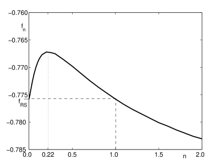
Figure 4: Dependence of the averaged free-energy density on the replication parameter $n$ at $T=T_{c}/4$.

Free energy (36) with the optimized replication parameter $n$ via Eq. (37) is identical with the Parisi 1RSB solution. It significantly improves upon the SK solution in the spin-glass phase. The free energy is higher than the SK one everywhere below the critical point, Fig. 5.

Figure 5: Free-energy density for the optimized replication parameter compared to the SK solution.

Notice that optimization of the replication parameter $n$ via Eq. (37) is a very important constituent of the RSB solution. In particular in low temperatures. The RSB solution improves upon the ground-state energy at zero temperature only if the parameter $n$ depends on temperature. Only if the optimal replication parameter scales with temperature as $n=T\nu$ we obtain nonvanishing overlap susceptibility $\chi$ at zero temperature, Fig. 6, being responsible for a remarkable improvement in the ground-state energy toward the Monte-Carlo result.

Figure 6: Order parameters for 1RSB and two real replicas. We denoted the Parisi parameter $Q=q+\chi$. The importance of optimization of the replication parameter at low temperatures is demonstrated on the behavior of the overlap susceptibility $\chi$.

With $n=T\nu$ we can derive an explicit representation for the zero-temperature free energy

$$f=-\frac{\nu}{4}(1-q)^{2}-\frac{1}{\nu}\int\mathcal{D}\eta\ln A(\eta,\nu,q)\$$ (38)

where we denoted

$$A(\eta,\nu,q)\\ =\left[e^{-\nu\eta\sqrt{q}}\text{erfc}\left(-\nu\sqrt{1-q}+\eta\sqrt{q/(1-q)}\right)\right.\\ \left.+\ e^{\nu\eta\sqrt{q}}\text{erfc}\left(-\nu\sqrt{1-q}-\eta\sqrt{q/(1-q)}\right)\right]\ .$$ (39)

We used the error function $\text{erfc}(x)=\int_{x}^{\infty}e^{-t^{2}/2}dt/\sqrt{\pi}$. The stationarity solution of the zero-temperature free energy can be numerically evaluated rather accurately. We obtain $q=0.477\pm 0.001$, $\nu=1.351\pm 0.001$, and $f=-0.76526\pm 0.00001$. Theory with a fixed number of real replicas leads at low temperatures for whatever fixed $n$ (integer or noninteger) to a solution with $\chi=T\sqrt{2/\pi}/n$, $q=1-\chi$, and $f_{n}=f_{SK}=-\sqrt{2/\pi}+T/2n\pi\approx-0.798$ as found in the preceding section for $n=2$.

VI Stability and hierarchical organization of order parameters

Although the 1RSB solution improves upon the SK results toward the outcome of Monte-Carlo simulations, it is the stability condition (21) that decides whether this could be a final form of the mean-field free energy of the SK model. One-step RSB solution was derived from Eq. (35) with an isotropic or replica-symmetric ansatz on the overlap susceptibilities. The stability condition in this case breaks into two inequalities for two eigenvalues of this solution.

A generalization of the AT stability condition (34) for arbitrary replication number reads

$$\Lambda_{0}=1-\beta^{2}\left\langle\left[1-(1-n)\langle\rho_{n}t^{2}\rangle_{\lambda}-n\langle\rho_{n}t\rangle_{\lambda}^{2}\right]^{2}\right\rangle_{\eta}\geq 0\ .$$ (40a)

We abbreviated $$t\equiv\tanh\left[\beta(h+\eta\sqrt{q}+\lambda\sqrt{\chi})\right] \langle X(\lambda)\rangle_{\lambda}=\int_{-\infty}^{\infty}\mathcal{D}\lambda\ X(\lambda) \rho_{n}\equiv\cosh^{n}\left[\beta(h+\eta\sqrt{q}+\lambda\sqrt{\chi})\right]/\left\langle\cosh^{n}\left[\beta(h+\eta\sqrt{q}+\lambda\sqrt{\chi})\right]\right\rangle_{\lambda} \langle\langle\rho_{n}(1-t^{2})\rangle_{\lambda}^{2}\rangle_{\eta}$$, and . Inequality (40a) actually stands for the maximal eigenvalue of the square of the local susceptibility with the replica-symmetry ansatz. The other eigenvalue is .

There is another significant stability condition for the multicomponent spin-glass theory. It, however, cannot be derived from the TAP approach and the generalized AT condition (21). The second stability condition is a generalization of expression (32b) from two replicas and reads

$$\Lambda_{1}=1-\beta^{2}\left\langle\left\langle\rho_{n}\left(1-t^{2}\right)^{2}\right\rangle_{\lambda}\right\rangle_{\eta}\geq 0\ .$$ (40b)

It expresses stability of the replica-symmetry ansatz on the matrix of the overlap susceptibilities. Should the replica-symmetric solution be stable, both conditions (40) must be obeyed.

To assess the stability conditions quantitatively, we first evaluate the low-temperature solution near the critical point. There we expand in $\theta=1-T/T_{c}$ with $T_{c}=1$. The 1RSB solution reduces to $q=\theta/3$, $\chi=2\theta/3$, $n=4\theta/3$, and $q_{EA}=q+\chi=\theta+25\theta^{2}/27$. Both equations (40) show the same $\theta\to 0$ asymptotics: $\Lambda_{0}=\Lambda_{1}=-4\theta^{2}/27$. On the other hand, the SK solution in this asymptotic limit reduces to $\langle m_{i}^{2}\rangle_{av}=\theta+\theta^{2}/3$, $\langle m_{i}^{4}\rangle=3\theta^{2}$. The AT instability then is $\lambda=1-(1-2\langle m_{i}^{2}\rangle_{av}+\langle m_{i}^{4}\rangle_{av})/(1-\theta)^{2}=-4\theta^{2}/3$. The instability of the 1RSB solution is one order smaller than the instability of the SK one, but nevertheless it is not yet the final mean-field theory. The full temperature dependence of the the two instability conditions is plotted in Fig. 7.

Figure 7: Instability parameters from the 1RSB solution compared with the SK one.

We can see an overall significant improvement upon the AT instability of the SK solution in the spin-glass phase.

Figure 8: Dependence of the stability parameters $\Lambda_{0}$ and $\Lambda_{1}$ on the replication parameter $n$ at $T=T_{c}/4$. The optimized (equilibrium) parameter $n_{eq}$ for this temperature is marked.

The 1RSB solution, that in this formulation is a replica-symmetric form of free energy (35), is unstable and hence the isotropic ansatz on the matrix $\chi^{ab}$ was not quite accurate. With the replica-symmetric ansatz we improved upon the instability of the SK solution but have not yet reached the global thermodynamic homogeneity of the averaged free energy. To find a stable mean-field theory satisfying the generalized AT condition (21) we should go beyond the isotropic ansatz on the matrix of the overlap susceptibilities $\chi^{ab}$. We can try to make another, less apparent ansatz. It is not, however, a simple way, since there are several restrictions we have to comply with. First, there is no other solution except for the replica symmetric one for $n>1$. Hence, one has to analytically continue the averaged free energy to the number of replicas less than one. Second, the number of replicas must be a dynamical variable dependent on the thermodynamic input parameters, temperature and external magnetic field. Otherwise we would not improve upon the ground-state energy of the SK solution at zero temperature. Parisi proposed an ansatz in the effort to maximize the free energy. To avoid ansatzes, the physical meaning of which is not quite clear, we can proceed as outlined in Ref. Janis03, . The fundamental idea of this construction is a hierarchically applied replication of the phase space with the replica symmetric ansatz on the matrix of the overlap local susceptibilities at each step (replication). Replication of the phase-space variables actually checks whether the solution is thermodynamically homogeneous. Since the 1RSB substantially improved upon the SK solution, we can expect a rapid convergence toward a globally thermodynamically homogeneous solution in this way.

We first replicate the spin variables in Eq. (35). We do it so by replacing $n\to n_{1}n_{2}$ and testing homogeneity of the free energy $f_{n_{1}}$ with respect to the $n_{2}$-times enlarged (replicated) phase space. With the new scaling we have to replicate each spin variable $S^{a}$ to $(S^{\alpha})^{a}$ and transform the matrix of overlap susceptibilities to a super matrix $\chi^{ab}\to(\chi^{\alpha\beta})^{ab}$ where $a,b=1,\ldots,n_{1}$ and $\alpha,\beta=1,\ldots,n_{2}$. Since all spin variables $S^{a}$ are thermodynamically equivalent, they have to split into new states labeled by the new replica index $\alpha$ identically.

The mean-field equations for the new matrix $(\chi^{\alpha\beta})^{ab}$ contain a replica-symmetric solution $\chi_{1}=(\chi^{\alpha\beta})^{ab}$ for $a\neq b$ and $\chi_{2}=(\chi^{\alpha\beta})^{aa}$ for $\alpha\neq\beta$. The superdiagonal matrix element $(\chi^{\alpha\alpha})^{aa}$ is determined from the fluctuation-dissipation theorem and is not an order parameter. If the newly won free energy with $q,\chi_{1}$ and $\chi_{2}$ physical order parameters and $n_{1}$ and $n_{2}$ replication parameters does not depend on $n_{2}$ for $q,\chi_{1}$ and $n_{1}$ from the 1RSB solution, the free energy is then globally thermodynamically homogeneous. We, however, already know that it is not the case for the SK model and the free energy depends on $n_{2}$. We again employ the minimization of thermodynamic inhomogeneity by demanding vanishing of the $n_{2}$-dependence locally. We recover the 2RSB solution. We continue in this hierarchical construction so many times till we reach independence of the free energy of the last replication parameter. The full RSB solution of Parisi with infinite-many hierarchical levels for the SK is thereby recovered.

It is worth noting how the stability conditions (40) are related to the generation of new order parameters in the higher level of the RSB scheme. If the 1RSB solution is unstable, then the new order parameter $\chi_{2}$ may emerge in two ways. First, if the factor $\Lambda_{0}$ from Eq. (40a) is negative and $\Lambda_{0}<\Lambda_{1}$ then $\chi_{2}$ peels off from zero and $\chi_{1}\geq\chi_{2}>0$. That is, the new order parameter $\chi_{2}$ is the smallest one. If the other parameter $\Lambda_{1}<0$ has the largest negative value then $\chi_{2}$ peels off from $\chi_{1}$ and $\chi_{2}\geq\chi_{1}>0$. Note that the overlap susceptibility $\chi_{1}$ from the 1RSB solution changes its value in the 2RSB solution with nonzero $\chi_{1}$ and $\chi_{2}$.

The solution is thermodynamically homogeneous only if both conditions (40) are obeyed. We can see in Fig. 8 that for the equilibrium replication parameter $n_{eq}$ both conditions are actually broken in the SK model. We can also see in Fig. 8 that parameter $\Lambda_{1}$ is always positive for the replication index $n>1$ and hence the overlap magnetizations do not split from its diagonal value $q^{ab}=q^{aa}$ for integer $n$. Moreover, subsequent replications of solutions with a fixed (integer) number of real replicas do not lead to real splitting of the overlap susceptibilities and we have $\chi_{1}=\chi_{2}$ at the 2RSB level without analytic continuation to $n<1$.

VII Interpretation of the replica-dependent order parameters

An attractive feature on real replicas in the thermodynamic approach of Thouless, Anderson, and Palmer as used in this paper is a possibility to avoid a complicated route of averaging over randomness via weighted contributions from different metastable TAP sates, solutions of the TAP equations, suggested in Ref. DeDominicis83, . Here we treat the replicated system at low temperatures as if it were in the high temperature phase. The order parameters, introduced as a response of the system to infinitesimal symmetry-breaking fields, are hence assumed to determine uniquely the equilibrium thermodynamic state. The price we pay for this is an extension of the phase space and involving the replicated spin variables in the description of the equilibrium state of the original (non-replicated) system. To complete the construction of the mean-field theory with real replicas we have to provide a physical interpretation of the replica-dependent order parameters.

Having an integer number $n>1$ of replicas of the original spin systems means that we formally have $n$ copies of the thermodynamic system where different copies are distinguished by e.g. an external magnetic field. We assume infinitesimal differences in the magnetic field in different replicas. The local magnetization from the $a$th replica is $m_{i}(h^{a})$. The magnetic fields are kept different for finite volumes but acquire the same value for all replicas after the thermodynamic limit has been performed. The overlap magnetizations then are $q^{ab}=\lim_{h^{a},h^{b}\to h}\langle m_{i}(h^{a})m_{i}(h^{b})\rangle_{av}$. This is the standard way how real replicas are understood.Parisi83 ; Janis87 That is, we assume that different thermodynamic states with slightly different thermodynamic parameters cannot be averaged independently.

In this paper we argued that not only configurational averaging cannot be performed independently for slightly different macroscopic parameters but also thermal averaging of different spin replicas cannot be performed separately from each other. Spin values $S_{i}^{b}$ from a system replica $b$ influence the local magnetic field in a system $a\neq b$ via the overlap susceptibility $h^{ab}=\chi^{ab}S_{i}^{b}$. Thermodynamic states in one replica are then influenced by spin configurations in the other system replicas. Number $n$ then determines how many different replicas we take into consideration.

If thermodynamic states in one replica depend on spin configurations in other replicas, it means that thermodynamic states calculated within one isolated replica are unstable and are not uniquely determined. To achieve a stable equilibrium state we have to reach independence of phase-space replications. Independence of the replica index $n$ cannot be reached within the set of integer numbers. Stability conditions for systems with broken independence of individual thermodynamics in replicated systems indicate that $n>1$ does not remove the instability of the non-replicated SK solution.

It appears that the only way to improve nontrivially upon the instability of the non-replicated solution in the real-replica approach is to analytically continue the replicated theory to noniteger replication factors $n<1$. It cannot, however be done for arbitrary matrices $q^{ab}$ and $\chi^{ab}$. We hence used the replica-symmetric result from integer numbers, $q^{ab}=q,\ \chi^{a\neq b}=\chi$. Such an analytic continuation is then uniquely defined and we can analyze the solution for arbitrary real $n$. We find that the averaged free energy density has a maximum for some equilibrium value $n_{eq}\in[0,1]$. This maximum corresponds to a locally homogeneous solution, that is, to a solution whose dependence on the replication index is minimized. This is also the point at which we maximally improve upon the SK result. The solution with the optimized $n_{eq}$ coincides with the 1RSB level of the Parisi scheme.

The replication parameter $n<1$ gives the real replicas another meaning than do integer values. If $0<n<1$, the replication parameter can have only a probabilistic meaning. We know that the mean-field free energy depends on the replication number $n$ if the AT condition is broken and the TAP equations have many metastable (composite) states, saddle points in the free energy. They depend on initial/boundary conditions. Since the macroscopic thermodynamic state is described only by macroscopic parameters, it must be in a way averaged over all different microscopic realizations. It means that we observe in thermodynamic equilibrium only states averaged over the initial conditions.

If solutions of mean-field (TAP) equations depend on initial conditions, the powers of configurationally dependent variables (local magnetizations) are not uniquely defined. We have to introduce an additional averaging over the initial conditions in the TAP approach, i. e., averaging over spin configurations from which we started equilibration. We hence have to distinguish $\langle m_{i}^{2}\rangle_{ini}$ from $\langle m_{i}\rangle_{ini}^{2}$, where the angular brackets denote averaging over the initial conditions. To perform averaging over the initial conditions properly, we have to weight the initial spin configurations with the corresponding Boltzmann factor. In our approach we simulated the weighted averaging over initial conditions by replicating the spin variables subject to the same thermal equilibration as the dynamical spins. The replication parameter $0<n<1$ then expresses the probability to find two local magnetizations at the same site with different values when varying the initial conditions. Such an interpretation has origin in a decomposition of the local susceptibility

$$\chi_{ii}=(1-n)(1-\langle t_{i}^{2}\rangle)+n(1-\langle t_{i}\rangle^{2})\ ,$$ (41)

where $t_{i}=\tanh\beta(h+\lambda\sqrt{\chi}+\eta_{i})$ is the instantaneous local magnetization and the angular brackets denote averaging over the internal field $\lambda$, that in our formulation stands for the weighted averaging over initial conditions. Definition (41) manifests violation of the fluctuation-dissipation theorem in situations with several possible values of local magnetizations for TAP macroscopic states. The boundary value of the replication parameter $n=0$ corresponds to separated metastable states (infinite energy barriers between individual states). The other boundary $n=1$ leads to a completely random situation with indistinguishable states (single TAP state). In both limiting cases we reproduce after averaging the SK solution.

Essential part of the construction of a stable solution of mean-field spin-glass models is minimization of thermodynamic inhomogeneity. The stable solution should at the end be thermodynamically homogeneous, that is, independent of the initial conditions. Independence of initial conditions is marked by independence of the replication factor $n$. If the stationarity points of the mean-field free energy depend on initial conditions, thermodynamic homogeneity is achieved by an optimal organization of different solutions of the mean-field equations. This organization is reflected in the structure of the matrix of overlap susceptibilities. We do not know it á priori and have to assume it.

In this paper we discussed only the replica-symmetric choice of the matrix of the overlap susceptibilities $\chi^{a\neq b}=\chi$. With this ansatz we assume structureless organization of different solutions of the mean-field equations. One can disclose an organization of different solutions leading to globally homogeneous solution by successive replications with the replica-symmetric ansatz as proposed in Ref. Janis03, . At present we, however, do not know whether in this way resulting discrete RSB solution of Parisi is the only thermodynamically homogeneous macroscopic state.

VIII Conclusions

We studied in this paper the genesis of the nontrivial structure of the order parameters in the RSB solution of the SK model. We derived a thermodynamic mean-field free energy for typical configurations of the spin exchange for general vector spin-glass models. In this expression naturally two types of order parameters emerge. They are the local magnetizations $m_{i}^{a}$ and the averaged local susceptibilities $\chi^{ab}$. We used this free energy to analyze a replicated SK model. We found that due to the existence of many saddle points in the TAP free energy the local magnetizations depend on the initial conditions from which we start thermal equilibration. Due to this fact, powers of the local magnetization are nontrivially correlated. We concluded from our results that this correlation is caused by non-negligible dependence of thermodynamic states (solutions of the TAP equations) on fluctuations in the initial conditions rather than due to fluctuations in the configurations of the spin-exchange $J_{ij}$. Hence, the Parisi matrix of order parameters $Q^{ab}=q^{ab}+\chi^{ab}$ becomes nontrivial because the overlap susceptibility $\chi^{a\neq b}$ has a complicated internal structure. The disorder-induced correlation between the local magnetizations $q^{ab}=N^{-1}\sum_{i}m_{i}^{a}m_{i}^{b}=q$ remains structureless in both high- and low-temperature phases.

With our analysis we demonstrated that replication of the phase space is a useful tool for investigating thermodynamic homogeneity of mean-field free energy for a variety of spin models with or without randomness. Besides that, when replications are applied successively together with equivalence of replicas and the replica-symmetric ansatz it offers a systematic hierarchical construction converging to a globally thermodynamically homogeneous solution. A substantial ingredient of this construction is analytic continuation to arbitrary number of real replicas and subsequent minimization of thermodynamic inhomogeneity if it occurs. If a particular solution does depend on the replication index, i. e., it is inhomogeneous, we have to choose such a replication parameter at which the free-energy dependence on it is minimal. The optimized free energy is independent of infinitesimal changes of the replication index. In this way we fully reconstruct the replica-symmetry breaking solution of the Ising spin glass.

References

- (1) S. F. Edwards and P. W. Anderson, J. Phys. F: Metal Phys. 5, 965 (1975).
- (2) D. Sherrington and S. Kirkpatrick, Phys. Rev. Lett. 35, 1972 (1975).
- (3) K. Binder and A. P. Young, Rev. Mod. Phys. 58, 801 (1986).
- (4) G. Parisi, J. Phys. A 13, L115, ibid 1101, ibid 1887, (1980).
- (5) D. J. Thouless, P. W. Anderson, and R. G. Palmer, Phil. Mag. 35, 593 (1977).
- (6) M. Mézard, G. Parisi, and M. A. Virasoro, Europhys. Lett. 1, 77 (1986)
- (7) M. Mézard, G. Parisi, and M. A. Virasoro, Spin glass theory and beyond (World Scientific, Singapore, 1987).
- (8) A. J. Bray and M. A. Moore, J. Phys. C: Solid State Phys. 12, L441 (1979).
- (9) A. Cavagna, I. Giardina, and G. Parisi, Phys. Rev. Lett. 92, 120603 (2004).
- (10) A. J. Bray and M. A. Moore, J. Phys. C: Solid State Phys. 13, L469 (1980).
- (11) A. Cavagna, I. Giardina, G. Parisi, and M. Mézard, J. Phys. A: Math. Gen. 36, 1175 (2003).
- (12) K. H. Fischer and J. A. Hertz, Spin Glasses, Chapter 6 (Cambridge University Press, Cambridge 1991).
- (13) K. Nemoto and H. Takayama, J. Phys. C: Solid State Phys. 18, L529 (1985).
- (14) V. Janiš, E-print cond-mat/0312527.
- (15) V. Janiš and L. Zdeborová, E-print cond-mat/0407615.
- (16) V. Janiš, Phys. Rev. B40, 11331 (1989).
- (17) A. Georges, G. Kotliar, W. Krauth, and M. Rozenberg, Rev. Mod. Phys. 68, 13 (1996).
- (18) M. Gabay and G. Toulouse, Phys. Rev. Lett. 47, 201 (1981).
- (19) S. Kirkpatrick and D. Sherrington, Phys. Rev. B17, 4384 (1978).
- (20) C. De Dominicis and A. P. Young, J. Phys. A: Math. Gen. 16, 2063 (1983).
- (21) G. Parisi, Phys. Rev. Lett. 50, 1946 (1983).
- (22) V. Janiš, J. Phys. A: Math. Gen. 20, L1017 (1987).