System Size Stochastic Resonance: General Nonequilibrium Potential Framework

Abstract

We study the phenomenon of system size stochastic resonance within the nonequilibrium potential’s framework. We analyze three different cases of spatially extended systems, exploiting the knowledge of their nonequilibrium potential, showing that through the analysis of that potential we can obtain a clear physical interpretation of this phenomenon in wide classes of extended systems. Depending on the characteristics of the system, the phenomenon results to be associated to a breaking of the symmetry of the nonequilibrium potential or to a deepening of the potential minima yielding an effective scaling of the noise intensity with the system size.

I Introduction

The phenomenon of stochastic resonance (SR) —namely, the enhancement of the output signal-to-noise ratio (SNR) caused by injection of an optimal amount of noise into a nonlinear system— configures a counterintuitive cooperative effect arising from the interplay between deterministic and random dynamics in a nonlinear system. The broad range of phenomena for which this mechanism can offer an explanation can be appreciated in Ref.RMP and references therein, where we can scan the state of the art.

Most of the phenomena that could possibly be described within a SR framework occur in extended systems: for example, diverse experiments were carried out to explore the role of SR in sensory and other biological functions biol or in chemical systems sch . These were, together with the possible technological applications, the main motivation to many recent studies showing the possibility of achieving an enhancement of the system response by means of the coupling of several units in what conforms an extended medium extend1 ; otros ; extend2 ; extend2b ; extend3a ; extend3b , or analyzing the possibility of making the system response less dependent on a fine tuning of the noise intensity, as well as different ways to control the phenomenon claudio ; nos3 .

In previous papers extend2 ; extend2b ; extend3a ; extend3b ; extend3c we have studied the stochastic resonant phenomenon in extended systems for the transition between two different patterns, exploiting the concept of nonequilibrium potential (NEP) GR ; I0 . This potential is a special Lyapunov functional of the associated deterministic system which for nonequilibrium systems plays a role similar to that played by a thermodynamic potential in equilibrium thermodynamics GR . Such a nonequilibrium potential, closely related to the solution of the time independent Fokker-Planck equation of the system, characterizes the global properties of the dynamics: that is attractors, relative (or nonlinear) stability of these attractors, height of the barriers separating attraction basins, and in addition it allows us to evaluate the transition rates among the different attractors GR ; I0 . In another recent paper we have explored the characteristics of this SR phenomenon in an extended system composed by an ensemble of noise-induced nonlinear oscillators coupled by a nonhomogeneous, density dependent diffusion, externally forced and perturbed by a multiplicative noise, that shows an effective noise induced bistable dynamics WeNew . The stochastic resonance between the attractors of the noise-induced dynamics was theoretically investigated in terms of a two-state approximation. It was shown that the knowledge of the exact NEP allowed us to completely analyzed the behavior of the output SNR.

Recent studies on biological models of the Hodgkin-Huxley type SSSR1 ; SSSR2 have shown that ion concentrations along biological cell membranes present intrinsic SR-like phenomena as the number of ion channels is varied. A related result SSSR3 shows that even in the absence of external forcing, the regularity of the collective firing of a set of coupled excitable FitzHugh-Nagumo units results optimal for a given value of the number of elements. From a physical system point of view, the same phenomenon –that has been called system size stochastic resonance (SSSR)– has also been found in an Ising model as well as in a set of globally coupled units described by a $\phi^{4}$ theory SSSR4 . It was even shown to arise in opinion formation models SSSR5 .

The SSSR phenomenon occurs in extended systems, hence it is clearly of great interest to describe this phenomenon within the NEP framework. More, the NEP offers a general framework for the study of the dependence of resonant and other related phenomena on any of system’s parameters. With such a goal in mind, in a recent paper SSSR6 it was shown that SSSR could be analyzed within a NEP framework and that, depending on the system, its origin could be essentially traced back to a breaking of the symmetry of such a potential. Even those cases discussed in SSSR4 could be described within this same framework, and the (“effective”) scaling of the noise with the system’s size could be clearly seen. Here, we discuss in more detail the cases analyzed in SSSR6 and present a new interesting one, corresponding to the study of SSSR in a system that also shows noise induced patterns, the same one studied in WeNew . We show that in two of the cases –corresponding to pattern forming systems that include only local interactions– the problem could be rewritten in such a way as to present a kind of “entrainment” between the symmetry breaking of an “effective” potential together with a scaling of the noise intensity with the system size.

The organization of the paper is as follows. In Section II we focus on a simple reaction-diffusion model with a known form of the NEP, that presents SSSR associated to a NEP’s symmetry breaking. In Section III we analyze the model of globally coupled nonlinear oscillators discussed in SSSR4 , and show that it can also be described within the NEP framework, with SSSR arising due to a deepening of the potential wells, or through an “effective” scaling of the noise intensity with the system size. We start Section IV by briefly reviewing the model and the formalism to be used for the case of multiplicative noise. In this case, by scaling the NEP with the system size, we show that the system’s behavior could be associated to a kind of “entrainment” between the symmetry breaking of an “effective” potential and a scaling of the noise intensity with the system size. Finally, we present in Section V some conclusions and perspectives.

II A Simple Reaction-Diffusion System

II.1 Brief Review of the Model

The specific model we shall focus on in this section, with a known form of the NEP, corresponds to a one–dimensional, one–component model WW ; RL that, with a piecewise linear form for the reaction term, mimics general bistable reaction–diffusion models WW , that is with a cubic like nonlinear reaction term. In particular we will exploit some of the results on the influence of general boundary conditions (called albedo) found in SW as well as previous studies of the NEP I0 and of SR extend2 ; extend2b ; extend3a ; extend3b .

The particular non-dimensional form of the model that we work with is SW ; extend2 ; extend2b

$$\frac{\partial}{\partial t}\phi=D\,\frac{\partial^{2}}{\partial y^{2}}\phi-\phi+\phi_{h}\,\theta(\phi-\phi_{c}).$$ (1)

We consider here a class of stationary structures $\phi(y)$ in the bounded domain $y\in[-L,L]$ with albedo boundary conditions at both ends,

$$\left.{d\phi\over dy}\right|_{y=\pm L}=\mp k\,\phi(\pm L),$$

where $k>0$ is the albedo parameter. It is worth noting that for $k\rightarrow 0$ we recover the usual case of Neumann boundary conditions (i.e. $\left.{d\phi\over dy}\right|_{y=\pm L}=0$), while for $k\rightarrow\infty$ what results is the usual Dirichlet boundary conditions ($\phi(\pm L)=0$).

Those stationary structures are the spatially symmetric (stable) solutions to Eq.(1) already studied in SW . The explicit form of these stationary patterns is (see SW for details)

$$\phi(y)=\phi_{h}\,\left\{\begin{array}[]{c}\sinh(y_{c}/\sqrt{D})\,\rho^{\prime}(k,(L+y)/\sqrt{D})\,\rho(k,L/\sqrt{D})^{-1},\,\,\,\,\,\,\qquad\hbox{if }-L\leq y\leq-y_{c},\\ 1-\cosh(y/\sqrt{D})\,\rho(k,(L-y_{c})/\sqrt{D})\,\rho(k,L/\sqrt{D})^{-1},\qquad\hbox{if}-y_{c}\leq y\leq y_{c},\\ \sinh(y_{c}/\sqrt{D})\,\rho^{\prime}(k,(L-y)/\sqrt{D})\,\rho(k,L/\sqrt{D})^{-1},\,\,\qquad\hbox{if }y_{c}\leq y\leq L,\end{array}\right.$$ (2)

with $\rho(k,\zeta)=\sinh(\zeta)+k\ \cosh(\zeta)$, and $\rho^{\prime}(k,\zeta)=\frac{\partial\,\rho(k,\zeta)}{\partial\,\zeta}$. The double-valued coordinate $y_{c}$, at which $\phi=\phi_{c}$, is given by SW

$$y_{c}^{\pm}=\frac{L}{2}-\frac{L}{2}\ln\left[{z\rho(k,L/\sqrt{D})\pm\sqrt{z^{2}\rho(k,L/\sqrt{D})^{2}+1-k^{2}}\over 1+k}\right],$$ (3)

with $z=1-2\phi_{c}/\phi_{h}$ ($-1<z<1$). Typical forms of the patterns are shown in Fig. 1.

Figure 1: Typical form of the patterns $\phi(y)$, for $D=1.$, $L=2$, $k=2$ and $\phi_{c}/\phi_{h}=0.193$. The continuous line corresponds to the stable nonhomogeneous pattern, the dashed one is the unstable pattern. In addition we also have the always present, stable, null pattern.

When $y_{c}^{\pm}$ exists and $y_{c}^{\pm}<L$, this pair of solutions represents a structure with a central “excited” zone ($\phi>\phi_{c}$) and two lateral “resting” regions ($\phi<\phi_{c}$). For each parameter set, there are two stationary solutions, given by the two values of $y_{c}$. Figure 5 in SW , that we do not reproduce here, depicts the curves corresponding to the relation $y_{c}/L$ vs. $k$, for various values of $\phi_{c}/\phi_{h}$.

Through a linear stability analysis it has been shown SW that the structure with the smallest “excited” region (with $y_{c}=y_{c}^{+}$, denoted by $\phi_{u}(y)$) is unstable, whereas the other one (with $y_{c}=y_{c}^{-}$, denoted by $\phi_{1}(y)$) is linearly stable. The trivial homogeneous solution $\phi_{0}(y)=0$ (denoted by $\phi_{0}$) exists for any parameter set and is always linearly stable. These two linearly stable solutions are the only stable stationary structures under the given albedo boundary conditions. We will concentrate on the region of values of $z$, $L$ and $k$, where both nonhomogeneous structures exist.

For the system with the albedo b.c. that we are considering here, the NEP reads I0

$${\cal F}[\phi,k,L]=\int_{-L}^{L}\left\{-\int_{0}^{\phi(y,t)}\left[-\phi^{\prime}+\phi_{h}\theta(\phi^{\prime}-\phi_{c})\right]\ d\phi^{\prime}+{D\over 2}\left(\frac{\partial}{\partial y}\phi(y,t)\right)^{2}\right\}dy+\left.{k\over 2}\phi(y,t)^{2}\right|_{\pm L}.$$ (4)

Strictly speaking, this is the system’s Lyapunov functional, as we are still considering the deterministic case. However, in what follows we will always refer to the NEP both, for the deterministic and stochastic cases. This functional fulfills the “potential” condition

$$\frac{\partial}{\partial t}\phi(y,t)=-\frac{\delta}{\delta\,\phi(y,t)}{\cal F}[\phi,k,L],$$ (5)

where $\frac{\delta}{\delta\,\phi(y,t)}$ indicates a functional derivative.

Replacing the explicit forms of the stationary nonhomogeneous solutions (Eq.(2)), we obtain the explicit expression extend2 ; I0

$${\cal F}^{\pm}={\cal F}[\phi_{u,1},k,L]=-\phi_{h}^{2}\,y_{c}^{\pm}\,z+\phi_{h}^{2}\,\sinh(y_{c}^{\pm}/\sqrt{D})\,\frac{\rho(k,(L-y_{c}^{\pm})/\sqrt{D})}{\rho(k,L/\sqrt{D})},$$ (6)

while for the homogeneous trivial solution $\phi_{0}=0$, we have instead ${\cal F}[\phi_{0},k,L]={\cal F}^{0}=0$.

Figure 2 depicts the nonequilibrium potential ${\cal F}[\phi,k,L]$ as a function of the system size $L$, for a fixed albedo parameter $k$, and a fixed value of $\phi_{c}/\phi_{h}$ (that is, with fixed value of $z$). The curves correspond to the NEP evaluated on the nonhomogeneous structures, ${\cal F}^{\pm}$, whereas the horizontal line stands for ${\cal F}^{0}$, the NEP of the trivial solution. We have focused on the bistable zone, the upper branch being the NEP of the unstable structure, where ${\cal F}$ attains a maximum, while in the lower branch (for $\phi=\phi_{0}$ or $\phi=\phi_{1}$), the NEP has local minima. We see that when $L$ becomes small, the difference between the NEP for the states $\phi_{u}(y)$ and $\phi_{1}(y)$ reduces until, for $L\approx 0.72$, they coalesce and, for even lower values of $L$, disappear (inverse saddle-node bifurcation).

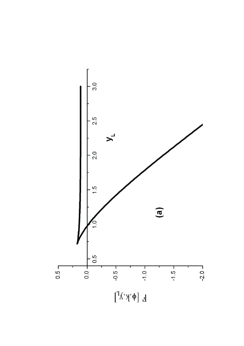
Figure 2: ${\cal F}[\phi,k,L]$ vs. $L$: NEP evaluated at the stationary solutions $\phi_{0}(y)$, $\phi_{1}(y)$ and $\phi_{u}(y)$. Here $k=3$, $D=1.$, and $\phi_{c}/\phi_{h}=0.193$.

It is important to note that, since the NEP for the unstable solution $\phi_{u}$ is always positive and, for the stable nonhomogeneous structure $\phi_{1}$, ${\cal F}<0$ for $L$ large enough, and ${\cal F}>0$ for small values of $L$, the NEP for this structure vanishes for an intermediate value $L=L^{*}$ of the system size. At that point, the stable nonhomogeneous structure $\phi_{1}(y)$ and the trivial solution $\phi_{0}(y)$ exchange their relative stability.

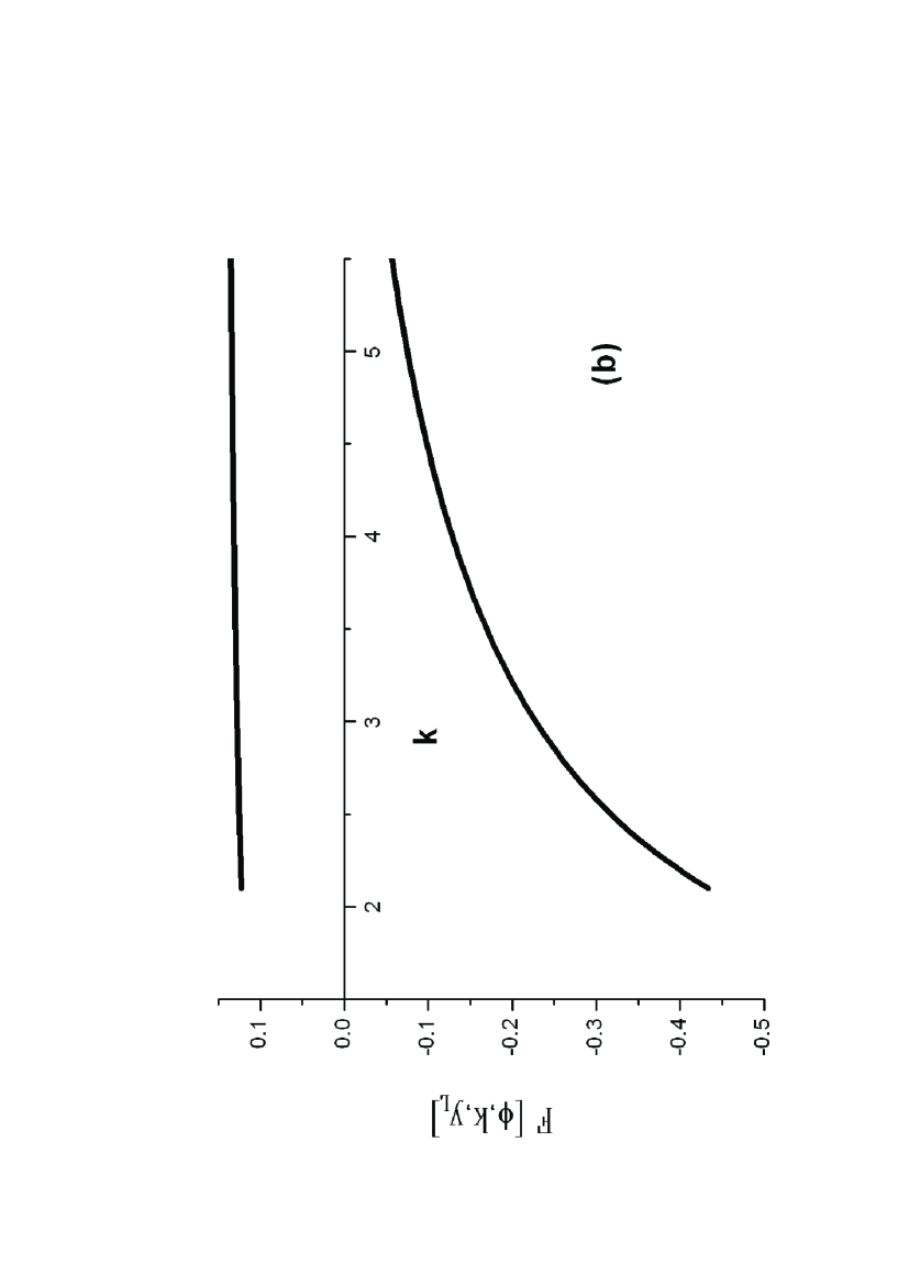
Figure 3: ${\cal F}[\phi,k,L]$ vs. $k$: NEP evaluated at the stationary solutions $\phi_{0}(y)$, $\phi_{1}(y)$ and $\phi_{u}(y)$. Here $L=1.2$, $D=1.$, and $\phi_{c}/\phi_{h}=0.193$.

For completeness and latter use, in Fig. 3 we show ${\cal F}[\phi,k,L]$ but now as a function of $k$, for a fixed value of $L$ and the same value of $z$. Here we see that the initial large difference between the NEP for the states $\phi_{u}(y)$ and $\phi_{1}(y)$ reduces for increasing $k$ until, for $k\to\infty$, the values for Dirichlet b.c. are asymptotically reached.

II.2 System Size Stochastic Resonance

In order to account for the effect of fluctuations, we include in the time–evolution equation of our model (Eq.(1)) a fluctuation term, that we model as an additive noise source extend3b ; nsp , yielding a stochastic partial differential equation for the random field $\phi(y,t)$

$$\frac{\partial}{\partial t}\phi(y,t)=D\,\frac{\partial^{2}}{\partial y^{2}}\phi-\phi+\phi_{h}\,\theta(\phi-\phi_{c})+\xi(y,t).$$ (7)

We make the simplest assumptions about the fluctuation term $\xi(y,t)$, i.e. that it is a Gaussian white noise with zero mean and a correlation function given by

$$\langle\xi(y,t)\,\xi(y^{\prime},t^{\prime})\rangle=2~{}\gamma~{}\delta(t-t^{\prime})~{}\delta(y-y^{\prime}),$$

where $\gamma$ denotes the noise strength.

As was discussed in extend2 ; extend2b ; extend3a ; extend3b , using known results for activation processes in multidimensional systems HG , we can estimate the activation rate according to the following Kramers’ like result for $\langle\tau\rangle$, the first-passage-time for the transitions between attractors,

$$\langle\tau_{i}\rangle=\tau_{0}\,\exp\left\{\frac{\Delta{\cal F}^{i}[\phi,k]}{\gamma}\right\},$$ (8)

where $\Delta{\cal F}^{i}[\phi,k,L]={\cal F}[\phi_{u}(y),k,L]-{\cal F}[\phi_{i}(y),k,L]$ ($i=0,1$). The pre-factor $\tau_{0}$ is usually determined by the curvature of ${\cal F}[\phi,k,L]$ at its extreme and typically is, in one hand, several orders of magnitude smaller than the average time $\langle\tau\rangle$, while on the other –around the bistable point– does not change significatively when varying the system’s parameters. Hence, in order to simplify the analysis, we assume here that $\tau_{0}$ is constant and scale it out of our results. The behavior of $\langle\tau\rangle$ as a function of the different parameters ($k$, $\phi_{c}/\phi_{h}$) was shown in extend2 ; extend2b ; I0 .

As was done in extend2 , we assume now that the system is (adiabatically) subject to an external harmonic variation of the parameter $\phi_{c}$: $\phi_{c}(t)=\phi_{c}^{*}+\delta\phi_{c}\cos(\omega t)$ extend2b ; extend3b , and exploit the “two-state approximation” RMP as in extend2b ; extend3a ; extend3b . Such an approximation basically consist in reducing the whole dynamics on the bistable potential landscape to a one where the transitions occurs between two states: the ones associated to the bottom of each well, while the dynamics is contained only in the transition rates. For all details on the general two-state approximation we refer to extend3a .

Up to first-order in the amplitude $\delta\phi_{c}$ (assumed to be small in order to have a sub-threshold periodic input) the transition rates $W_{i}$ adopt the form

$$W_{i}=\tau_{0}^{-1}\exp\left\{-\frac{\Delta{\cal F}^{i}[\phi,k,L,t]}{\gamma}\right\}$$ (9)

where

$$\Delta{\cal F}^{i}[\phi,k,L,t]=\Delta{\cal F}^{i}[\phi,k,L]+\delta\phi_{c}\Bigl{(}\frac{\partial\Delta{\cal F}^{i}[\phi,k,L]}{\partial\phi_{c}}\Bigr{)}_{\phi_{c}=\phi_{c}^{*}}\cos(\omega t).$$ (10)

This yields for the transition probabilities

$$W_{i}\simeq\frac{1}{2}\Bigl{(}\mu_{i}\mp\alpha_{i}\frac{\delta\phi_{c}}{\gamma}\cos(\omega t)\Bigr{)},$$ (11)

where

$$\mu_{i}\approx\exp\left\{-\frac{\Delta{\cal F}^{i}[\phi,k,L]}{\gamma}\right\}$$

and

$$\alpha_{i}\approx\pm\mu_{i}\left(\frac{d\Delta{\cal F}^{i}}{d\phi_{c}}\right)_{\phi_{c}^{*}},$$

($i=1,2$). Using Eq. (6), it is clear that $\frac{d\Delta{\cal F}^{i}}{d\phi_{c}}|_{\phi_{c}^{*}}$ can be obtained analytically.

These results allows us to calculate the autocorrelation function, the power spectrum density and finally the SNR, that we indicate by $R$. The details of the calculation were shown in extend3a and will not be repeated here. For $R$, and up to the relevant (second) order in the signal amplitude $\delta\phi_{c}$, we obtain extend3a

$$R=\,\frac{\pi}{4\,\mu_{1}\,\mu_{2}}\frac{(\alpha_{2}\,\mu_{1}+\alpha_{1}\,\mu_{2})^{2}}{\mu_{1}+\mu_{2}}.$$ (12)

Due to the form of $\alpha_{i}$, we can reduce the previous expression to

$$R=\,\frac{\pi}{4\,\gamma^{2}}\frac{\mu_{1}\,\mu_{2}}{\mu_{1}+\mu_{2}}\Phi,$$ (13)

where

$$\Phi=\left[\int_{-L/2}^{L/2}\phi_{h}\,\theta(\phi_{st}(y)-\phi_{c})\,dy\right]^{2}=\left[2\,\phi_{h}\,y_{c}(L)\right]^{2}.$$ (14)

We have now all the elements required to analyze the problem of SSSR.

Figure 4 shows the typical behavior of SR, but now –in the horizontal axis– the noise intensity is replaced by the the system length $L$, for fixed values of $k$, $\gamma$ (the noise intensity) and the ratio $\phi_{c}/\phi_{h}$ (that in our scaled system is a single parameter). Such a response is the expected one for a system exhibiting SSSR. Within the context of NEP, it results clear that, in this kind of systems, the phenomenon arises due to the breaking of the NEP’s potential symmetry. This means that, as shown in Fig. 2, due to the variation of $L$, both attractors can exchange their relative stability. For a value $L=L^{*}$, both stable structures, the nonhomogeneous $\phi_{1}(y)$ and the trivial $\phi_{0}(y)$, have the same value for the NEP. When $L<L^{*}$, $\phi_{1}(y)$ becomes less stable than $\phi_{0}(y)$, making the transitions from $\phi_{1}(y)$ to $\phi_{0}(y)$ “easier” (the barrier is lower) than in the reverse direction, reducing the system’s response. When $L\sim 0.72$, $\phi_{1}(y)$ and $\phi_{u}(y)$ coalesce and disappear, and the response is strictly zero (within the linear response implicit in the two state approximation). When $L>L^{*}$, $\phi_{1}(y)$ becomes more stable than $\phi_{0}(y)$, making now the transitions from $\phi_{0}(y)$ to $\phi_{1}(y)$ “easier” than in the reverse direction, again reducing the system’s response. Clearly, the system’s response has a maximum when both attractors have the same stability ($L=L^{*}$), and decays when departing from that situation. Hence, for this system and within this framework, SSSR arises as a particular case of the more general discussion done in extend3a .

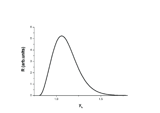
Figure 4: SNR, vs. $L$, for $k=3.$, $\gamma=0.1$, $D=1.$, and $\phi_{c}/\phi_{h}=0.193$.

We can analyze the same problem from an alternative point of view. That is, studying the scaling of the NEP in Eq. (4) with $L$. Due to the similarities of the present problem with the one discussed in Section IV, we stop here the discussion, and left such a kind of analysis to treat that problem.

To conclude this section as well as for completeness, we change the point of view. In Fig. 5 we show the curves of the SNR as a function of $k$, while keeping fixed values of $L$, and $z$. When $k$ is not too large, indicating a high degree of reflectiveness at the boundary (that is, a reduced exchange with the environment), we see that the SNR changes for $k$ varying from low to larger values, showing a broad resonance like curve. Remember that a large value of $k$ indicates that the system boundaries become absorbent. Such a broadening of the resonance indicates the robustness of the systems’ response when varying $k$, a parameter that somehow indicates a degree of coupling with the environment. However, according to the previous argument –about the breaking of NEP’s symmetry– from the behavior in Fig. 3 this is again the expected result.

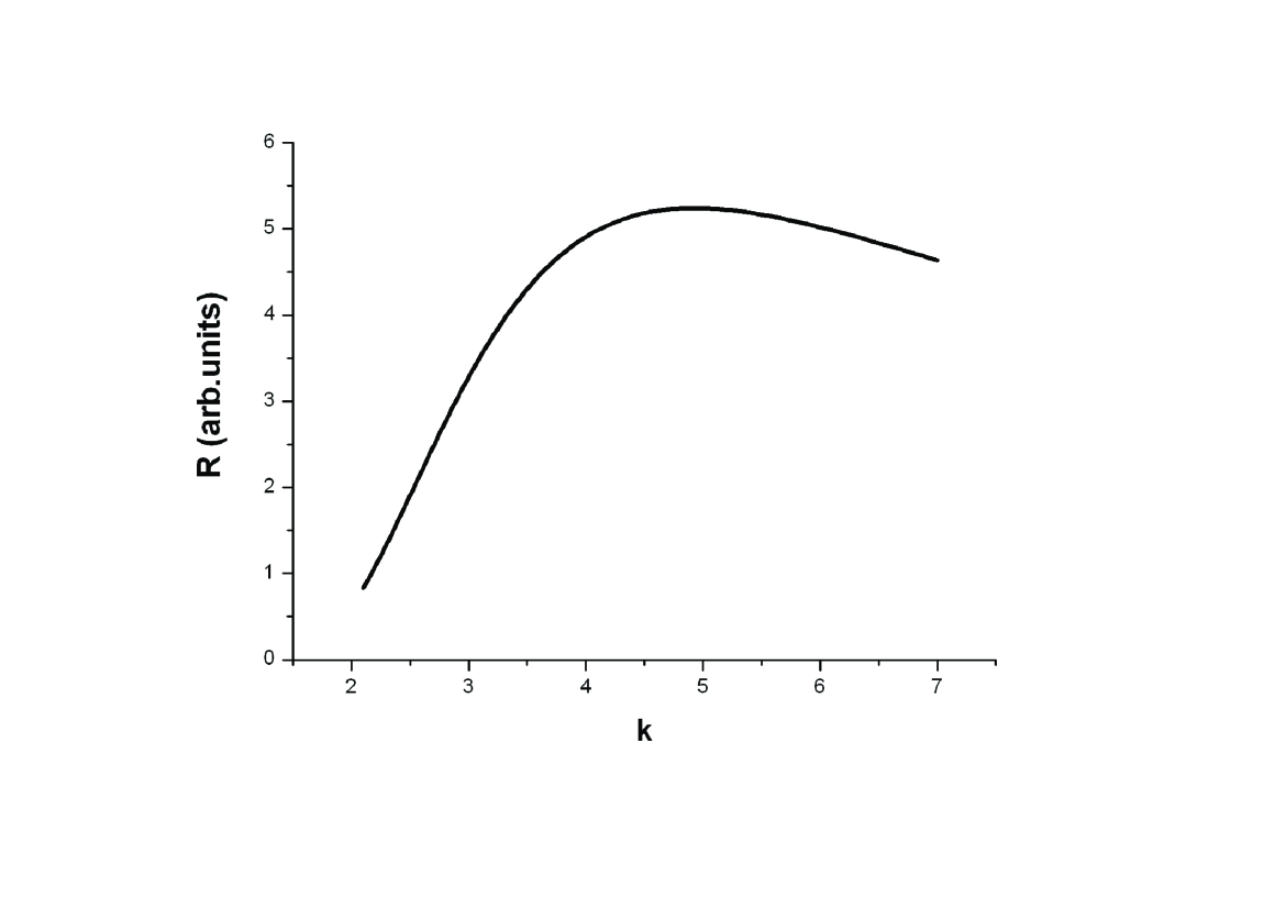
Figure 5: SNR, vs. $k$ for $L=1.2$, $\gamma=0.1$, $D=1.$, and $\phi_{c}/\phi_{h}=0.193$.

III The Global Coupling Model

In this section we consider one of the models discussed in SSSR4 from the point of view of the NEP approach. The model we refer to is described by a set of (globally) coupled nonlinear bistable oscillators

$$\dot{x}_{j} = x_{j}-x_{j}^{3}+\frac{\varepsilon}{N}\sum_{k=1}^{N}(x_{k}-x_{j})+\sqrt{2\,\gamma}\,\xi_{j}(t)+f_{j}(t),$$

$$\dot{x}_{j} = -\frac{\partial}{\partial\,x_{j}}U(\{x\},t)+\sqrt{2\,\gamma}\,\xi_{j}(t),$$ (15)

with $f_{j}(t)=A\cos(\omega t)$, $\{x\}=(x_{1},x_{2},..,x_{N})$, $\xi_{j}(t)$ are Gaussian noises with zero mean and $\langle\xi_{j}(t)\xi_{l}(t^{\prime})\rangle=\delta_{jl}\,\delta(t-t^{\prime})$, and where we have defined

$$U(\{x\},t) = U_{0}(\{x\})-A\cos(\omega t)\sum_{j=1}^{N}x_{j}$$ (16)

$$= \sum_{j=1}^{N}\left(\frac{x_{j}^{4}}{4}-\frac{x_{j}^{2}}{2}\right)+\frac{\varepsilon}{2\,N}\sum_{j=1}^{N}\sum_{k=1}^{N}(x_{k}-x_{j})^{2}-A\cos(\omega t)\sum_{j=1}^{N}x_{j}$$

$$= \sum_{j=1}^{N}u_{0}(x_{j})+\frac{\varepsilon}{2\,N}\sum_{j=1}^{N}\sum_{k=1}^{N}(x_{k}-x_{j})^{2}-A\cos(\omega t)\sum_{j=1}^{N}x_{j}.$$

Due to the structure of Eq. (III) it is clear that $U_{0}(\{x\})$, the potential function in Eqs. (III,16), is the discrete form of the NEP for this problem. For $A=0$ the stationary distribution of the multidimensional Fokker-Planck equation associated to Eq. (III) results

$$P_{stat}(\{x\})\approx\exp\left(-\frac{U_{0}(\{x\})}{\gamma}\right).$$ (17)

This potential has two attractors corresponding to $x_{1}=x_{2}=...=x_{N}=\pm 1$, and a barrier separating them at $x_{1}=x_{2}=...=x_{N}=0$.

Now, exploiting the same scheme as before but, as both attractors have the same “energy”, reduced to the symmetric case, we get for the SNR

$$R\approx\exp\left(-\frac{\triangle U_{0}(\{x\})}{\gamma}\right)\approx\frac{N}{\gamma}\,\exp\left(-\frac{N\,\triangle u_{0}(X)}{\gamma}\right),$$ (18)

where $X$ is a kind of “collective coordinate” (the one evolving along the trajectory joining both attractors, that pass though the saddle, and that can be approximately interpreted as $X\approx\frac{1}{N}\sum_{j=1}^{N}x_{j}$. However, we need the evaluation at only two points: $X=0,\pm 1$), and

$$\triangle u_{0}(X)=u_{0}(X=\pm 1)-u_{0}(X=0).$$

Such a SNR clearly shows similar SSSR characteristics as those described in SSSR4 . In this situation the NEP’s symmetry is retained when varying $N$, while the wells are deepened (or the barrier separating them is enhanced). However, if we scaled out $N$, we find a constant “effective” potential ($u_{0}(X)$), while the system shows an effective scaling of the noise with $N$. In this case we could speak of a noise scaled SSSR, in contrast to the previous case that could be called a NEP symmetry breaking SSSR.

In order to deepen our understanding of this case, let us analyze a continuous model, that is tightly connected with the previous discrete one. Consider a field $\psi(y,t)$, that behaves according to the following functional equation

$$\frac{\partial}{\partial\,t}\psi(y,t) = \psi(y,t)-\psi(y,t)^{3}+\varepsilon\int_{\Omega}(\psi(y^{\prime},t)-\psi(y,t))\,dy^{\prime}+\xi(y,t)+f(t),$$ (19)

$$= -\frac{\delta}{\delta\,\psi(y,t)}U(\psi(y,t))+\xi(y,t),$$

with $f(t)=A\cos(\omega t)$, while for the noise we assume that, as before, it is white and Gaussian with $\langle\xi(y,t)\rangle=0$, and the correlation

$$\langle\xi(y,t)\xi(y^{\prime},t^{\prime})\rangle=2\,\gamma\,\delta(y-y^{\prime})\delta(t-t^{\prime}).$$

$\Omega$ indicates the integration range, and $\frac{\delta}{\delta\,\psi(y,t)}$ is a functional derivative. We consider a finite system in the interval $y\in[-L/2,L/2]$, and assume Neumann boundary conditions. The form of the potential $U(\psi(y,t),t)$ results

$$U(\psi(y,t)) = U_{0}(\psi(y,t))-F(\psi(y,t))$$

$$= \int_{\Omega}\,dy\,u_{0}(\psi(y,t))+\frac{\varepsilon}{2}\,\int_{\Omega}\,dy\,\int_{\Omega}\,dy^{\prime}\,\left(\psi(y^{\prime},t)-\psi(y,t)\right)^{2}-F(\psi(y,t)),$$

where

$$u_{0}(\psi(y,t))=\left(\frac{\psi(y,t)^{4}}{4}-\frac{\psi(y,t)^{2}}{2}\right),$$

and

$$F(\psi(y,t))=A\cos(\omega t)\int_{\Omega}\psi(y,t)\,dy.$$

This potential is clearly similar to the one discussed in extend2b , but with the local (diffusive) coupling being zero, and the nonlocal contribution becoming “global”. For $A=0$ the stationary distribution of the multidimensional Fokker-Planck equation associated to Eq. (19) results

$$P_{stat}(\psi_{stat}(y))\approx\exp\left(-\frac{U_{0}(\psi_{stat}(y))}{\gamma}\right),$$ (21)

with $\gamma$ the noise intensity. This potential has two attractors corresponding to the constant fields $\psi_{stat}(y)=\pm 1$, and a barrier separating them at $\psi_{stat}(y)=0$.

Hence, exploiting the same scheme as in the previous section, but reduced to the symmetric case as both attractors have the same “energy”, we get for the SNR

$$R\approx\exp\left(-\frac{\triangle U_{0}(\psi_{stat}(y))}{\gamma}\right)\approx\frac{L}{\gamma}\,\exp\left(-\frac{L\,\triangle u_{0}(\psi_{stat}(y))}{\gamma}\right).$$ (22)

where

$$\triangle u_{0}(\psi_{stat}(y))=u_{0}(\psi_{stat}(y)=\pm 1)-u_{0}(\psi_{stat}(y)=0).$$

This SNR clearly shows the same SSSR characteristics as those described for the discrete case, where the role of $N$ (number of elements) is now played by $L$ (size of the system).

Note that Eq. (19) corresponds to the continuous limit of Eq. (III) and the result for the discrete case (Eq. (18)) is recovered in Eq. (22) for the normalized noise intensity $\gamma_{dc}=\gamma/\Delta x$ (with $\gamma_{dc}$ the noise intensity for the discrete case), and $L=N\Delta x.$

To conclude this section, we refer to another case discussed in SSSR4 , the one corresponding to the Ising model. Such a case has many similarities with the case of the set of coupled nonlinear bistable oscillators discussed above. It can be described in a similar way to the case above. That means we could also find an effective potential playing the role of the NEP, having two attractors (corresponding to all spins up or all down), a barrier corresponding to a mixed state, whose high depends linearly with $N$ (the number of spins). The final result will be similar to the one in Eq. (18) above.

IV Multiplicative Noise Case

IV.1 Brief Review of the Model

The basic model to be considered in this section is the same one studied in WeNew , and consist of the following ensemble of nonlinear coupled oscillators, described in terms of a continuous field

$$\frac{\partial}{\partial t}\phi(y,t)=\frac{\partial}{\partial y}\left(D(\phi)\,\frac{\partial}{\partial y}\phi\right)+f(\phi)+\frac{1}{\sqrt{D(\phi)}}\,\xi(y,t).$$ (23)

Here $\xi(y,t)$ is again a Gaussian white noise with zero mean and correlation $\langle\xi(y,t)\xi(y^{\prime},t^{\prime})\rangle=2\gamma\delta(y-y^{\prime})\delta(t-t^{\prime})$, being $\gamma$ the noise intensity. $D(\phi)$ is a field-dependent diffusivity and the coefficient of the noise term guarantee that fluctuation-dissipation relation is fulfilled kitara . The nonlinearity $f(\phi)$ which drives the dynamics in absence of noise is monostable, and we adopt a density dependent diffusion coefficient to generate a noise-induced bistable dynamics. In particular, we use

$$D(\phi)=\frac{D_{0}}{1+h\phi^{2}},$$ (24)

and

$$f(\phi)=-\phi^{3}+b\,\phi,$$ (25)

being $D_{0}$, $h$ and $b$ positive constants. We will consider a finite system, limited to ($-L/2\leq x\leq L/2$), and assume Dirichlet boundary conditions $\phi(\pm L/2)=0$.

As we are considering the Stratonovich interpretation, the stationary solution of the probability $P_{st}(\phi)$ of the stochastic field $\phi(x,t)$ given by Eq. (23) can be written ibanyes in terms of an effective potential

$$P_{st}(\phi)\sim\exp(-V_{eff}/\gamma),$$ (26)

with

$$V_{eff}[\phi] = \int_{-L/2}^{L/2}dy\bigg{\{}\frac{1}{2}\left(D(\phi)\frac{\partial}{\partial y}\phi\right)^{2}-U(\phi)-\lambda\,\ln D(\phi)\bigg{\}},$$ (27)

(where $U(\phi)=\int_{0}^{\phi}D(\phi^{\prime})f(\phi^{\prime})\,d\phi^{\prime}$). Here $\lambda$ is a renormalized parameter, related to $\gamma$ by $\lambda=\gamma/2\,\Delta y$ in a square discrete lattice, where $\Delta y$ is the lattice parameter ibanyes . The extremes of $V_{eff}$— stationary noise-induced structures of the effective dynamics— can be computed from

$$\frac{\partial}{\partial y}\left(D(\phi)\,\frac{\partial}{\partial y}\phi\right)+F_{eff}(\phi)=0$$ (28)

with an effective nonlinearity

$$F_{eff}(\phi)=f(\phi)+\lambda\frac{1}{D(\phi)^{2}}\frac{d}{d\phi}D(\phi)=\phi\,(\phi-\phi_{1})\,(\phi_{2}-\phi),$$ (29)

where $\phi_{1,2}$ depend on parameters, in particular on the renormalized noise intensity $\lambda$. (We have found one trivial homogeneous structure $\phi=0$ and two nonhomogeneous patterns, the unstable (saddle) $\phi_{u}$ and the stable one $\phi_{s}$ (see Ref. WeNew )).

We note that in the deterministic problem we have a monostable foot1 reaction term ($\lambda=0$). As we increase the noise intensity, due to the noise effects, we have an effective nonlinear term $F_{eff}$ that results to be bistable (in the interval $0<\lambda<D_{0}/(2h)$) and finally monostable for $\lambda>D_{0}/(2h)$ (reentrance effect). We also remark that $\phi=0$ is always a root of $F_{eff}$ (see Fig. 6), and it is an extremum of $V_{eff}[\phi]$ for all values of $\lambda$. In what follows we will call this structure $\phi_{0}$. As a final remark, the situation here is that the same noise that induces the patterns and the bistability is the one inducing the transitions among them and the SR phenomenon.

Figure 6: Form of the nonlinearities for the deterministic case ($\lambda=0$), bistable case ($\lambda=0.8$) and a monostable case ($\lambda=1.2$) in the reentrance region. The vertical scale was changed in the deterministic case in order to clarify the figure. Note that $\phi=0$ remains as a root in all cases. The parameters used are: $D_{0}=1$, $h=1/2$ and $b=2$.

IV.2 System Size Stochastic Resonance

To analytically describe the stochastic resonance, again we resort to use the two state approach in the adiabatic limit RMP . As indicated before, all details about the procedure and the evaluation of the SNR could be found in extend3a . The system is now subject to a time periodic subthreshold signal $b=b_{0}+S(t)$ where $S(t)=\Delta b\,\sin(\omega_{0}t)$. Up to first-order in the small amplitude $\Delta b$ the transition rates $W_{i}$ take the form

$$W_{1}(t) = \mu_{1}-\alpha_{1}\,\Delta b\,\sin(\omega_{0}\,t),$$

$$W_{2}(t) = \mu_{2}+\alpha_{2}\,\Delta b\,\sin(\omega_{0}\,t),$$ (30)

where the constants $\mu_{1,2}$ and $\alpha_{1,2}$ are obtained from the Kramers-like formula for the transition rates HG

$$W_{\phi_{i}\rightarrow\phi_{j}}=\frac{\beta_{+}}{2\pi}\,\left[\frac{\det\,V_{eff}(\phi_{i})}{|\det\,V_{eff}(\phi_{s})|}\right]^{1/2}\,\exp[-(V_{eff}(\phi_{i})-V_{eff}(\phi_{s}))/\gamma].$$ (31)

Here $\beta_{+}$ is the unstable eigenvalue of the deterministic flux at the relevant saddle point ($\phi_{s})$ and

$$\mu_{1,2} = W_{1,2}|_{S(t)=0},$$

$$\alpha_{1,2} = \mp\frac{dW_{1,2}}{dt}|_{S(t)=0}.$$ (32)

We note in passing that, due to the system’s sensitivity to small variations in the parameters, and at variance with the case studied in Section II, here we require the evaluation of the pre-factor in Eq. (31).

As before, these results allows us to calculate the autocorrelation function, the power spectrum and finally the SNR (indicated by $R$). For $R$, up to the relevant (second) order in the signal amplitude $\Delta b$, similarly to Eq. (12) and (13) we obtain

$$R=\frac{\pi}{4\,\mu_{1}\,\mu_{2}}\frac{(\alpha_{2}\,\mu_{1}+\alpha_{1}\,\mu_{2})^{2}}{\mu_{1}+\mu_{2}}=\frac{\pi}{4\gamma^{2}}\,\frac{\mu_{1}\,\mu_{2}}{\mu_{1}+\mu_{2}}\,\Phi,$$ (33)

where now

$$\Phi=\int_{-L/2}^{L/2}dy\,\int_{\phi_{0}}^{\phi_{s}(y)}\,D(\phi^{\prime})\,\phi^{\prime 2}\,d\phi^{\prime}$$ (34)

gives a simultaneous measure of the spatial coupling (through $D(\phi)$) and the system size extension (through $\int dy$). In our previous work WeNew we have found that the dependence of the SNR as a function of $\lambda$ is maximum at the symmetric situation $\lambda=\lambda_{c}=0.8$, where both stable structures ($\phi_{0}$ and $\phi_{s}$) have the same stability ($V_{eff}[\phi_{0}]=V_{eff}[\phi_{s}]$).

To analyze the system size dependence of the SR, we fix the renormalized noise intensity ($\lambda=\lambda_{c}=0.8$) and the parameters $D_{0}=1$, $b=2$ and $h=1/2$; only change the length $L$ (with fixed lattice parameter $\Delta x$).

It is worth here remarking that in SSSR4 what is varied is the length of the lattice, while the noise intensity, the coupling, etc, are kept constant. In the present case, due to the characteristics of the model, we have that as $L$ is varied, the fields change inducing the change of the diffusive coupling, making a strong difference with the case in SSSR4 .

At this point we can just analyze the dependence of the SNR with $L$ as was done in Section II. However, as was indicated near the end of that section, we use an alternative for of analysis, looking at the scaling of the potential with $L$. We consider the following transformations

• $y\to x=\frac{y}{L}$,

• $D_{o}\to D_{1}=\frac{D_{o}}{L}$,

• $D(\phi)=\frac{D_{o}}{1+h\,\phi^{2}}\to D_{1}(\phi)=\frac{D_{1}}{1+h\,\phi^{2}}$,

the effective potential (Eq. (27) could be written as

$$V_{eff}[\phi]=L\,\int_{-1/2}^{1/2}dx\bigg{\{}-U(\phi)+\frac{1}{2}\left[\frac{D(\phi)}{L}\frac{\partial}{\partial x}\phi\right]^{2}\bigg{\}}-\lambda\,L\int_{-1/2}^{1/2}dx\ln D(\phi),$$ (35)

that finally yields (using the previous definition $D(\phi)/L=D_{1}(\phi)$)

$$V_{eff}[\phi]/L=V_{sc}(L)=\,\int_{-1/2}^{1/2}dx\bigg{\{}-U(\phi)+\frac{1}{2}\left[D_{1}(\phi)\frac{\partial}{\partial x}\phi\right]^{2}-\lambda\ln D_{1}(\phi)\bigg{\}}-\lambda\ln L.$$ (36)

Here it becomes apparent that this scaling yields a logarithmic length contribution to the scaled potential.

The stationary solution $P_{st}(\phi)$ (see Eq. 26) of the stochastic field $\phi(y,t)$ can be written

$$P_{st}(\phi)\sim\exp(-V_{sc}(L)/\gamma_{x}(L)),$$ (37)

with $\gamma_{x}(L)=\gamma/L$.

We can also consider the scaling of the spatial factor $\Phi$ (see Eq. (34)). It results

$$\Phi=L\,\int_{-1/2}^{1/2}dx\,\int_{\phi_{0}}^{\phi_{s}(x)}D(\phi^{\prime})\,\phi^{\prime 2}\,d\phi=L\,\frac{D_{0}}{h}\int_{-1/2}^{1/2}dx\,\left\{\phi_{s}(x)-\frac{\arctan(\sqrt{h}\,\phi_{s}(x))}{\sqrt{h}}\right\}.$$ (38)

Hence, we have the dependence of the NEP as well as transitions rates (Eq. (31)) and finally of the SNR (Eq. (33)), on the system length (or the number of coupled elements for discrete systems). To illustrate this, in Fig. 7 we show $V(\phi_{eff})$ as a function of $L$. The behavior shown in this figure is analogous to the one observed in Fig. 2. Hence, we can anticipate the existence SSSR in this system.

We see that for small $L$, small size effects increase the NEP values of the nonhomogeneous structures, and the uniform state results to be the most stable one. It becomes metastable at $L_{c}$, and nonuniform patterns are the globally stable attractors for larger values of $L$. The rate transitions also reflect this fact (they are decreasing functions of $L$). However, we expect that $\Phi$— which depends on the system size—, increases with $L$, and due to the interplay of the rates and the behavior of $\Phi$, a SSSR can be expected. Such a behavior becomes apparent in Fig. 8.

Figure 7: Nonequilibrium potential $V_{eff}[\phi_{st}]$ evaluated in the stationary structures as a function of the system size $L$. Curves correspond to: (1) stable ($\phi_{s}$), (2) homogeneous ($\phi_{0}$) and (3) unstable ($\phi_{u}$) patterns. Note the global stabilization of the nontrivial stable pattern for high values of $L$.

Figure 8: Signal-to-noise ratio vs. $L$. As indicated in the text, we fixed $D_{o}=1$, $h=0.5$, $b=2$, and $\lambda=\lambda_{c}=0.8$.

We can make the following interpretation in terms of $V_{sc}(L)$, the “effective” NEP (the scaled form of the NEP, Eq. (36)), and the the scaling of the noise intensity. In Fig. 9 we depict the form of $V_{sc}(L)$ as function of $L$. It is clear that, even though it is weak, the dependance of $V_{sc}(L)$ with $L$ still shows the change in the relative stability of the attractors, while we have the scaling of the noise intensity with $L$. Hence, we can argue that there is a kind of “effective entanglement” between the symmetry breaking and the noise scaling.

Figure 9: $V_{sc}(L)/L$ evaluated on the stationary structures as a function of the system size $L$. Curves correspond to: (1) stable ($\phi_{s}$), (2) homogeneous ($\phi_{0}$) and (3) unstable ($\phi_{u}$) patterns. These corresponds to the same curves as in Fig. 7.

V Conclusions

The study of SR in extended or coupled systems, motivated by both, some experimental results and the growing technological interest, has recently attracted considerable attention extend1 ; otros ; extend2 ; extend2b ; extend3a ; extend3b ; extend3c . In previous papers extend2 ; extend2b ; extend3a ; extend3b ; extend3c we have studied the SR phenomenon for the transition between two different patterns, exploiting the concept of nonequilibrium potential GR ; I0 ; WeNew .

Recent works SSSR1 ; SSSR2 ; SSSR3 have shown that several systems presents intrinsic SR-like phenomena as the number of units, or the size of the system is varied. This phenomenon, called system size stochastic resonance, has also been found in a set of globally coupled units described by a $\phi^{4}$ theory SSSR4 , and even shown to arise in opinion formation models SSSR5 . Such SSSR phenomenon occurs in extended systems, hence it was clearly of great interest to have a description of this phenomenon within the NEP framework.

Here, we have discussed in detail two of the cases analyzed in SSSR6 and presented a third, interesting one, that corresponds to the study of the system size dependence of SR in the same system studied in WeNew .

A relevant aspect that arose from these studies is that there is a kind of entrainment between the symmetry breaking of the NEP as described in SSSR6 , together with a scaling of noise intensity with system size as in SSSR4 .

In the first case we focused on a simple reaction-diffusion model with a known form of the NEP WW ; RL , and –as in all three cases– considering the adiabatic limit and exploiting the two-state approximation, we were able to clearly quantify the system size dependence of the SNR. We have shown that in this case, SSSR is associated to a NEP’s symmetry breaking. For the second case we analyzed the model of globally coupled nonlinear oscillators discussed in SSSR4 , and have shown that it can also be described within the NEP framework, but now SSSR arises through an “effective” scaling of the noise intensity with the system size. For the third studied case, we have obtained the exact form of the noise-induced patterns (both the stable and unstable ones) as well as the analytical expression of the NEP. The interplay of the transition rates, that are essentially decreasing functions of $L$, and the behavior of $\Phi$, that increases with $L$, explain the existence of a maximum in the SNR for a specific length of the system and a fixed noise intensity. What arose here, through an alternative form of analysis, is that there is a kind of entrainment between the symmetry breaking of the NEP as described in SSSR6 , together with a scaling of noise intensity with the system size as in SSSR4 .

The results found in this work clearly show that the “nonequilibrium potential” (even if not known in detail, see for instance quasi ) offers a very useful framework to analyze a wide spectrum of characteristics associated to SR in spatially extended or coupled systems. Within this framework the phenomenon of SSSR looks, as other aspects of SR in extended systems extend3a , as a natural consequence of a breaking of the symmetry of the NEP or to an effective scaling of the noise intensity as in SSSR4 , or could be interpreted as an entrainment between the two aspects.

In addition, in the first studied case, we have seen a new form of resonant behavior through the variation of the coupling with the surroundings. In such a case the system’s response to an external signal becomes more robust, that is less sensitive to the precise value of the albedo parameter. This fact opens new possibilities for analyzing and interpreting the behavior of some biological systems neubio .

As a final comment, the main difference between the first and third cases when compared with the second one, is that in the two former cases we have local interactions with albedo b.c. (covering the range from Neumann to Dirichlet b.c.), while the latter has a non local coupling together with boundary conditions that could be assumed as Neumann. From our results, it is possible to argue that the effective scaling of the noise that arises in the second case comes from the non local interaction, and not from the b.c. To make this aspect more obvious, we plan to study, within the present framework, the competence between local and non-local spatial couplings extend2b ; extend3b , that arise in some multi-component models. Also, the consideration of more general systems with several components will allow us to analyze the system size dependence of SR between patterns in general activator-inhibitor-like systems. All these aspects will be the subject of further work.

- (1) Member of CONICET, Argentine.
- (2) L. Gammaitoni, P. Hänggi, P. Jung and F. Marchesoni, Rev. Mod. Phys. 70, 223 (1998).
- (3) J. K. Douglas et al., Nature 365, 337 (1993); J. J. Collins et al., Nature 376, 236 (1995); S. M. Bezrukov and I. Vodyanoy, Nature 378, 362 (1995).
- (4) A. Guderian, G. Dechert, K. Zeyer and F. Schneider; J. Phys. Chem. 100, 4437 (1996); A. Förster, M. Merget and F. Schneider; J. Phys. Chem. 100, 4442 (1996); W. Hohmann, J. Müller and F. W. Schneider; J. Phys. Chem. 100, 5388 (1996).
- (5) J. F. Lindner, B. K. Meadows, W. L. Ditto, M. E. Inchiosa and A. Bulsara, Phys. Rev. E 53, 2081 (1996).
- (6) A. Bulsara and G. Schmera, Phys. Rev. E 47, 3734 (1993); P. Jung, U. Behn, E. Pantazelou and F. Moss, Phys. Rev. A 46, R1709 (1992); Jung and Mayer-Kress, Phys. Rev. Lett. 74, 208 (1995); J. F. Lindner, B. K. Meadows, W. L. Ditto, M. E. Inchiosa and A. Bulsara, Phys. Rev. Lett. 75, 3 (1995); F. Marchesoni, L. Gammaitoni and A. Bulsara, Phys. Rev. Lett. 76, 2609 (1996).
- (7) H. S. Wio, Phys. Rev. E 54, R3045 (1996); H. S. Wio and F. Castelpoggi, Proc. Conf. UPoN’96, C. R. Doering, L. B. Kiss and M. Schlesinger Eds. World Scientific, Singapore; F. Castelpoggi and H. S. Wio, Europhys. Lett. 38, 91 (1997).
- (8) F. Castelpoggi and H. S. Wio, Phys. Rev. E 57, 5112 (1998).
- (9) S. Bouzat and H. S. Wio, Phys. Rev. E 59, 5142 (1999).
- (10) H. S. Wio, S. Bouzat and B. von Haeften, in Proc. 21st IUPAP Int.Conf.on Statistical Physics, STATPHYS21, A.Robledo and M. Barbosa (Eds.), Physica A 306C 140-156 (2002).
- (11) C. J. Tessone, H. S. Wio and P. Hänggi, Phys. Rev. E 62, 4623 (2000).
- (12) M. A. Fuentes, R. Toral and H. S. Wio, Physica A 295 114 (2001).
- (13) B. von Haeften, R. Deza and H. S. Wio, Phys. Rev. Lett. 84, 404 (2000).
- (14) R. Graham and T. Tel, in Instabilities and Non-equilibrium Structures III, E. Tirapegui and W. Zeller, eds. (Kluwert, 1991); H. S. Wio, in 4th. Granada Seminar in Computational Physics, Eds. P. Garrido and J. Marro (Springer-Verlag, Berlin, 1997), pg.135.
- (15) G. Izús et al, Phys. Rev. E 52, 129 (1995); G. Izús et al, Int. J. Mod. Physics B 10, 1273 (1996); D. H. Zanette, H. S. Wio and R. Deza, Phys. Rev. E 53, 353 (1996); F. Castelpoggi, H. S. Wio and D. H. Zanette, Int. J. Mod. Phys. B 11, 1717 (1997).
- (16) B. von Haeften, et al., Phys. Rev. E 69, 021107 (2004); B. von Haeften, et al., in Noise in Complex Systems and Stochastic Dynamics, Z. Gingl, J.M. Sancho, L. Schimansky-Geier and J. Kerstez (Eds.), Proc. SPIE 5471, 258-265 (2004).
- (17) G. Schmid, I. Goychuk, P. Hänggi, Europhys. Lett. 56, 22 (2001); G. Schmid, I. Goychuk, P. Hänggi, Phys. Biol. 1, 61 (2004).
- (18) P. Jung, J.W. Shuai, Europhys. Lett. 56, 29 (2001); J.W. Shuai, P. Jung, Phys. Rev. Lett. 88, 068102 (2003).
- (19) R. Toral, C. Mirasso, J. Gunton, Europhys. Lett. 61, 162 (2003).
- (20) A. Pikovsky, A. Zaikin, M.A. de la Casa, Phys. Rev. Lett. 88, 050601 (2002).
- (21) C. J. Tessone, R. Toral, Physica A (in press), cond-mat/0409620.
- (22) H.S. Wio, System Size Stochastic Resonance from the Viewpoint of the Nonequilibrium Potential, submitted to Phys. Rev. Lett., cond-mat/0410464.
- (23) H. S. Wio, An Introduction to Stochastic Processes and Nonequilibrium Statistical Physics (World Scientific, 1994), chp.5; A.S.Mikhailov, Foundations of Synergetics I, (Springer-Verlag, 1990).
- (24) W.J. Skocpol, M.R. Beasley, M. Tinkham, J. Appl. Phys. 45, 4054 (1974); B. Ross, J.D. Lister, Phys. Rev. A 15, 1246 (1977); D. Bedeaux, P. Mazur, Physica A 105, 1 (1981).
- (25) C.L. Schat and H.S. Wio, Physica A 180, 295 (1992).
- (26) J. García-Ojalvo and J. M. Sancho, Noise in Spatially Extended Systems (Springer-Verlag, New York, 1999).
- (27) P. Hänggi, P. Talkner, and M. Borkovec, Rev. Mod. Phys. 62, 251 (1990).
- (28) M. Morillo, J. Gomez-Ordoñez and J. M. Casado, Phys. Rev. E 52, 316 (1995).
- (29) K. Kitahara and M. Imada, Suppl. Prog. Theor. Phys. 64, 65(1978).
- (30) M. Ibañes, J. García-Ojalvo, R. Toral, and J. M. Sancho, Phys. Rev. Lett. 87, 020601 (2001).
- (31) Monostable means here that the function derive from a monostable potential.
- (32) H.S. Wio, M.N.Kuperman, F.Castelpoggi, G. Izús, R. Deza; Physica A 257, 275 (1998)
- (33) A. Fulinski, Z. Grzywna, I.R. Mellor, Z. Siwy, and P.N.R. Usherwood, Phys. Rev. E 58, 919, (1998); Sz. Mercik and K. Weron, Phys. Rev. E 63, 051910 (2001); I. Goychuk and P. Hanggi, Phys. Rev. E 69, 021104 (2004).