Charge sensitivity of the Inductive Single-Electron Transistor

Abstract

We calculate the charge sensitivity of a recently demonstrated device where the Josephson inductance of a single Cooper-pair transistor is measured. We find that the intrinsic limit to detector performance is set by oscillator quantum noise. Sensitivity better than $10^{-6}$e$/\sqrt{\mathrm{Hz}}$ is possible with a high $Q$-value $\sim 10^{3}$, or using a SQUID amplifier. The model is compared to experiment, where charge sensitivity $3\times 10^{-5}$e$/\sqrt{\mathrm{Hz}}$ and bandwidth 100 MHz are achieved.

Remarkable quantum operations have been demonstrated in the solid state nakamuraqb ; vion ; hanqb . As exotic quantum measurements known in quantum optics are becoming adopted for electronic circuits qed , sensitive and desirably non-destructive measurement of the electric charge is becoming even more important.

A new type of fast electrometer, the Inductive Single-Electron Transistor (L-SET) was demonstrated recently lset . Its operation is based on gate charge dependence of the Josephson inductance of a single Cooper-pair transistor (SCPT). As compared to the famous rf-SET rfset , where a high-frequency electrometer is built using the control of single-electron dissipation, the L-SET has several orders of magnitude lower dissipation due to the lack of shot noise, and hence also potentially lower back-action.

Charge sensitivity of the sequential tunneling SET has been thoroughly analyzed. However, little attention has been paid on detector performance of the SCPT, probably because no real electrometer based on SCPT had been demonstrated until invention of the L-SET. Some claims have been presented lset ; moriond that performance of SCPT in the L-SET setup could exceed the shot-noise limit of the rf-SET paalanen , $s_{q}\simeq 10^{-6}$e$/\sqrt{\mathrm{Hz}}$, but no accurate calculations have appeared.

In this letter we carry out a sensitivity analysis for L-SET in the regime of linear response. We find that (neglecting $1/f$ background charge noise) the intrinsic limit to detector sensitivity is set, unlike by shot noise of electron tunneling in a normal SET, by zero-point fluctuations zorin .

A SCPT has the single-junction Josephson energy $E_{J}$, and the total charging energy $E_{C}=e^{2}/(2C_{\Sigma})$, where $C_{\Sigma}$ is the total capacitance of the island. At the lowest energy band the energy is $E_{0}$, the effective Josephson energy is $E_{J}^{*}=\partial^{2}E_{0}(q,\varphi)/\partial\varphi^{2}$, and the effective Josephson inductance is $L_{J}=(2\pi/\Phi_{0})^{2}(E_{J}^{*})^{-1}$. These have a substantial dependence on the (reduced) gate charge $q=C_{g}V_{g}/e$ if $E_{J}/E_{C}\lesssim 1$. Here, $\varphi$ is the phase across the SCPT. With a shunting capacitance $C$, SCPT forms a parallel oscillator. We further shunt the oscillator, mainly for practical convenience, by an inductor $L\simeq L_{J}$. Hence we have the resonator as shown in Fig. 1, with the plasma frequency $f_{p}=\omega_{p}/(2\pi)=1/(2\pi)(L_{\mathrm{tot}}C)^{-1/2}\approx 1$ GHz, where $L_{\mathrm{tot}}=L\parallel L_{J}$.

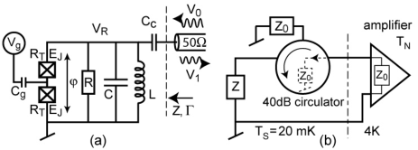
Figure 1: The L-SET resonator (a), and its equivalent circuit (impedance $Z$) coupled to cabling (b).

The coupling capacitor, typically $C_{c}\ll C$, allows, in principle, for an arbitrarily high loaded quality factor $Q_{L}$. If directly coupled to feedline, $Q_{L}=Z_{0}\sqrt{C/L_{\mathrm{tot}}}\approx 1$, which is clearly intolerable. With a coupling capacitor, however, $Q_{L}=1/2Q_{i}$ in the optimal case (as shown later) of critical coupling $Z=Z_{0}$ ($Q_{i}$ is the internal $Q$-value). The resistor $R$ is a model component for internal losses.

We consider only the linear regime, where the detector works by converting charge to resonant frequency. We do not model the ”anharmonic” operation mode lset where $\varphi$ oscillates in the nonlinear regime of the Josephson potential, yielding in fact better sensitivities in experiment.

Impedance of the L-SET circuit as illustrated in Fig. 1 is

$$Z=\frac{1}{i\omega C_{c}}+\left(i\omega C+\frac{1}{i\omega L}+\frac{1}{i\omega L_{J}}+\frac{1}{R}\right)^{-1}.$$ (1)

The circuit is probed by measuring the voltage reflection coefficient $\Gamma=|\Gamma|\exp(i\arg(\Gamma))=(Z-Z_{0})/(Z+Z_{0})$ to an incoming voltage wave of amplitude $V_{0}$. The reflected wave amplitude is $V_{1}=|\Gamma|V_{0}$. Here, $Z_{0}=50\,\Omega$ is the wave impedance of coaxial lines.

Spectral density of noise power at the output of the 1st stage amplifier, referred to amplifier input, is $k_{B}T_{N}^{*}$, where the effective temperature $T_{N}^{*}$ is due to amplifier noise and sample noise: $T_{N}^{*}=T_{N}+T_{S}$. Sample is supposed to be critically coupled, and hence its noise is like that of a $50\,\Omega$ resistor at the temperature $T_{S}$ (note that the Josephson effect is a system ground state property and hence it contributes no noise). Typically, $k_{B}T_{S}\lesssim\hbar\omega_{p}$, and thus sample noise is already in the quantum limit.

Noise of contemporary rf-amplifiers, however, remains far from the quantum limit, i.e., $T_{N}\gg T_{S}$. The best demonstrated SQUID-based rf-amplifiers have reached $T_{N}\sim 100-200$ mK squid . Therefore, added noise from the sample can be safely ignored when analyzing detector performance.

Charge sensitivity for amplitude modulation (AM) of the rf-SET was calculated in detail in Ref. leif assuming detection of one sideband. It was assumed that the sensitivity is limited by general equivalent noise temperature similarly as here, and hence the formula applies as such:

$$s_{q}=\sqrt{2k_{B}T_{N}}/\left(V_{0}\frac{\partial|\Gamma|}{\partial q}\right).$$ (2)

In the linear regime, the best sensitivity of the L-SET is clearly at the largest acceptable value of $V_{0}$, where linearity still holds reasonably well. This is the case when an AC current of critical current peak value flows through the SCPT, and the phase swing is $\pi$ p-p. Then, voltage across the SCPT, and resonator (later we discuss important quantum corrections to this expression), $V_{R}=\left|2Z_{R}/(Z+Z_{0})\right|V_{0}$ equals a universal critical voltage of a Josephson junction MSthesis , $V_{C}=\pi\hbar\omega/(4e)\simeq 3\,\mu$V at $f_{p}=1$ GHz. Here, $Z_{R}$ is impedance of the parallel resonator.

We decompose the derivative in Eq. (2) into terms due to the circuit and SCPT: $\frac{\partial|\Gamma|}{\partial q}=\frac{\partial|\Gamma|}{\partial\omega_{p}}\frac{\partial\omega_{p}}{\partial L_{J}}\frac{\partial L_{J}}{\partial q}$. We define a dimensionless transfer function $g^{\prime}=(\partial L_{J}/\partial q)(e/L_{J0})$ scaled according to minimum (w.r.t. gate) of $L_{J}$. The gate value which yields the maximum of $g^{\prime}$, denoted $g$, is the optimum gate DC operation point of the charge detector. In what follows, $L_{J}$ should be understood as its value at this point. With a given $E_{J}/E_{C}$ ratio, we compute the values of $g$ and $L_{J}$ numerically from the SCPT band structure ($g$ is plotted in Fig. 4 in Ref. lset ). If $E_{J}/E_{C}\ll 1$, one can use the analytical result $L_{J0}=2\Phi_{0}^{2}/(\pi E_{J})$.

With a general choice of parameters of the tank resonator, Eq. (2) needs to be evaluated numerically. However, when the system is critically coupled, $Z=Z_{0}$, a simple analytical formula can be derived. Numerical calculations of Eq. (2) over a large range of parameters show that the best sensitivity occurs when $Z=Z_{0}$. This is reasonable because it corresponds to the best power transfer. All the following results are for critical coupling. Later, we examine effects of detuning from the optimum. Initially, we also suppose the oscillator is classical, i.e., its energy $E\gg\hbar\omega_{p}$.

Optimal value of the coupling capacitor is calculated using $Q_{L}=1/2Q_{i}$, and we get $C_{c}=\sqrt{C/(\omega_{p}Q_{i}Z_{0})}$.

Since it was assumed $Z=Z_{0}$, it holds that $Z_{R}=Z_{0}+i/(\omega_{p}C_{c})$. Voltage amplification by the resonator then becomes $V_{R}=V_{0}\sqrt{Q_{i}/(\omega_{p}Z_{0}C)}$ which holds for a reasonably large $Q_{i}$. We thus have $V_{0}=\pi\hbar\omega_{p}^{3/2}\sqrt{Z_{0}C}/(4e\sqrt{Q_{i}})$.

With $\omega_{p}=(L_{\mathrm{tot}}C)^{-1/2}$, we get immediately $(\partial\omega_{p}/\partial L_{J})^{-1}=2\sqrt{C}L_{J}^{2}\sqrt{1/L+1/L_{J}}$. Using the fact qfactor that FWHM of the loaded resonance absorption dip at critical coupling is $\omega_{p}/(2Q_{L})$, we get $\partial|\Gamma|/\partial\omega_{p}=2Q_{L}/\omega_{p}=Q_{i}/\omega_{p}$.

Inserting these results into Eq. (2), we get expression for the AM charge sensitivity in the limit the oscillator is classical:

$$s_{q}=\frac{8eL_{J}^{2}\sqrt{\frac{1}{L}+\frac{1}{L_{J}}}\sqrt{2k_{B}T_{N}}}{g\pi\hbar L_{J0}\sqrt{\omega_{p}Q_{i}}}$$ (3)

in units of $[e/\sqrt{\rm Hz}]$. Clearly, the shunting inductor is best omitted, i.e., $L\rightarrow\infty$. The classical result, Eq. (3), improves without limit at low $E_{J}/E_{C}$.

We will now discuss quantum corrections to Eq. (3). Although spectral density of noise in the resonator is negligible in output, integrated phase fluctuations even due to quantum noise can be large. Integrated phase noise in a high-$Q$ oscillator is $\langle\Delta\varphi^{2}\rangle=2\pi^{2}\hbar L_{\mathrm{tot}}\omega_{p}/\Phi_{0}^{2}$ devoret . When $\langle\Delta\varphi\rangle$ exceeds the linear regime $\sim\pi$, which happens at high inductance (low $E_{J}/E_{C}$), plasma resonance ”switches” into nonlinear regime, and the gain due to frequency modulation vanishes. If $L\gg L_{J}$, and $f_{p}\sim 1$ GHz, we have ultimate limits of roughly $E_{J}/E_{C}\sim 0.06$, or $\sim 0.02$, for a SCPT made out of Al or Nb, respectively.

Even before this switching happens, quantum noise in the oscillator $E_{Q}=\frac{1}{2}\hbar\omega_{p}$ has an adverse effect because less energy can be supplied in the form of drive, that is, $V_{0}$ is smaller. This can be calculated in a semiclassical way as follows. Energy of the oscillator is due to drive ($E_{D}$) and noise (we stay in the linear regime): $E=(\Phi_{0}\varphi)^{2}/(8\pi^{2}L_{\mathrm{tot}})=E_{D}+E_{Q}=(\Phi_{0}\varphi_{D})^{2}/(8\pi^{2}L_{\mathrm{tot}})+\frac{1}{2}\hbar\omega_{p}$, where the phases are in RMS, $\varphi$ is the total phase swing, and $\varphi_{D}$ is that due to drive. Solving for the latter, we get $\varphi_{D}=\sqrt{\varphi^{2}-4\pi^{2}\hbar\omega_{p}L_{\mathrm{tot}}/\Phi_{0}^{2}}$. The optimal drive strength $V_{R}=V_{C}$ corresponds to $\sqrt{2}\varphi=\pi/2$, and hence the maximum probing voltage $V_{0}$ is reduced by a factor $\beta=\sqrt{1-32\hbar\omega_{p}L_{\mathrm{tot}}/\Phi_{0}^{2}}$ due to quantum noise in the oscillator.

The optimal sensitivity is finally

$$s_{q}^{QL}=\frac{64\sqrt{2}eL_{J}^{2}\sqrt{2k_{B}T_{N}}}{g\pi\sqrt{\hbar}\Phi_{0}L_{J0}\sqrt{Q_{i}}},$$ (4)

which depends only weakly on operation frequency. We optimized Eq. (2) (replacing there $V_{0}$ by $\beta V_{0}$) assuming similar tunnel junction properties as in the experiment, $E_{J}E_{C}=1.8$ K² (Al) and $E_{J}E_{C}=10$ K² (Nb). The results are plotted in Fig. 2 together with corresponding power dissipation $(V_{C}/\sqrt{2})^{2}/R=\pi^{2}\hbar^{2}\omega_{p}/(32e^{2}Q_{i}L_{J})$.

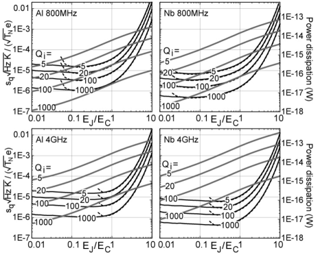
Figure 2: Charge sensitivity of the L-SET optimized from Eq. (2) (black lines). The analytical result (Eq. (3) multiplied by $\beta^{-1}$), with $L=\infty$, is shown with dashed lines. Gray lines are the corresponding power dissipation. All the graphs have the same scales, which are indicated for $s_{q}$ (left) and dissipation (right). The curves are for different $Q_{i}$ as marked. All graphs have $Z\simeq Z_{0}$.

The optimal sensitivity is reached around $E_{J}/E_{C}\simeq 0.1...0.3$, where the curves in Fig. 2 almost coincide Eq. (4). $C_{c}$ should be chosen so that critical coupling results. Typically also it should hold $L\gg L_{J}$ (see the analytical curve in Fig. 2). However, sensitivity decreases only weakly if these values are detuned from their optimum (Fig. 3).

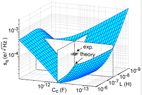
Figure 3: Measured charge sensitivity (box) compared to calculations. In experiment, $C_{c}\sim 0.5$fF, and $L\sim 28$nH. The graph shows also how the sensitivity would change as a function $C_{c}$ and $L$ according to the model.

By numerical investigation we found that readout of $\arg(\Gamma)$, with mixer detection, offers within accuracy of numerics the same numbers than the discussed AM (readout of $|\Gamma|$).

In experiment, we measured charge sensitivity for the following sample and resonator: $R_{T}\simeq 11$ k$\Omega$, $E_{J}\simeq 0.7$ K, $E_{C}\simeq 2.6$ K, $E_{J}/E_{C}\simeq 0.3$, $Q_{i}\simeq 16$, $L\simeq 28$ nH, $C\simeq 1.2$ pF, $C_{c}\simeq 0.5$ pF. In all samples so far, $Q_{i}\lesssim 20$ which is presently not understood. The measurements were done as described in Ref. lset , with $T_{N}\sim 5$ K amplifier . We measured $s_{q}=7\times 10^{-5}$e$/\sqrt{\mathrm{Hz}}$ by AM at 1 MHz, while a prediction with the present parameters is $s_{q}=3\times 10^{-5}$e$/\sqrt{\mathrm{Hz}}$ (see also Fig. 3).

Theory and experiment thus agree reasonably. The somewhat lower sensitivity in experiment is likely to be due to external noise which forces a lower $V_{0}$ and also smoothes out the steepest modulation. Its origin is not clear. Also the $25\%$ higher values of $L_{J}$ than expected agree qualitatively with noise.

In the ”anharmonic” mode, we measured $s_{q}=3\times 10^{-5}$e$/\sqrt{\mathrm{Hz}}$, with a usable bandwidth of about 100 MHz ($s_{q}\sim 10^{-4}$e$/\sqrt{\mathrm{Hz}}$ at 100 MHz). Considering both $s_{q}$ and band, a performance comparable to the best rf-SETs rfset ; chalmers has been reached with the L-SET, though here at more than two orders of magnitude lower power dissipation ($\sim 10$ fW).

In the linear regime, the power lost $P_{\Sigma}$ from drive frequency $m=1$ to higher harmonics is determined by the sum, for $m\geq 2$, of Josephson junction admittance components $|Y_{m}|=2J_{m}\left(2e/(\hbar\omega)V_{1}\right)$. At the critical voltage $V_{1}=V_{C}$, this amounts to $Y_{\Sigma}/Y_{1}=P_{\Sigma}/P_{1}\sim 30$ %. Since charge sensitivity is proportional to square root of power, it thus decreases only $\sim 15$ % due to non-linearity. Further corrections due to slightly non-sinusoidal lowest band of the SCPT, as well as asymmetry due to manufacturing spread in junction resistance, we estimate as insignificant.

Next we discuss non-adiabaticity. Interband Zener transitions might make the SCPT jump off from the supposed ground band 0. We make a worst case estimate by assuming that the drive is $2\pi$ p-p (partially due to noise). The probability to cross the minimum $\Delta_{m}$ of band gap $\Delta=E_{1}-E_{0}$ is: $P_{Z}\simeq\exp\left(-\pi\Delta_{m}^{2}/(2\hbar D\dot{\varphi})\right)$, where we evaluate the dependence of the band gap on phase $D=\partial\Delta/\partial\varphi$ at $\varphi=\pi/2$. $\dot{\varphi}=2\omega_{p}$ is determined by the drive.

Zener tunneling is significant if it occurs sufficiently often in comparison to $1\rightarrow 0$ relaxation. Threshold is when $P_{Z}\sim\Gamma_{\downarrow}/(2f_{0})$, where $\Gamma_{\downarrow}\gtrsim(1\mu\rm{s})^{-1}$ is the relaxation rate. Operation of the L-SET can thus be affected above $P_{Z}\sim 10^{-4}$.

Numerical calculations for $P_{Z}$ show that Zener tunneling is exponentially suppressed, at the L-SET optimal working point, in the interesting case of low $E_{J}/E_{C}$ MSthesis . This is because $\Delta_{m}$ becomes large and $D$ small. For instance, if $E_{J}=1$ K and $f_{p}=1$ GHz, we got that Zener tunneling is insignificant below $E_{J}/E_{C}\sim 3$. With $E_{J}=0.5$ K and $f_{p}=5$ GHz, the threshold is $E_{J}/E_{C}\simeq 1$.

We conclude that with sufficiently high $Q_{i}$ and using a amplifier close to the quantum limit, even $s_{q}\sim 10^{-7}$e$/\sqrt{\mathrm{Hz}}$, order of magnitude better than the shot-noise limit of rf-SET, is intrinsically possible for the L-SET. So far, the sensitivity has been limited by $Q_{i}\lesssim 20$.

Fruitful discussions with M. Feigel’man, U. Gavish, T. Heikkilä, R. Lindell, H. Seppä are gratefully acknowledged. This work was supported by the Academy of Finland and by the Large Scale Installation Program ULTI-3 of the European Union (contract HPRI-1999-CT-00050).

References

- (1) Y. Nakamura, Yu. A. Pashkin, and J. S. Tsai, Nature 398, 786 (1999).
- (2) D. Vion et al., Science 296, 886 (2002).
- (3) Y. Yu, S. Han, X. Chu, S. Chu, and Z. Wang, Science 296, 889 (2002).
- (4) A. Wallraff et al., Nature 431, 162 (2004).
- (5) M. A. Sillanpää, L. Roschier, and P. J. Hakonen, Phys. Rev. Lett. 93, 066805 (2004).
- (6) R. J. Schoelkopf et al., Science 280, 1238 (1998).
- (7) M. A. Sillanpää, L. Roschier, and P. J. Hakonen, submitted to Proceedings of the Vth Rencontres de Moriond in Mesoscopic Physics (2004).
- (8) A. N. Korotkov and M. A. Paalanen, Appl. Phys. Lett. 74, 4052 (1999).
- (9) A. B. Zorin, Phys. Rev. Lett. 86, 3388 (2001).
- (10) M.-O. André et al., Appl. Phys. Lett. 75, 698 (1999).
- (11) L. Roschier et al., J. Appl. Phys. 95, 1274 (2004).
- (12) M. A. Sillanpää, Ph. D. thesis, Helsinki University of Technology (2005).
- (13) D. Kajfez, Q Factor (Vector Fields, Oxford, 1994).
- (14) M. Devoret, in Les Houches, Session LXIII, eds. S. Reynaud, E. Giacobino and J. Zinn-Justin (Elsevier, Amsterdam, 1997).
- (15) L. Roschier and P. Hakonen, Cryogenics 44, 783 (2004).
- (16) A. Aassime, D. Gunnarsson, K. Bladh, P. Delsing, and R. Schoelkopf Appl. Phys. Lett. 79, 4031 (2001).