Current-induced nonequilibrium vibrations in single-molecule devices

Abstract

Finite-bias electron transport through single molecules generally induces nonequilibrium molecular vibrations (phonons). By a mapping to a Fokker-Planck equation, we obtain analytical scaling forms for the nonequilibrium phonon distribution in the limit of weak electron-phonon coupling $\lambda$ within a minimal model. Remarkably, the width of the phonon distribution diverges as $\sim\lambda^{-\alpha}$ when the coupling decreases, with voltage-dependent, non-integer exponents $\alpha$. This implies a breakdown of perturbation theory in the electron-phonon coupling for fully developed nonequilibrium. We also discuss possible experimental implications of this result such as current-induced dissociation of molecules.

I Introduction

The vision of molecular electronicsAviram and Ratner (1974) in part depends on the realization of devices such as molecular transistors, switches, or diodes. One strategy towards this goal involves the coupling of electronic and vibrational (phononic) degrees of freedom of molecules. Experiments with single-molecule devices have demonstrated effects of electron-phonon coupling in current-voltage characteristics ($IV$s),Park et al. (2000); Smit et al. (2002); Yu et al. (2004) and a number of theoretical studies have investigated such features in $IV$s,McCarthy et al. (2003); Mitra et al. (2004); Braig and Flensberg (2004); Galperin et al. (2004); Chen et al. (2004); Koch and von Oppen (2004) shot noise,Mitra et al. (2004); Koch and von Oppen (2004) and the thermopowerKoch et al. (2004) as well as applications such as diodesKaat and Flensberg (2004) and switches.Cizek et al. (2004)

A question of principal importance for single-molecule devices are the consequences of nonequilibrium effects at finite bias. Strong nonequilibrium molecular vibrations can be beneficial in molecular devices, e.g., by enhancing switching rates between molecular conformations. In other instances, they may hinder the operation of devices, in the extreme case by inducing dissociation of the molecule. Recent theoretical work shows that even within simple models, vibrational nonequilibrium has important effects on $IV$s and shot noise,Aji et al. (2003); Mitra et al. (2004) may induce a shuttling instability,Fedorets et al. (2004); Novotný et al. (2004) or lead to current flow characterized by a self-similar hierarchy of avalanches of large numbers of transferred electrons.Koch and von Oppen (2004)

Recent numerical results by Mitra et al.Mitra et al. (2004) suggest that intriguingly, vibrational nonequilibrium becomes stronger as the electron-phonon coupling $\lambda$ decreases. Characterizing the vibrational nonequilibrium by the probability distribution of phonon excitations, these authors observe that the width of this distribution grows with decreasing coupling $\lambda$. These numerical results are obtained within a minimal model describing transport through one molecular orbital, which is coupled to a single vibrational mode.

In this paper, we first clarify the underlying mechanism for this nonequilibrium effect by developing an analytical theory. Our approach relies on a mapping to a Fokker-Planck equation, which becomes exact in the limit of weak electron-phonon coupling. This mapping predicts that the width at half maximum (WHM) of the phonon distribution diverges as $\lambda\to 0$. Remarkably, the WHM is shown to scale as $\lambda^{-\alpha}$ with bias-dependent, non-integer exponents $\alpha>0$. We confirm our analytical results by numerical simulations.

“Real” single-molecule devices will typically involve features such as several vibrational modes, anharmonic vibrational potentials, and direct vibrational relaxation (e.g. due to radiation or interaction with the substrate), which are not fully captured by the minimal model. We therefore discuss how various such extensions of the minimal model, which may be important for an accurate description of experimental systems, modify our analytical findings. Specifically, we include anharmonic vibrations within a Morse-potential model which allows us to discuss current-induced dissociation of the molecule. In this context, we show that the current-induced dissociation rate is governed by an interplay of the above-mentioned divergence of the width of the phonon distribution and a slowing down of the diffusion in phonon space as $\lambda$ decreases.

The outline of the paper is as follows: In Sec. II we discuss the nonequilibrium effects of weak electron-phonon coupling within the minimal model. The model is specified in II.1, and the resulting properties of the phonon distribution are derived in II.2. Nonequilibrium properties of “real” molecules are discussed in Sec. III by going beyond the minimal model. In particular, we address the effects of vibrational relaxation and the presence of several phonon modes as well as the situation of anharmonic potentials in III.1, III.2 and III.3, respectively. Our conclusions are summarized in Sec. IV.

II Weak electron-phonon coupling within the minimal model

II.1 Reduced model

We investigate the nonequilibrium vibrational properties of a molecule coupled to metallic source and drain electrodes under finite bias within the following minimal model.Glazman and Shekhter (1988); Boese and Schoeller (2001); Mitra et al. (2004); Koch et al. (2004) Electronic transport is taken to result from sequential tunneling through one spin-degenerate molecular orbital with energy $\varepsilon$, which is measured relative to the zero-bias Fermi energies of the leads and which can be tuned by a gate voltage. As a minimal model, we consider a single vibrational mode with frequency $\omega$. [Typical vibrational energies in molecules are of the order of 0.1 eV.] The system’s Hamiltonian reads $H=H_{\text{mol}}+H_{\text{leads}}+H_{\text{mix}}$, where

$$H_{\text{mol}}= \varepsilon n_{d}+\frac{U}{2}n_{d}(n_{d}-1)$$ (1)

$$+\lambda\hbar\omega(b^{\dagger}+b)n_{d}+\hbar\omega(b^{\dagger}b+1/2)$$

describes the molecular degrees of freedom, $H_{\text{leads}}$ a free electron gas in the leads $a=L,R$ (with creation operators $c^{\dagger}_{a\mathbf{p}\sigma}$), and

$$H_{\text{mix}}=\sum_{a=L,R}\sum_{\mathbf{p},\,\sigma}\left(t_{a}c^{\dagger}_{a\mathbf{p}\sigma}d_{\sigma}+\text{h.c.}\right)$$ (2)

the tunneling between leads and molecule.

We focus on the regime of strong Coulomb blockade, appropriate when voltage and temperature are small compared to the charging energy $U$. The operator $d_{\sigma}$ ($d_{\sigma}^{\dagger}$) annihilates (creates) an electron with spin projection $\sigma$ on the molecule, $n_{d}=\sum_{\sigma}d_{\sigma}^{\dagger}d_{\sigma}$ denotes the corresponding occupation-number operator. Vibrational excitations are annihilated (created) by $b$ ($b^{\dagger}$). The electron-phonon coupling term can be eliminated by a canonical transformation,Mitra et al. (2004); Glazman and Shekhter (1988) leading to a renormalization of the parameters $\varepsilon$ and $U$, and of the lead-molecule coupling $t_{a}\rightarrow t_{a}\exp[-\lambda(b^{\dagger}-b)]$. From now on, we refer to the renormalized parameters as $\varepsilon$ and $U$.

The coupling between molecule and leads is parameterized by the tunneling matrix elements $t_{L}$ and $t_{R}$, and it is assumed to be weak in the sense that the energy broadening $\Gamma$ of molecular levels is small, i.e. $\Gamma\ll k_{B}T,\hbar\omega$, so that a perturbative treatment for $H_{\text{mix}}$ in the framework of rate equations, as introduced in the context of Coulomb blockade phenomena,Beenakker (1991) is appropriate. We focus on temperatures $k_{B}T\ll\hbar\omega$ (corresponding to typical low-temperature experiments, see e.g. Ref. Smit et al., 2002). For simplicity, we assume a symmetric device with $t_{L}=t_{R}\equiv t_{0}$ and identical voltage drops of $V/2$ across each junction.

Then, the occupation probability $P^{n}_{q}$ for the molecular state $\left|\,n,q\,\right\rangle$ with $n$ electrons and $q$ phonons is determined by the rate equations

$$\frac{dP^{n}_{q}}{dt}=\sum_{n^{\prime},q^{\prime}}\left[P^{n^{\prime}}_{q^{\prime}}W^{n^{\prime}\rightarrow n}_{q^{\prime}\rightarrow q}-P^{n}_{q}W^{n\rightarrow n^{\prime}}_{q\rightarrow q^{\prime}}\right].$$ (3)

(The discussion of direct phonon relaxation is deferred until later in this paper.) The transition rates $W^{n\rightarrow n^{\prime}}_{q\rightarrow q^{\prime}}$ obtained by Fermi’s golden rule are proportional to the square of the Franck-Condon (FC) matrix element

$$M_{q\rightarrow q^{\prime}}=\int_{-\infty}^{\infty}dx\,\phi_{q^{\prime}}(x)\phi_{q}(x-\sqrt{2}\lambda\ell_{\text{osc}}),$$ (4)

i.e. the overlap of two harmonic oscillator wavefunctions $\phi_{q}(x)$, shifted relative to each other by a distance $\sqrt{2}\lambda\ell_{\text{osc}}$, with electron-phonon coupling strength $\lambda$, and vibrational oscillator length $\ell_{\text{osc}}=(\hbar/M\omega)^{1/2}$. Based on spectral data for diatomic molecules,Huber and Herzberg (1979) one can find electron-phonon coupling strengths ranging between $\lambda\simeq 0.01$ (BeO) and $\lambda\simeq 5.4$ (Kr₂). The FC matrix elements can be expressed as

$$M_{q\rightarrow q^{\prime}}=\left(q!/Q!\right)^{1/2}\\ \lambda^{Q-q}e^{-\lambda^{2}/2}\,L_{q}^{Q-q}\left(\lambda^{2}\right)\operatorname{sgn}(q-Q)^{q-Q},$$ (5)

see e.g. Ref. Koch et al., 2004, where $L^{n}_{m}(x)$ denotes the generalized Laguerre polynomial.

II.2 Phonon distributions for weak electron-phonon coupling

For $\lambda\ll 1$, Eq. (5) leads to

$$\left|M_{q_{1}\rightarrow q_{2}}\right|^{2}\simeq\frac{Q!}{q!}\frac{\lambda^{2\Delta q}}{(\Delta q!)^{2}},$$ (6)

valid for $q\lambda^{2},\,\Delta q\lambda^{2}\ll 1$, where $Q=\max\{q_{1},q_{2}\}$, $q=\min\{q_{1},q_{2}\}$, and $\Delta q=Q-q$. Therefore, the FC matrix elements and the transition rates $W^{n\rightarrow n\pm 1}_{q\rightarrow q^{\prime}}$ decay rapidly with increasing $\Delta q$. Consequently, the vibrational state of the molecule is predominantly changed by processes for which $q\rightarrow q^{\prime}=q\pm 1$, and $\Delta q=1$. Neglecting all other processes, Eq. (3) describes a random walk in the space of phonon states $q$ with $q$-dependent nearest-neighbor hopping rates. In this approximation, the random walker would eventually escape to infinity, as the rates for $q\rightleftharpoons q+1$ are equal and grow with $q$. This implies that there is no steady-state phonon distribution $P_{q}=\sum_{n}P^{n}_{q}$ within this random-walk model.

To derive the actual steady-state phonon distribution, it is therefore imperative to go beyond the random-walk model by including higher-order processes with $\Delta q>1$. These may favor vibrational de-excitation processes since the applied voltage sets an upper limit to the increase (but not to the decrease!) in the vibrational excitation $q$ by a tunneling event. For example, for $\epsilon=0$ the full voltage drop $eV/2$ per sequential-tunneling event can be converted into vibrational energy. Thus, $\Delta q_{a}=\lfloor eV/2\hbar\omega\rfloor+1$ is the leading-order asymmetric process for which only de-excitation processes are permitted. (Here, $\lfloor r\rfloor$ denotes the largest integer smaller or equal to $r$.)

We can now derive the scaling of the steady-state phonon distribution $P_{q}$ with electron-phonon coupling $\lambda$ by balancing the diffusion process due to tunneling events with $\Delta q=1$ [with diffusion constant $\sim q\lambda^{2}$, see Eq. (6)] and the leading asymmetric drift process [with rate $(q\lambda^{2})^{\Delta q_{a}}$, see Eq. (6)]. This leads to the balance equation

$$q\lambda^{2}{P_{q}}^{\prime\prime}\sim(q\lambda^{2})^{\Delta q_{a}}{P_{q}}^{\prime}$$ (7)

which implies a scaling law for the width $q_{0}$ of $P_{q}$, namely

$$q_{0}\sim\lambda^{-\alpha},\qquad\alpha={2(\Delta q_{a}-1)}/{\Delta q_{a}}.$$ (8)

This power-law scaling is nicely confirmed by numerical results for $P_{q}$ as shown in Fig. 1(a). Remarkably, for $k_{B}T\ll\hbar\omega$ the discrete dependence of the leading asymmetric process on bias and gate voltage implies finite regions in the $(V,\epsilon)$-plane characterized by certain non-integer exponents $\alpha$. This “phase diagram” is shown in Fig. 1(b) where the wedge-shaped regions A, B, and C correspond to $\alpha=1,4/3$, and $3/2$, respectively.

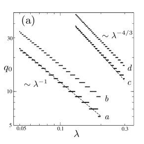
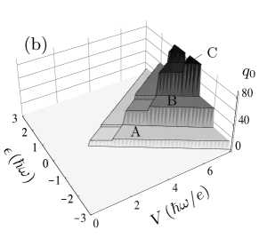
Figure 1: (a) Scaling behavior of the phonon distribution width as a function of electron-phonon coupling for representative values of $(eV/\hbar\omega,\epsilon/\hbar\omega)$ equal to a: $(3,0)$; b: $(5,1)$; c: $(5,0)$; d: $(7,1)$. (b) Width of the phonon distribution as a function of bias and gate voltage at $\lambda=0.15$ and $k_{B}T=0.005\hbar\omega$. The scaling of the width differs for the plateaus according to A: $q_{0}\sim\lambda^{-1}$, B: $q_{0}\sim\lambda^{-4/3}$, and C: $q_{0}\sim\lambda^{-3/2}$.

For the diamond-shaped regions along the line $\epsilon=0$ in Fig. 1(b), we can go beyond the derivation of this scaling behavior and obtain analytical results for the entire phonon distribution $P_{q}$ by a mapping to a Fokker-Planck equation. The derivation exploits the crucial observation that for $U\to\infty$ and $k_{B}T\ll\hbar\omega$, the transition rates $W^{n\rightarrow n^{\prime}}_{q\rightarrow q^{\prime}}=s^{n\rightarrow n^{\prime}}w_{q\rightarrow q^{\prime}}$ factorize into a spin factor $s^{n\rightarrow n^{\prime}}=(1+\delta_{n^{\prime},1})\delta_{\left|n-n^{\prime}\right|,1}$ and a phonon factor

$$w_{q\rightarrow q^{\prime}}=\tau_{0}^{-1}\left|M_{q\rightarrow q^{\prime}}\right|^{2}[\theta(q+\Delta q_{a}-1-q^{\prime})+\theta(q-q^{\prime}-\Delta q_{a})],$$ (9)

where $\tau_{0}^{-1}=\Gamma/\hbar=2\pi\rho\left|t_{0}\right|^{2}/\hbar$. In the stationary case, this implies the factorization $P^{n}_{q}=P^{n}P_{q}$, which allows us to derive the purely phononic rate equation

$$0=dP_{q}/dt=\sum_{q^{\prime}}[P_{q^{\prime}}w_{q^{\prime}\rightarrow q}-P_{q}w_{q\rightarrow q^{\prime}}],$$ (10)

Since the phonon distribution becomes wide, we can take $q$ to be continuous, expand $P_{q^{\prime}}$ around $q^{\prime}=q$ up to second order, and keep only the leading-order contributions to diffusion and drift. In this way we obtain the Fokker-Planck equation

$$0=\frac{\partial P}{\partial t}=\frac{1}{2}\frac{\partial^{2}}{\partial q^{2}}\left[D(q)P(q)\right]-\frac{\partial}{\partial q}\left[A(q)P(q)\right],$$ (11)

with diffusion coefficient $D(q)=2q\lambda^{2}/\tau_{0}$, drift coefficient $A(q)=[\lambda^{2}-c(q\lambda^{2})^{\Delta q_{a}}]/\tau_{0}$, and $c=2\Delta q_{a}(\Delta q_{a}!)^{-2}$. Remarkably, the stationary Fokker-Planck equation (11) can be solved analytically for any $\Delta q_{a}$ by the scaling ansatz $P_{q}=a\lambda^{\alpha}f(\lambda^{\alpha}q)$ with a normalization constant $a$. The universal function $f$ is uniquely determined by Eq. (11) together with the boundary conditions $f(0)=1$, $f^{\prime}(0)=0$, and we find

$$f(x)=\exp\left[-x^{\Delta q_{a}}/b\right]$$ (12)

with $b=\frac{1}{2}(\Delta q_{a}!)^{2}$. Note that in particular, this analytical result confirms the power-law scaling (8) of the width of the phonon distribution. The power-law scaling (8) together with the analytical phonon distributions (12) constitute the central results of this paper. The phonon distributions are nicely confirmed by numerical solutions of the full rate equations as shown in Fig. 2.

In fully developed nonequilibrium, the width of the phonon distribution diverges with decreasing electron-phonon coupling $\lambda$, and the resulting phonon distributions are non-analytic in $\lambda$. An important theoretical implication of this result is that in fully developed nonequilibrium, perturbation theory in the electron-phonon coupling parameter $\lambda$ is inadequate. Indeed, we find below that the radius of convergence of such an expansion in $\lambda$ would involve the direct vibrational relaxation rate.

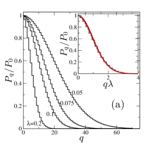
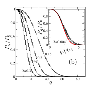
Figure 2: (Color online) Phonon distributions $P_{q}$ at bias voltages (a) $eV=3\hbar\omega$ and (b) $eV=5\hbar\omega$, plotted for several coupling strengths $\lambda$ at $\epsilon=0$, $k_{B}T=0.05\hbar\omega$. The insets show that these distributions (approximately) collapse to universal curves given by the red (dark gray) smooth curves, which are the solutions of the the Fokker-Planck equation (11) specific to each voltage range $n\hbar\omega<eV/2<(n+1)\hbar\omega$.

III Implications for “real” molecules

Transport through “real” molecules will typically involve physics that goes beyond the minimal model. In particular, we will discuss (i) direct vibrational relaxation, (ii) the presence of more than one vibrational mode, and (iii) anharmonic vibrational potentials. We show that while the exact scaling results for phonon distributions are specific to the minimal model, nonequilibrium effects at weak electron-phonon coupling persist and can be understood within the phonon diffusion model as long as the vibrational relaxation rate remains small compared to $I/e$.

III.1 Direct vibrational relaxation

Direct phonon relaxation can be included within the relaxation-time approximation by adding $-\frac{1}{\tau}[{\textstyle P^{n}_{q}-P^{\text{eq}}_{q}\sum_{q^{\prime}}P^{n}_{q^{\prime}}}]$ to the r.h.s. of the rate equations (3). Here, $P^{\text{eq}}_{q}$ denotes the equilibrium phonon distribution, which can be approximated by $P^{\text{eq}}_{q}=\delta_{q,0}$ for $k_{B}T\ll\hbar\omega$.

To understand the effect of direct vibrational relaxation on the phonon distribution $P_{q}$, it is important to note that the diffusion and drift processes in phonon space slow down as the electron-phonon coupling $\lambda$ decreases. As $\lambda$ decreases, we therefore expect that there exists a crossover coupling $\lambda_{0}$: For $\lambda\gg\lambda_{0}$, the vibrational diffusion is limited by the drift in phonon space induced by the asymmetry between vibrational excitation and de-excitation, as discussed above. By contrast, for $\lambda\ll\lambda_{0}$, the dominant limiting process is direct vibrational relaxation, leading to a decrease of the width of the phonon distribution. This expectation is confirmed by numerical results as seen in Fig. 3(a) which shows the width of the phonon distribution as a function of $\lambda$ for various relaxation rates. Fig. 3(b) shows the dependence of $\lambda_{0}$ on relaxation time $\tau$ for $\Delta q_{a}=1$. Note that $\lambda_{0}$ grows only very slowly with increasing relaxation. While the $\lambda_{0}$ vs. $\tau$ dependence is close to a power law with an exponent $1/4$ - $1/3$, no simple scaling can be expected. The reason is that the scaling suggested by the rate equation (3) amended by the relaxation term is incompatible with the scaling implied by the boundary condition $\lambda^{2(\alpha+1)}f^{\prime}(0)=-\tau_{0}/\tau Sa$ at $q=0$, where $S=1+P^{0}$.

III.2 Additional vibrational modes

Typical molecules have many vibrational modes of different vibrational frequencies. We expect that the scenario of the minimal model is most relevant to molecules whose lowest frequency mode happens to be weakly coupled. As this mode becomes highly excited, it would start to mix with other (higher-frequency) modes. In the simplest approximation, we can account for such mode mixing as a channel of direct vibrational relaxation so that the discussion of the previous subsection applies. Indeed, due to this mixing, vibrational energy can be distributed among different modes, which will generally tend to decrease phonon occupation numbers, similar to the vibrational relaxation discussed above. Under these conditions, such a weakly coupled vibrational mode may provide an efficient pathway to “pump” higher-frequency vibrations.

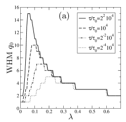
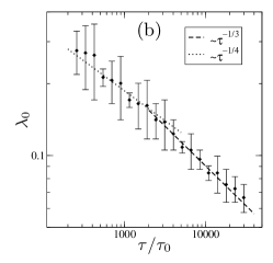
Figure 3: (a) Width of the phonon distribution as a function of electron-phonon coupling strength for several vibrational relaxation times $\tau$ and $eV=3\hbar\omega$, $k_{B}T=0.05\hbar\omega$, $\epsilon=0$. For $\lambda>0.25$ all curves show the approximate $q_{0}\sim\lambda^{-1}$ scaling. Below a relaxation-rate dependent crossover-point $\lambda_{0}$ the WHM is strongly suppressed due to direct relaxation. (b) Crossover-point $\lambda_{0}$ vs. relaxation time $\tau$.

III.3 Morse potential and dissociation

So far, our considerations were based on the harmonic approximation for the phonon potential. We argue however that wide phonon distributions are not an artefact of this approximation, but also appear for more realistic, anharmonic potentials. As an example, we investigate the effect of weak electron-phonon coupling for the Morse potential

$$V(x)=D\left[e^{-2\beta(x-x_{0})}-2e^{-\beta(x-x_{0})}\right],$$ (13)

where $D>0$ denotes the dissociation energy, $\beta$ the inverse range, and $x_{0}$ the potential minimum.

The Morse potentialMorse (1929) accurately describes the vibrations of diatomic molecules and allows us to study current-induced molecular dissociation.Seideman (2003) This phenomenon has been explored experimentally in STM experiments with molecules on metal surfaces, and sufficiently high currents have been reported to lead to fast dissociation of the absorbed molecules.Stipe et al. (1997) While this scenario with strong coupling between the molecule and the metal surface is distinct from the regime addressed in this paper, we remark that, in principle, the deposition of molecules on passivated surfacesQiu et al. (1997) can be exploited to study the weak-coupling regime as well.

In analogy to the harmonic oscillator model, we assume that the potential energy curves for the neutral and singly-charged molecule have the same shape (i.e. $D$ and $\beta$ are fixed), but are shifted with respect to each other by $\Delta x=\sqrt{2}\lambda\ell_{\text{osc}}$. Building on e.g. Ref. Lemus et al., 2004, we derive Franck-Condon matrix elements for the Morse potential, analogous to Eq. (4), between bound states as well as between bound and continuum states. Details of this calculation are referred to Appendix .

Specifically, we study the current-induced dissociation rate of the molecule as function of electron-phonon coupling and bias voltage by Monte-Carlo simulation. Assuming low temperatures and switching on the voltage at $t=0$, the molecule starts in the phonon ground state and then evolves in time due to the tunneling dynamics. Given that transitions from the continuum back to bound states are negligible, we obtain an average dissociation rate $\Gamma_{\text{diss}}$ by recording the times $t_{\text{diss},i}$ required for reaching the continuum and averaging over samples. (We note that calculations of mean first-passage times for the highest-lying bound level give compatible dissociation times.) Typical results for dissociation rates for weak electron-phonon couplings (without relaxation) are depicted in Fig. 4.

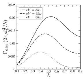
Figure 4: Mean dissociation rate as a function of electron-phonon coupling strength at $k_{B}T=0.005\hbar\omega$ for several bias voltages as obtained by Monte Carlo simulation with a Morse potential containing 10 bound states.

The maximum in the dissociation rate $\Gamma_{\rm diss}$ vs. $\lambda$ can be understood as a direct consequence of a competition between the broadening of the phonon distribution and the slowing down of diffusion in phonon space. As $\lambda$ decreases from values of the order of unity, $\Gamma_{\rm diss}$ first increases. This reflects the concurrent increase in the width of the phonon distribution. Beyond the maximum, $\Gamma_{\rm diss}$ decreases due to the slowing down of diffusion in phonon space. Finally, the dissociation rate increases with voltage because of the increased width of the phonon distribution (see Fig. 1) and the possibility of multiple-phonon excitations within one tunneling event.

IV Conclusions

We have studied the current-induced vibrational nonequilibrium in single-molecule devices and found that remarkably, the width of the nonequilibrium phonon distribution increases with decreasing electron-phonon coupling. We have identified regions in the bias voltage-gate voltage plane in which the width of the phonon distribution exhibits power-law divergences with decreasing $\lambda$, with voltage-dependent non-integer exponents. In some representative cases, we are able to derive analytical phonon distributions by a mapping to a Fokker-Planck equation. These striking effects of current-induced nonequilibrium are found to have important implications in more realistic models which include direct vibrational relaxation and anharmonic potential surfaces. A very important conclusion from our work is that approaches which are perturbative in the electron-phonon coupling $\lambda$ have to be assessed with extreme care in fully-developed nonequilibrium. Finally, we remark that recent experimentsLeRoy et al. (2004) show that the vibrational relaxation time can be as large as 10ns, in which case current-induced vibrational nonequilibrium becomes important for currents as small as 10pA.

Appendix A FC matrix elements for the Morse potential

The calculation of dissociation rates within the Morse-potential model requires not only the determination of FC matrix elements between bound states [which is straightforward and can be found, e.g., in Ref. Koch and von Oppen, 2005], but also matrix elements between bound and continuum states. Although analytical expressions for the continuum eigenfunctions of the Morse potential are known,Matsumoto (1988) their structure involves confluent hypergeometric functions with complex parameters, rendering a direct numerical evaluation of the FC matrix elements difficult.

Instead, we make use of the complete set of orthonormal functions introduced in Ref. Lemus et al., 2004,

$$\phi_{n}(x)=\sqrt{\frac{\beta n!}{\Gamma(2\sigma+n)}}L_{n}^{2\sigma-1}(y)y^{\sigma}e^{-y/2}.$$ (14)

Here, we denote $y=(2j+1)e^{-\beta x}$ and $\sigma=j-\lfloor j\rfloor$. $j$ is fixed by the Morse potential parameters to

$$2j+1=\sqrt{8\mu D/\beta^{2}\hbar^{2}},$$ (15)

and $\lfloor j\rfloor$ [which is the integer closest to and smaller than $j$] gives the number of bound states. This set of functions has three appealing properties:Lemus et al. (2004) (i) It forms a discrete complete orthonormal basis enumerated by $n=0,1,2,\ldots$. (ii) The first $\lfloor j\rfloor+1$ functions form a basis for the bound eigenstates of the Morse potential, all remaining functions span the space of continuum eigenstates. (iii) With respect to this basis, the Hamiltonian takes a particularly simple tridiagonal form.

Denoting the bound and continuum eigenstates of the Morse potential by $\left|\,\psi_{q}\,\right\rangle$ and $\left|\,\psi_{E}\,\right\rangle$, respectively, we can now calculate the relevant FC matrix element for a transition from a bound state $\left|\,\psi_{q}\,\right\rangle$ into a continuum state $\left|\,\psi_{E}\,\right\rangle$ by

$$M_{q\rightarrow E} =\left\langle\,\psi_{E}\,\left|\,e^{\sqrt{2}\lambda\ell_{\text{osc}}\frac{d}{dx}}\,\right|\,\psi_{q}\,\right\rangle$$ (16)

$$=\sum_{m=0}^{\lfloor j\rfloor}\sum_{n=\lfloor j\rfloor+1}^{\infty}\alpha_{En}^{*}\beta_{km}\left\langle\,\phi_{n}\,\left|\,e^{\sqrt{2}\lambda\ell_{\text{osc}}\frac{d}{dx}}\,\right|\,\phi_{m}\,\right\rangle.$$

Here, the expansion coefficients $\alpha_{En}$ and $\beta_{km}$ for continuum and bound eigenstates with respect to the $\{\left|\,\phi_{n}\,\right\rangle\}$ basis are obtained through numerical diagonalization of the Hamiltonian. Finally, the FC matrix for the $\{\left|\,\phi_{n}\,\right\rangle\}$ basis are given by

$$\left\langle\,\phi_{n}\,\left|\,e^{\sqrt{2}\lambda\ell_{\text{osc}}\frac{d}{dx}}\,\right|\,\phi_{n^{\prime}}\,\right\rangle=\frac{(-1)^{n^{\prime}}(4a)^{\sigma}\Gamma(n+n^{\prime}+2\sigma)}{\sqrt{\Gamma(2\sigma+n)\Gamma(2\sigma+n^{\prime})n!n^{\prime}!}}$$ (17)

$$\times\frac{(a-1)^{n+n^{\prime}}}{(a+1)^{n+n^{\prime}+2\sigma}}{{}_{2}\text{F}}_{1}\left(-n^{\prime},-n;-n-n^{\prime}-2\sigma+1;{\textstyle\frac{(1+a)^{2}}{(1-a)^{2}}}\right),$$

where $a=\exp\left[-\frac{2\lambda}{\sqrt{\lambda+1}}\right]$ and ${}_{2}F_{1}$ denotes the (Gaussian) hypergeometric function. In practice, one introduces a cutoff for the basis $\{\left|\,\phi_{n}\,\right\rangle\}$, leading to a discretization of continuum eigenstates. In order to ensure a sufficiently dense spacing of the spectrum close to the dissociation limit, we take into account $\sim 10,000$ basis functions.

References

- Aviram and Ratner (1974) A. Aviram and M. Ratner, Chem. Phys. Lett. 29, 277 (1974).
- Park et al. (2000) H. Park et al., Nature 407, 57 (2000).
- Smit et al. (2002) R. H. M. Smit et al., Nature 419, 906 (2002).
- Yu et al. (2004) L. Yu et al., Phys. Rev. Lett. 93, 266802 (2004).
- McCarthy et al. (2003) K. D. McCarthy, N. Prokof’ev, and M. T. Tuominen, Phys. Rev. B 67, 245415 (2003).
- Mitra et al. (2004) A. Mitra, I. Aleiner, and A. J. Millis, Phys. Rev. B 69, 245302 (2004).
- Braig and Flensberg (2004) S. Braig and K. Flensberg, Phys. Rev. B 70, 085317 (2004).
- Galperin et al. (2004) M. Galperin, M. A. Ratner, and A. Nitzan, Nano Lett. 4, 1605 (2004).
- Chen et al. (2004) Y.-C. Chen, M. Zwolak, and M. DiVentra, Nano Lett. 4, 1709 (2004).
- Koch and von Oppen (2004) J. Koch and F. von Oppen, Phys. Rev. Lett. 94, 206804 (2005).
- Koch et al. (2004) J. Koch, F. von Oppen, Y. Oreg, and E. Sela, Phys. Rev. B 70, 195107 (2004).
- Kaat and Flensberg (2004) G. A. Kaat and K. Flensberg, Phys. Rev. B 71, 155408 (2005).
- Cizek et al. (2004) M. Cizek, M. Thoss, and W. Domcke, Czech J. Phys 55, 189 (2005).
- Aji et al. (2003) V. Aji, J. E. Moore, and C. M. Varma, cond-mat/0302222 (2003).
- Fedorets et al. (2004) D. Fedorets et al., Phys. Rev. Lett. 92, 166801 (2004).
- Novotný et al. (2004) T. Novotný et al., Phys. Rev. Lett. 92, 248302 (2004).
- Glazman and Shekhter (1988) L. I. Glazman and R. I. Shekhter, Sov. Phys. JETP 67, 163 (1988).
- Boese and Schoeller (2001) D. Boese and H. Schoeller, Europhys. Lett. 54, 668 (2001).
- Beenakker (1991) C. W. J. Beenakker, Phys. Rev. B 44, 1646 (1991); D. V. Averin et al., Phys. Rev. B 44, 6199 (1991).
- Huber and Herzberg (1979) J. Simons, Ann. Rev. Phys. Chem. 28, 15 (1977); K. P. Huber and G. Herzberg, Molecular Spectra and Molecular Structure, vol. IV. (Van Nostrand Reinhold Company, New York, 1979).
- Morse (1929) P. M. Morse, Phys. Rev. 34, 57 (1929).
- Stipe et al. (1997) B. C. Stipe et al., Phys. Rev. Lett. 78, 004410 (1997).
- Seideman (2003) For a recent review, see T. Seideman, J. Phys.: Condens. Matter 15, R521 (2003).
- Qiu et al. (1997) X. H. Qiu, G. V. Nazin, and W. Ho, Phys. Rev. Lett. 92, 206102 (2004).
- Lemus et al. (2004) R. Lemus, J. M. Arias, and J. Gómez-Camacho, J. Phys. A 37, 1805 (2004).
- LeRoy et al. (2004) B. LeRoy et al., Nature 432, 371 (2004).
- Koch and von Oppen (2005) J. Koch and F. von Oppen, Phys. Rev. B 72, 113308 (2005).
- Matsumoto (1988) A. Matsumoto, J. Phys. B 21, 2863 (1988).