Numerical study of the disordered Poland-Scheraga model of DNA denaturation

Abstract

We numerically study the binary disordered Poland-Scheraga model of DNA denaturation, in the regime where the pure model displays a first order transition (loop exponent $c=2.15>2$). We use a Fixman-Freire scheme for the entropy of loops and consider chain length up to $N=4\cdot 10^{5}$, with averages over $10^{4}$ samples. We present in parallel the results of various observables for two boundary conditions, namely bound-bound (bb) and bound-unbound (bu), because they present very different finite-size behaviors, both in the pure case and in the disordered case. Our main conclusion is that the transition remains first order in the disordered case: in the (bu) case, the disorder averaged energy and contact densities present crossings for different values of $N$ without rescaling. In addition, we obtain that these disorder averaged observables do not satisfy finite size scaling, as a consequence of strong sample to sample fluctuations of the pseudo-critical temperature. For a given sample, we propose a procedure to identify its pseudo-critical temperature, and show that this sample then obeys first order transition finite size scaling behavior. Finally, we obtain that the disorder averaged critical loop distribution is still governed by $P(l)\sim 1/l^{c}$ in the regime $l\ll N$, as in the pure case.

I Introduction

Recent Monte Carlo simulations of three dimensional interacting self avoiding walks (SAW’s) Barbara1 ; Carlon ; Baiesi1 ; Baiesi2 have revived interest Ka_Mu_Pe1 ; Ka_Mu_Pe2 ; Rich_Gutt ; Schaf in the Poland-Scheraga (PS) model of DNA denaturation Pol_Scher . In this model, the central parameter is the exponent $c$ governing the weight $1/l^{c}$ of a loop of length $l$. If the binding energy is constant along the chain, the model is exactly soluble, and the transition is first order for $c>2$ and second order for $1<c<2$. Gaussian loops in $d$ dimensions are characterized by $c=c_{G}=\frac{d}{2}$. The role of self avoidance within a loop was taken into account by Fisher Fisher , and yields $c=d\nu$, where $\nu$ is the SAW radius of gyration exponent. More recently, Kafri et al. Ka_Mu_Pe1 ; Ka_Mu_Pe2 pointed out that the inclusion of the self avoidance of the loop with the rest of the chains further increased $c$ to a value $c>2$, both in $d=2$ and $d=3$ (see also Dup ). The transition in the pure model should then be discontinuous, as previously found by Barbara1 in Monte Carlo simulations of SAW ’s. The value $c\simeq 2.11$ was in turn measured in three dimensional Monte Carlo simulations by Carlon ; Baiesi1 ; Baiesi2 .

The precise correspondence between the PS model and the numerical simulations of SAW’s in $d$ dimensional space is a matter of debate: the comparison of the finite-size properties of both models Schaf involves not only the loop weight $1/l^{c}$ discussed above, but also the end segment properties, since simulations use SAW’s bound at the origin, but with free end points. The PS model can easily be formulated for free boundary conditions, but this requires some prescription for the weight of the unbound free ends. The correct prescription to mimic the SAWs model is still controversial Ka_Mu_Pe2 ; Baiesi1 ; Schaf as explained in more details below.

In this paper, we are interested in the effect of disorder on the PS model with loop exponent $c=2.15$. This disorder approach is a first step towards the heterogenity of biological sequences, stemming from the existence of AT and GC Watson-Crick pairs. We will therefore consider a binary disorder distribution of the binding energy. In a physics oriented context, there have been few studies of the effect of disorder on PS and PS-related models with $c>2$. For SAW’s, Monte-Carlo simulations have been interpreted as follows (i) in Carlon , the loop exponent $c>2$ was found to remain the same as in the pure case for two particular biological sequences (ii) the more complete study of the binary disordered case in ref Barbara2 suggests a smoothening out of the transition, without fully excluding the possibility of a first order transition.

On the theoretical side, there exists many discussions on the effect of disorder on first-order transitions Im_Wo ; Ai_We ; Hu_Be ; Cardy but these studies typically consider spin systems displaying coexisting domains in the pure case, so that the conclusions of these studies cannot be directly applied to a polymer transition, such as the present PS transition. In this paper, we study numerically the disordered PS model for a binary distribution of the binding energies. We use the same method as in our recent study Gar_Mon of the disordered two-dimensional wetting model (corresponding to the PS model with $c=3/2$). We present in parallel results for two different boundary conditions bound-bound (bb) and bound-unbound (bu), since these two boundary conditions lead to very different finite size behaviors, as already stressed in Schaf for the pure case.

II Poland-Scheraga model of DNA denaturation

II.1 Model and observables

We consider here pairing interactions between monomers on the two chains, in contrast to the stacking interactions present in the usual treatment of DNA melting WB85 ; Meltsim ; Ga_Or . The Poland-Scheraga description of DNA denaturation Pol_Scher can be defined in the following way: we consider a forward partition function $Z_{f}(\alpha)$ for two chains of $(\alpha)$ monomers, with monomer pairs $(1)$ and $(\alpha)$ bound together.

Figure 1: Recursion relation for $Z_{f}(\alpha)$ (eq.(1)) in the PS model with pairing interactions $\varepsilon_{\alpha}$.

This partition function obeys the recursion relation (see Fig 1)

$$Z_{f}(\alpha)=e^{-\beta\varepsilon_{\alpha}}\sum_{\alpha^{\prime}=1,3,..}^{\alpha-2}Z_{f}(\alpha^{\prime})\mathcal{N}(\alpha^{\prime};\alpha)$$ (1)

where $\mathcal{N}(\alpha^{\prime};\alpha)$ is the the partition function of a loop going from $\alpha^{\prime}$ to $\alpha$. In polymer physics, the asymptotic expansion of $\mathcal{N}(\alpha^{\prime};\alpha)$ for ($\alpha-\alpha^{\prime}\gg 1$) is given by PGG

$$\mathcal{N}(\alpha^{\prime};\alpha)\simeq\sigma_{0}\ \mu^{\alpha-\alpha^{\prime}}\ f(\alpha-\alpha^{\prime})$$ (2)

where $\sigma_{0}$ is a constant, $\mu$ is the fugacity of a pair of monomers and $f(x)=\frac{1}{x^{c}}$ is the weight of a loop of length $x\gg 1$. In the PS model, equation (2) is assumed to hold at all loop lengths. The exponent $c$ is an input of the model, and we study here the case $c=2.15$, as explained in the Introduction. In a similar way, we define a backward partition function $Z_{b}(\alpha)$, defined as the partition function of the two chains starting at monomers $(N)$, with monomers $(\alpha)$ bound together (monomers $(N)$ being bound or unbound). It obeys the recursion relation

$$Z_{b}(\alpha)=e^{-\beta\varepsilon_{\alpha}}\left(\sum_{\alpha^{\prime}=\alpha+2,\alpha+4,..}^{N}Z_{b}(\alpha^{\prime})\mathcal{N}(\alpha;\alpha^{\prime})+\mathcal{M}(\alpha;N)\right)$$ (3)

where

$$\mathcal{M}(\alpha;N)\simeq\sigma_{1}\ \mu^{N-\alpha}\ g(\alpha;N)$$ (4)

is the weight for the possible unpaired segments of length $(N-\alpha)$, and where $\sigma_{1}$ is a constant. The first term on the r.h.s of equation (3) is similar to the one of equation (1). The second one allows for the boundary condition at monomer $(N)$. For (bb) boundary conditions, $\sigma_{1}=0$, since monomers $(N)$ are bound together. For (bu) boundary conditions, $\sigma_{1}\neq 0$, and the function $g(\alpha;N)$ is an additional input of the model. According to Kafri et al. Ka_Mu_Pe2 , one has $g(\alpha;N)\simeq\frac{1}{(N-\alpha)^{c_{1}}}$ for $(N-\alpha\ll N)$, with $c_{1}\simeq 0.092$ for $d=3$. The precise form of $g(\alpha;N)$ beyond the regime $(N-\alpha\ll N)$ is still controversial Baiesi1 ; Schaf . Our choice is this paper is to take $g(\alpha;N)\simeq\frac{1}{(N-\alpha)^{c_{1}}}$ and $c_{1}=0$ for all values of $\alpha$, as is done in biological use of the PS model. Other values of $c_{1}$ and/or $g(\alpha;N)$ will be briefly considered in the pure case.

In these notations, the thermodynamic partition function $Z$ is given by $Z=Z_{b}(1)$, and the probability for monomers $(\alpha)$ to be bound is

$$p(\alpha)=\frac{Z_{f}(\alpha)Z_{b}(\alpha)e^{\beta\varepsilon_{\alpha}}}{Z_{b}(1)}$$ (5)

where the factor $e^{\beta\varepsilon_{\alpha}}$ in the numerator avoids double counting of the contact energy at $\alpha$. We will also use the unpairing probability $q(\alpha)=1-p(\alpha)$. A quantity of primary importance in the DNA context is the fraction of paired monomers, or contact density

$$\theta_{N}(T)=\frac{1}{N}\sum_{\alpha=1}^{N}p(\alpha)$$ (6)

In the pure case, $\theta_{N}(T)$ is proportional to the energy. Since this is not true in the disordered case, we also consider the (contact) energy density

$$e_{N}(T)=\frac{1}{N}\sum_{\alpha=1}^{N}\varepsilon_{\alpha}\ p(\alpha)$$ (7)

We will also be interested in $P_{\rm loop}(\alpha,\gamma)$, defined as the probability of having a loop between bounded monomers at $\alpha$ and $\gamma$

$$P_{\rm loop}(\alpha,\gamma)=\frac{Z_{f}(\alpha)\mathcal{N}(\alpha;\gamma)Z_{b}(\gamma)}{Z_{b}(1)}$$ (8)

As in Gar_Mon , we define the probability measure $M_{N}(l)$ for the loops existing in a sample of length $N$ as follows: for each loop length $l$, we sum over all possible positions $(\alpha,\gamma=\alpha+l)$ of the loop probability $P_{\rm loop}(\alpha,\alpha+l)$ defined in (eq.(8))

$$M_{N}(l)=\sum_{\alpha=1}^{N-l}P_{\rm loop}(\alpha,\alpha+l)$$ (9)

The normalization of this measure over $l$ corresponds to the averaged number of loops in a sample of size $N$, or equivalently to the averaged number $N\theta_{N}(T)$ of contacts (6) between the strands.

II.2 Numerical implementation

The above equations show that the numerical calculation of the thermodynamic partition function $Z=Z_{b}(1)$ requires a CPU time of order $O(N^{2})$. The Fixman-Freire method Fix_Fre reduces this CPU time to $O(N)$ by approximating the probability factor $f(x)$ of equation (2) by

$$f(x)=\frac{1}{{x}^{c}}\simeq f_{FF}(x)=\sum_{k=1}^{I}a_{k}\ e^{-b_{k}x}\ \ \ \ {\rm for}\ \ \ 1\leq x\leq N$$ (10)

k $\ \ \ \ \ \ a_{k}$ $\ \ \ \ \ \ b_{k}$ 1 7.4210949671864474 2.469385023938319 2 0.7363845614102907 0.9006571079384265 3 0.08732482111472176 0.33060668412882793 4 9.887211230992947.$10^{-3}$ 0.1196018051115684 5 1.102823738631329.$10^{-3}$ 0.0430783130904746 6 1.2250560616947666.$10^{-4}$ 0.015497408698374987 7 1.3593126590298345.$10^{-5}$ 5.573286954347416.$10^{-3}$ 8 1.5077329395704116.$10^{-6}$ 2.0039933412704532.$10^{-3}$ 9 1.6718473281512066.$10^{-7}$ 7.204015696886597.$10^{-4}$ 10 1.852449196083061.$10^{-8}$ 2.5878821693784586.$10^{-4}$ 11 2.0478548398679403.$10^{-9}$ 9.275640096786728.$10^{-5}$ 12 2.247364959164715.$10^{-10}$ 3.301049580630032.$10^{-5}$ 13 2.4079053140360544.$10^{-11}$ 1.1480239104095493.$10^{-5}$ 14 2.369755720744333.$10^{-12}$ 3.693407020570475.$10^{-6}$ 15 1.608846567970496.$10^{-13}$ 8.820504064582594.$10^{-7}$

Table 1: The coefficients list of the Fixman-Freire scheme (eq. (10)) used in this paper.

This method is very well known and widely used in biology, since the standard program MELTSIM, which yields melting curves of DNA sequences, uses the Fixman-Freire scheme with $I=14$ terms. This procedure has been tested on DNA chains of length up to $N=10^{6}$ base pairs Meltsim ; Yer .

Since the replacement (10) can be rather surprising for physicists, we “justify” it in a more detailed way. One point of view is to start with the integral representation of the $\Gamma$ function

$$\frac{1}{l^{c}}=\ {\rm lim}_{M\to\infty}\frac{1}{\Gamma(c)}\int_{0}^{M}dt\ t^{c-1}\ e^{-lt}$$ (11)

and to discretize it for $L=Ml$ large as

$$\frac{1}{L^{c}}=\ {\rm lim}_{m\to\infty}\ \sum_{k=1}^{m}\ a_{k}\ e^{-b_{k}L}$$ (12)

This shows that a power-law can be represented by a discrete sum of exponentials if their number $m$, positions $b_{k}$ and weights $a_{k}$ are conveniently chosen. In the Fixman-Freire procedure, the $2I$ coefficients $(a_{k},b_{k})$ are obtained from the fit on $2I$ points $(l_{1},..,l_{2I})$ such that $(\ln l_{1},\ln l_{2},..,\ln l_{2I})$ divide into equal intervals the domain $[\ln l_{min},\ln l_{max}]$ where $l_{min}$ and $l_{max}$ are respectively the minimal and maximal loop lengths that are needed in the numerical program. The number $2I$ of coefficients is then chosen to obtain the desired numerical accuracy. It turns out that the choice ${I}=15$ gives an accuracy better than $0.3\%$. We have adopted this value throughout this paper, with the values of the coefficients $(a_{k},b_{k})$ given in Table 1. The reader is invited to draw the log-log plot of the curve $f_{FF}(l)=\sum_{i}a_{k}e^{-b_{k}l}$ from $l_{min}=1$ up to $l_{max}=8\cdot 10^{5}$ (maximum value used in this paper): it turns out that is indistinguishable from a straight line with slope $-2.15$.

Putting everything together, the model we have numerically studied is defined by recursion equations (1,3) for the partition functions where (i) the loop partition function $\mathcal{N}(\alpha;\alpha^{\prime})$ has been replaced by its asymptotic expression (2), with the Fixman-Freire approximation (eq. 10) for $f(x)$ (ii) the end segment partition function $\mathcal{M}(\alpha;N)$ has been replaced by its asymptotic expression (4), with $g(\alpha;N)=g(N-\alpha)=\frac{1}{(N-\alpha)^{c_{1}}}$, with $c_{1}=0$. We have taken $\sigma_{0}=0.29607$ and $\sigma_{1}=0.5$ for (bu) boundary conditions.

Before we turn to the disordered case, we first discuss the finite-size properties of the pure model that will be useful to interpret the results of the disordered case.

III Finite size properties of the pure case

III.1 Contact density

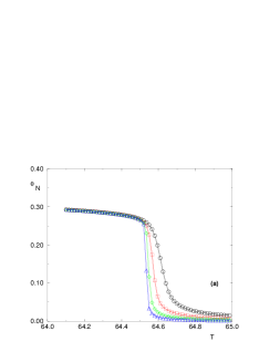
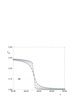
Figure 2: The fraction of paired monomers $\theta_{N}(T)$ of the pure case for sizes $N=10^{5}$ $(\bigcirc)$, $2\cdot 10^{5}$ $(\square)$, $4\cdot 10^{5}$ $(\diamond)$, $8\cdot 10^{5}$ $(\triangle)$. The boundary conditions are (a) bound-bound (b) bound-unbound.

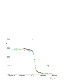
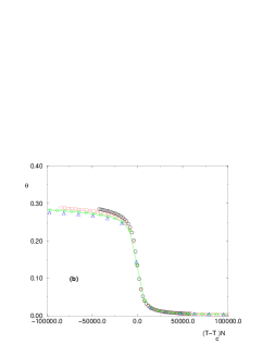
Figure 3: The scaled fraction of paired monomers $\theta((T-T_{c})N)$ of the pure case, for $T_{c}=64.521..$ for sizes $N=10^{5}$ $(\bigcirc)$, $2\cdot 10^{5}$ $(\square)$, $4\cdot 10^{5}$ $(\diamond)$, $8\cdot 10^{5}$ $(\triangle)$. The boundary conditions are (a) bound-bound (b) bound-unbound.

We choose $\varepsilon_{\alpha}=\varepsilon_{0}=-355\ {\rm K}$ (see below). The contact density $\theta_{N}(T)$ defined in eq. (6) is plotted on Fig. 2 for the two boundary conditions (bound-bound) and (bound-unbound) : for the (bb) case, there is no crossing at $T_{c}$ as $N$ varies, whereas for the (bu) case, there is a crossing at $T_{c}\simeq 64.521..$ (Celsius scale), as was also found for the pure SAWs Monte-Carlo simulations (see Fig. 7 of Ref Barbara1 ). From a numerical point of view, the boundary conditions (bu) seem therefore much more interesting since it yields a direct measure of the critical temperature $T_{c}$. With the value of $T_{c}$ obtained from the crossing of Fig. 1 (b), we may now plot on Fig. 2 the contact density $\theta_{N}(T)$ in terms of the rescaled variable $(T-T_{c})N^{\phi}$ with the crossover exponent $\phi=1$ : for the two boundary conditions (bb) and (bu), the finite-size scaling form

$$\theta_{N}(T)=\Theta((T-T_{c})N)$$ (13)

holds in the delocalized phase $T>T_{c}$, as was also found in the pure SAWs Monte-Carlo simulations (see Fig. 7 of Ref Barbara1 ).

III.2 Specific heat

The specific heat is shown on Fig. 4 for the two boundary conditions : in both cases, the maximum $C_{N}^{max}$ scales as the size $N$. For the (bb) case, the temperature $T_{c}(N)$ of the maximum moves towards the critical temperature $T_{c}$ as $T_{c}(N)-T_{c}\sim 1/N$, whereas for the (bu) boundary conditions, the temperature of the maximum remains almost stable as $N$ varies, as was also found in the pure SAWs Monte-Carlo simulations (see Fig. 8 of Ref Barbara1 ).

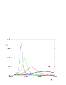
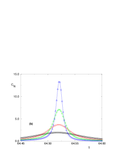
Figure 4: The specific heat $C_{N}$ of the pure case, for sizes $N=10^{5}$ $(\bigcirc)$, $2\cdot 10^{5}$ $(\square)$, $4\cdot 10^{5}$ $(\diamond)$, $8\cdot 10^{5}$ $(\triangle)$. The boundary conditions are (a) bound-bound (b) bound-unbound.

III.3 Pairing probabilities along the chain

On Fig. 5 (a), we have plotted the unpairing probability $q(\alpha)=1-p(\alpha)$ (see eq. 5) as a function of the monomer index $\alpha$, at criticality, for both boundary conditions : for the (bb) boundary condition, this unpairing probability is flat around the value $q_{c}$, whereas for the (bu) boundary condition, the unpairing probability varies linearly as

$$q(\alpha)\simeq q_{c}+(1-q_{c})\frac{\alpha}{N}$$ (14)

This linear behavior actually means that there exists a phase coexistence at $T_{c}$ between the localized phase on $(1,\alpha_{d})$ and the delocalized phase on $(\alpha_{d},N)$, where the position $\alpha_{d}$ of the interface is uniformly distributed on $(1,N)$. In the SAWs simulations, this coexistence with a uniform position of the interface is seen via the flat histogram of the contact density over Monte-Carlo configurations (see Fig. 5 of Ref Barbara1 ). For the (bb) boundary condition, there is no phase coexistence : the whole sample is in the localized phase.

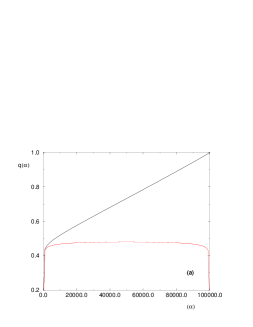
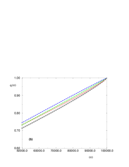
Figure 5: (a) The unpairing probability $q(\alpha)=(1-p(\alpha))$ of the bound-bound (lower curve) and bound-unbound (upper curve) pure case at $T_{c}$, for $N=10^{5}$ and $c_{1}=0$ (b) The unpairing probability $q(\alpha$), $\alpha>\frac{N}{2}$, of various (bu) pure cases at $T_{c}$ for $N=10^{5}$: $c_{1}=0$ ($\triangle$), $c_{1}=0.1$ ($\bigcirc$), $c_{1}=-0.07$ ($\star$), and the prescription of reference Schaf ($\square$). Note that the latter is very close to the case $c_{1}=0$ studied in this paper.

For the (bu) boundary condition, the presence of a free end of length $l\sim N$ at criticality means that the choice of the function $g(\alpha;N)$ in the free end weight of eq. (4) may have some importance for phase coexistence properties at criticality.

A plausible choice, that we have adopted here, is to extend the equation $g(\alpha;N)=\frac{1}{(N-\alpha)^{c_{1}}}$, valid for $(N-\alpha)\ll N$ to all values of $\alpha$. We show in Fig 5 (b) the unpairing probability $q(\alpha)$ for various values of $c_{1}$ : $c_{1}\simeq 0.1$ Ka_Mu_Pe2 and $c_{1}=0$.

Other choices of the exponent $c_{1}$ and/or of the function $g(\alpha;N)$ are possible Baiesi1 ; Schaf ; Schafetal . We show in particular in Fig 5 (b) the unpairing probability $q(\alpha)$ for (i) the value $c_{1}=-0.07$, obtained in ref. Schafetal for a three arm star polymer (ii) the prescription $g(\alpha;N)=\frac{1}{\alpha^{c_{1}}}\frac{1}{(N-\alpha)^{c_{1}}}$, with $c_{1}\simeq 0.1$ advocated in ref Schaf .

As shown in Fig, 5, we obtain only slight deviations with respect to the straight line behavior of eq. (14) obtained for our choice $g(\alpha;N)=\frac{1}{(N-\alpha)^{c_{1}}}$, $c_{1}=0$.

III.4 Conclusion on the pure case

We have shown how the two boundary conditions (bb) and (bu) lead to different behaviors : at criticality, the (bb) case presents a pure localized phase, whereas the (bu) case gives rise to a phase coexistence between a localized phase and a delocalized phase, with an interface uniformly distributed over the sample. In this respect, the (bb) case seems simpler. However, from the point of view of finite size scaling analysis, the (bu) case has the advantage of allowing a direct measure of the critical temperature via the crossing of the contact density.

We have also mentioned how the the presents results for the (bu) case can be qualitatively compared with the pure SAWs simulations Barbara1 , and we refer to Schaf for a detailed quantitative comparison between the two models.

We now turn to the study of the disordered case.

IV Finite size properties of the disordered case

We consider the case of binary disorder where the binding energies $\varepsilon_{\alpha}$ are independent random variables: $\varepsilon_{\alpha}=\varepsilon_{0}=-355\ {\rm K}$ with probability $\frac{1}{2}$ and $\varepsilon_{\alpha}=\varepsilon_{1}=-390\ {\rm K}$ with probability $\frac{1}{2}$. As mentioned in the Introduction, this distribution represent AT and GC base pairs, and the values of ($\varepsilon_{0},\varepsilon_{1}$) are such that the critical temperatures of the pure cases are close to the AT and GC experimental ones.

Disordered averaged quantities $A$ will be denoted by $\overline{A}$.

IV.1 Disordered averaged contact and energy densities

We have plotted on Fig. 6 the disorder averaged contact density $\overline{\theta}_{N}(T)$ for the two boundary conditions : the results are very similar to the pure case results of Fig. 2. In particular, for the (bu) case, the crossing of the contact density for different values of $N$ gives a direct determination of $T_{c}$, and shows that the contact density is finite at criticality: the transition is therefore first order. We also show in Fig. 7 (b) the contact energy of eq. (7) for the (bu) case, which is somewhat similar to the corresponding result for SAW’s (see Fig 4 of ref Barbara2 ). The crossing is again a clear sign of a discontinuous transition.

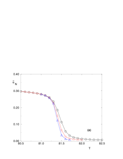
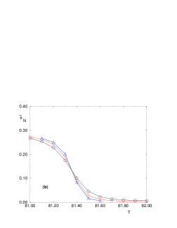
Figure 6: The fraction of paired monomers $\overline{\theta}_{N}(T)$ of the disordered case for sizes $N=10^{5}$ $(\bigcirc)$, $2\cdot 10^{5}$ $(\square)$, $4\cdot 10^{5}$ $(\triangle)$, averaged over $10^{4}$ samples. The boundary conditions are (a) bound-bound (b) bound-unbound. The error bars are much smaller than the symbols.

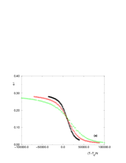
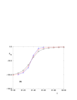
Figure 7: (a) Tentative rescaling $\overline{\theta}_{N}(T)=\Theta((T-T_{c})N)$ for the fraction of paired monomers, averaged over $500$ samples, for sizes $N=10^{5}$ $(\bigcirc)$, $2\cdot 10^{5}$ $(\square)$, $4\cdot 10^{5}$ $(\triangle)$. The boundary condition is bound-bound (b) The contact energy $\overline{e}_{N}(T)$ of the disordered case for sizes $N=10^{5}$ $(\bigcirc)$, $2\cdot 10^{5}$ $(\square)$, $4\cdot 10^{5}$ $(\triangle)$, averaged over $10^{4}$ samples. The boundary condition is bound-unbound. The error bars are much smaller than the symbols.

However, in contrast with the pure case, the rescaling (13) shown on Fig. 7 (a), is not satisfied at all

$$\overline{\theta}_{N}(T)\neq\Theta((T-T_{c})N)$$ (15)

Since the crossing of the contact density of Fig. 6 (b) implies that the transition is first-order, we are led to the conclusion that there is a problem with the finite-size scaling form for the disorder averaged contact density (15). To understand why, we have studied the sample-to-sample fluctuations.

IV.2 Sample to sample fluctuations

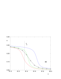
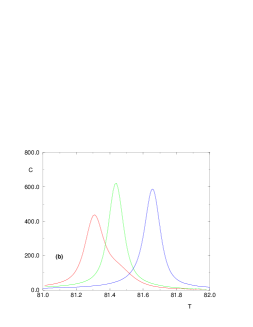
Figure 8: (a) Comparison of the fraction of paired monomers of three individual disorder samples with the average over $10^{4}$ samples $(\bigcirc)$, for size $N=10^{5}$ and bound-bound boundary condition. The thermodynamic critical temperature $T_{c}$ is shown (b) The specific heat of the three disorder samples.

On Fig. 8 (a), we have plotted the contact density for three particular samples, as compared to the average over $10^{4}$ samples. The sample to sample fluctuations are still strong even for the size $N=10^{5}$. In particular, at the critical temperature $T_{c}$ obtained from the crossing of Fig. 6 (b), some samples are clearly already ‘delocalized’, whereas other remain localized up to a higher temperature. On Fig. 8 (b), we have plotted the specific heat for the three same samples : the peaks are clearly separated.

These results are reminiscent of the lack of self-averaging found in second order random critical points domany95 ; domany . In these systems, the argument goes as follows domany (i) off-criticality, the finite correlation length $\xi$ allows for a division of the sample into independent large sub-samples, which in turn leads to the self-averaging property of thermodynamic quantities (here, “independent” means that that the interaction term between these sub-samples is a surface term, that can be neglected with respect to volume contributions) (ii) at criticality however, the previous ’subdivision’ argument breaks down because of the divergence of $\xi$.

In usual first-order transitions, there is no diverging correlation length. The analysis of the disorder effects consists in dividing the system into finite sub-systems (or phases), and in taking into account the surface tension between phases Im_Wo . The first order transition of the PS model is very different for two polymeric reasons. First, there is no surface tension between the localized and delocalized phases, as explained in section III.3 on the coexistence at the pure critical point. Second, there exists here an infinite correlation length, as is very clear in the (bu) case where the end segment length diverges as $1/(T_{c}-T)$ Ka_Mu_Pe2 . In the (bb) case, this diverging correlation length appears in the loop length distribution

$$P_{T}^{pure}(l)\simeq\frac{1}{l^{c}}\ e^{-\frac{l}{\xi(T)}}\ \ \ {\rm with}\ \ \xi(T)\mathop{\simeq}_{T\to T_{c}^{-}}\frac{1}{T_{c}-T}\$$ (16)

We are therefore led to the conclusion that the lack of self-averaging we find in the disordered PS model comes from the presence of an infinite correlation length, (even though the transition is first order), that prevents the division of the chain into independent sub-chains.

The strong sample-to sample fluctuations explain why the finite-size scaling analysis (15) does not work for the disordered averaged contact density : each sample $(i)$ has its own pseudo-critical temperature $T_{c}(i)$ where it presents a pseudo-first order transition, and the resulting disorder average has no nice finite-size scaling behavior.

IV.3 Finite-size scaling for the contact density in a given sample

Since we have obtained that there are strong sample to sample fluctuations that invalidates the usual finite size scaling analysis for the disorder averaged contact density, we have tried to use more refined finite size scaling theories in the presence of disorder domany95 ; Paz1 ; domany ; Paz2 : in these references, it is stressed that the sample to sample fluctuations of a given observable are predominantly due to the sample to sample fluctuations of the pseudo-critical temperatures $T_{c}(i,N)$. As a consequence, these references express the finite size scaling form of an observable $X$ domany ; Paz2 as

$$X_{N}^{(i)}(T)=N^{\rho}Q_{i}\left((T-T_{c}(i,N))N^{\phi}\right)$$ (17)

where $T_{c}(i,N)$ is the pseudo-critical temperature of the sample $i$, determined for instance as the susceptibility peak domany , or by a minimal distance criterium Paz2 . The scaling function $Q_{i}$ a priori also depends on the sample, and we refer to domany ; Paz2 for discussions and examples.

Here, from the specific heat plotted on Fig 8b, we see that beyond the sample dependence of the pseudo-critical temperature $T_{c}(i)$, there is also a sample dependent scaling function $Q_{i}$, in contrast with the case studied in Paz2 , where the curves of various samples were the same up to a translation $T-T_{c}(i)$.

As a consequence, we have tried to obtain some information from a sample-dependent finite-size scaling analysis via the following ’sample replication’ procedure : we have compared a given random sample $E=(\epsilon_{1},...,\epsilon_{N})$ of size $N=10^{5}$ with the sample of size $2N=2.10^{5}$ obtained by gluing together two copies of the initial sample $E$, and with the sample of size $4N=4.10^{5}$ obtained by gluing together four copies of the initial sample $E$ : the corresponding results for the contact density for the two boundary conditions are shown on Fig. 9. In particular, the crossing obtained for the (bu) boundary conditions allows to determine the sample-dependent pseudo-critical temperature $T_{c}(i)$. The rescaling of these data with the reduced variable $x=(T-T_{c}(i))N$ is found to be satisfactory in the delocalized phase $T>T_{c}(i)$ for the two boundary conditions, see Fig. 10. We have also plotted on Fig. 11 the associated specific heats : for the two boundary conditions, the maximum value scales as $N$.

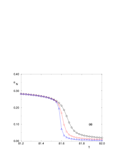
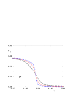
Figure 9: The fraction of paired monomers $\theta_{N}(T)$ for a single disorder sample, using the ’sample replication’ procedure discussed in the text, and for sizes $N=10^{5}$ $(\bigcirc)$, $2\cdot 10^{5}$ $(\square)$, $4\cdot 10^{5}$ $(\triangle)$. The boundary conditions are (a) bound-bound (b) bound-unbound.

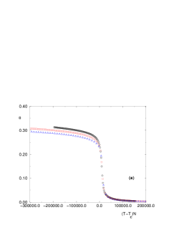
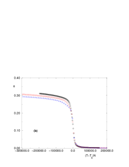
Figure 10: The scaled fraction of paired monomers $\theta((T-T_{c})N))$ for the same disorder sample as in Fig 9, for sizes $N=10^{5}$ $(\bigcirc)$, $2\cdot 10^{5}$ $(\square)$, $4\cdot 10^{5}$ $(\triangle)$. The boundary conditions are (a) bound-bound (b) bound-unbound.

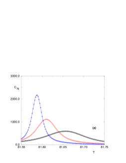
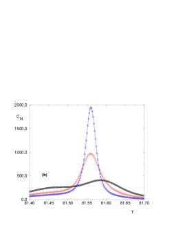
Figure 11: The specific heat $C_{N}$ for the same disorder sample as in Fig 9 and Fig 10, for sizes $N=10^{5}$ $(\bigcirc)$, $2\cdot 10^{5}$ $(\square)$, $4\cdot 10^{5}$ $(\triangle)$. The boundary conditions are (a) bound-bound (b) bound-unbound.

IV.4 Pairing probability along the chain in a given sample

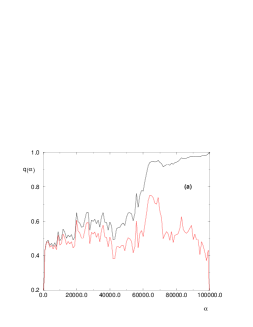
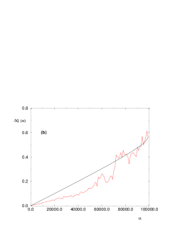
Figure 12: (a) The unpairing probability $q(\alpha)$ for a single disorder sample $(i)$ at its critical temperature $T_{c}(i)$, for size $N=10^{5}$. The boundary conditions are bound-bound (lower curve) and bound-unbound (upper curve)(b) The difference $\Delta q(\alpha)=q_{bu}(\alpha)-q_{bb}(\alpha)$ between the two previous curves compared with the analog quantity of the pure case at $T_{c}$ (see Figure 5 (a)).

On Fig. 12(a), we have plotted, for a given sample at its pseudo-critical temperature $T_{c}(i)$ determined by Fig. 9 (b), the unpairing probability $q(\alpha)$ as a function of the monomer index $\alpha$ for the two boundary conditions. These data should be compared with the pure case results of Fig. 5 : beside the disorder fluctuations present in the (bb) boundary conditions, the (bu) boundary conditions display an upward trend that shows that there exists some phase coexistence between a localized and delocalized phase. To show more clearly this coexistence, we have plotted in Fig. 12(b) the difference $\Delta q(\alpha)=q_{bu}(\alpha)-q_{bb}(\alpha)$ for the same disordered sample, as compared to the linear analog of the pure case.

IV.5 Disorder averaged loop statistics

We now turn to the probability measure $M_{N}(l)$ of the loops of length $l$ existing in a sample of size $N$, as defined in eq. (9). In Fig. 13, we present the disorder averaged $\overline{M_{N}(l)}$ at criticality, in terms of the rescaled length $\lambda=l/N$ for the two boundary conditions (bb) and (bu). In each case, we have added the corresponding pure critical analog for comparison.

In the pure case, the loop length distribution at criticality is given in the thermodynamic limit by the loop weight used to defined the PS model (2) $P(l)\sim 1/l^{c}$. Here in the pure finite sample, the exponent $c=2.15$ indeed corresponds to the slope in the regime $l\ll N$, before the appearance of some curvature near $l\sim N$. This form for the pure critical loop statistics is thus very similar to the corresponding result for pure SAWs Carlon ; Baiesi1 ; Baiesi2 . In the disordered case, we clearly obtain the same slope $c=2.15$ in the regime $l\ll N$, and deviations with respect to the pure case only occur in the region $l\sim N$. Our conclusion is thus that in the presence of disorder, the statistics of loops at criticality remains $P(l)\sim 1/l^{c}$ in the thermodynamic limit as in the pure case.

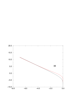
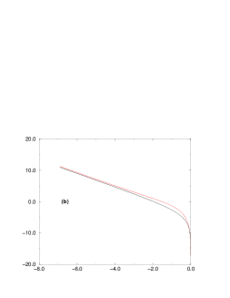
Figure 13: Log-Log plot of the critical loop distribution $M_{N}(l)$ in the rescaled variable $\lambda=\frac{l}{N}$ for the disordered case (averaged over $10^{4}$ samples) and for the pure case (lower curve). Both systems have size $N=10^{5}$ and the boundary conditions are (a) bound-bound (b) bound-unbound.

V Conclusion

In this paper, we have studied the binary disordered Poland-Scheraga model of DNA denaturation, in the regime where the pure model displays a first order transition (loop exponent $c>2$). Our main conclusion is that the transition remains first order in the disordered case, but that disorder averaged observables do not satisfy finite size scaling, as a consequence of strong sample to sample fluctuations.

Let us now consider the relation between the PS model and the Monte Carlo simulations of attracting SAW’s. In the pure case, the finite-size behavior we have presented for the PS model with (bu) boundary conditions is very similar to the corresponding behavior obtained previously in Monte-Carlo simulations of SAW’s Barbara1 . In the disordered case, our result for the crossing of the contact energy (Fig 7 (b)) is somewhat similar to the corresponding results (Fig 4) of ref. Barbara2 . The failure of finite size scaling for disordered averaged quantities was also noted in this reference. It therefore seems that the PS model with (bu) boundary conditions is an appropriate effective model for SAW’s even in the presence of disorder.

Acknowledgments : We are grateful to B. Coluzzi for communicating her results Barbara2 on disordered SAWs prior to publication: they motivated the present study on the PS model. We thank Y. Kafri and H. Orland for discussions.

References

- (1) M.S. Causo, B. Coluzzi and P. Grassberger Phys. Rev. E 62, 3958 (2000)
- (2) E. Carlon, E. Orlandini and A.L. Stella, Phys. Rev. Lett., 88, 198101 (2002).
- (3) M. Baiesi, E. Carlon, and A.L. Stella, Phys. Rev. E, 66, 021804 (2002).
- (4) M. Baiesi, E. Carlon, Y. Kafri, D. Mukamel, E. Orlandini and A.L. Stella, Phys. Rev. E, 67, 021911 (2002).
- (5) Y. Kafri, D. Mukamel and L. Peliti, Phys. Rev. Lett., 85, 4988 (2000).
- (6) Y. Kafri, D. Mukamel and L. Peliti, Eur. Phys. J. B, 27, 135 (2002).
- (7) C. Richard and A. J. Guttmann, J. Stat. Phys., 115, 943 (2004).
- (8) L. Schäfer, cond-mat 0502668.
- (9) D. Poland and H.A. Scheraga eds., Theory of Helix-Coil transition in Biopolymers, Academic Press, New York (1970).
- (10) M.E. Fisher, J, Chem. Phys., 45, 1469 (1966).
- (11) B. Duplantier, Phys. Rev. Lett., 57, 941 (1986); J. Stat. Phys., 54, 581 (1989).
- (12) B. Coluzzi, cond-mat/0504080.
- (13) Y. Imry and M. Wortis, Phys. Rev. B, 19, 3580 (1979)
- (14) M. Aizenman and J, Wehr, Phys. Rev, Lett., 62, 2503 (1989); (E) 64, 1311 (1990)
- (15) K. Hui and A.N. Berker, Phys. Rev, Lett., 62, 2507 (1989)
- (16) J. Cardy, Physica A, 263, 215 (1999)
- (17) T. Garel and C. Monthus, cond-mat 0502195
- (18) R.M. Wartell and A.S. Benight, Phys. Repts., 126, 67 (1985).
- (19) R.D. Blake, J.W. Bizarro, J.D. Blake, G.R. Day, S.G. Delcourt, J. Knowles, K.A. Marx and J. SantaLucia Jr., Bioinformatics, 15, 370-375 (1999); see also J. Santalucia Jr., Proc. Natl. Acad. Sci. USA, 95, 1460 (1998).
- (20) T. Garel and H. Orland, Biopolymers, 75, 453 (2004).
- (21) P.G. de Gennes, Scaling concepts in polymer physics, Cornell University Press, Ithaca, (1979).
- (22) M. Fixman and J.J. Freire, Biopolymers, 16, 2693 (1977)
- (23) E. Yeramian, Genes, 255, 139, 151 (2000).
- (24) L. Schäfer, C. von Ferber, U. Lehr and B. Duplantier, Nuclear Phys. B, 374, 473 (1992).
- (25) S. Wiseman and E. Domany, Phys Rev E 52, 3469 (1995).
- (26) F. Pázmándi, R.T. Scalettar and G.T. Zimányi, Phys. Rev. Lett. 79, 5130 (1997).
- (27) S. Wiseman and E. Domany, Phys. Rev. Lett. 81, 22 (1998) ; Phys Rev E 58, 2938 (1998).
- (28) K. Bernardet, F. Pázmándi and G.G. Batrouni, Phys. Rev. Lett. 80, 4477 (2000).