Real-time dynamics at finite temperature by DMRG:
A path-integral approach

Abstract

We propose a path-integral variant of the DMRG method to calculate real-time correlation functions at arbitrary finite temperatures. To illustrate the method we study the longitudinal autocorrelation function of the $XXZ$-chain. By comparison with exact results at the free fermion point we show that our method yields accurate results up to a limiting time which is determined by the spectrum of the reduced density matrix.

The density-matrix renormalization group (DMRG) White (1992) is today a well established numerical method to study ground state properties of one-dimensional quantum systems. Within the last few years the DMRG method has been generalized to allow also for the calculation of spectral functions Jeckelmann (2002) and, quite recently, to incorporate directly real-time evolution.White and Feiguin (2004) The most powerful variant of DMRG to calculate thermodynamic properties is the density-matrix renormalization group applied to transfer matrices (TMRG). This method has been proposed by Bursill et al. Bursill et al. (1996) and has later been improved considerably.Wang and Xiang (1997) The main idea of TMRG is to express the partition function $Z$ of a one-dimensional quantum model by that of an equivalent two-dimensional classical model obtained by a Trotter-Suzuki decomposition.Trotter (1959) Thermodynamic quantities can then be calculated by considering a suitable transfer matrix $\mathcal{T}$ for the classical model. The main advantage of this method is that the thermodynamic limit (chain length $L\rightarrow\infty$) can be performed exactly and that the free energy in the thermodynamic limit is determined solely by the largest eigenvalue of $\mathcal{T}$. The TMRG has been applied to calculate static thermodynamic properties for a variety of one-dimensional systems including spin chains, the Kondo lattice model, the $t-J$ chain and ladder, and also spin-orbital models.Eggert and Rommer (1998); Mutou et al. (1998); Sirker and Klümper (2002b)

The Trotter-Suzuki decomposition of a one-dimensional quantum system yields a two-dimensional classical model with one axis corresponding to imaginary time (inverse temperature). It is therefore straightforward to calculate imaginary-time correlation functions (CFs) using the TMRG algorithm. Although the results for the imaginary-time CFs obtained by TMRG are very accurate, the results for real-times (real-frequencies) involve large errors because the analytical continuation poses an ill-conditioned problem. In practice it has turned out that the maximum entropy method is the most efficient and reliable way to obtain spectral functions from TMRG data. The combination of TMRG and maximum entropy has been used to calculate spectral functions for the $XXZ$-chain Naef et al. (1999) and the Kondo-lattice model.Mutou et al. (1998) However, this method involves intrinsic errors due to the analytical continuation which cannot be resolved.

Here we propose a method to calculate directly real-time CFs at finite temperature by a modified TMRG algorithm thus avoiding an analytical continuation. We start by considering the two-point CF for an operator $\hat{O}_{r}(t)$ at site $r$ and time $t$

$$\langle\hat{O}_{r}(t)\hat{O}_{0}(0)\rangle = \frac{\mbox{Tr}\left(\hat{O}_{r}(t)\hat{O}_{0}(0)\text{e}^{-\beta H}\right)}{\mbox{Tr}\left(\text{e}^{-\beta H}\right)}$$

$$= \frac{\mbox{Tr}\left(\text{e}^{-\beta H/2}\text{e}^{\text{i}tH}\hat{O}_{r}\text{e}^{-\text{i}tH}\hat{O}_{0}\text{e}^{-\beta H/2}\right)}{\mbox{Tr}\left(\text{e}^{\text{i}tH}\text{e}^{-\text{i}tH}\text{e}^{-\beta H}\right)}\;$$

where $\beta$ is the inverse temperature. Here we have used the cyclic invariance of the trace and have written the denominator in analogy to the numerator. For a Hamiltonian $H$ with nearest-neighbor interactions we can use the Trotter-Suzuki decomposition

$$\text{e}^{-\epsilon H}=\text{e}^{-\epsilon H_{odd}/2}\text{e}^{-\epsilon H_{even}}\text{e}^{-\epsilon H_{odd}/2}+\mathcal{O}(\epsilon^{3})$$ (2)

where $\epsilon=\beta/M$ so that the partition function $Z=\exp(-\beta H)$ becomes

$$Z=\text{Tr}\left(\prod_{i=\text{odd}}\text{e}^{-\epsilon h_{i,i+1}}\prod_{i=\text{even}}\text{e}^{-\epsilon h_{i,i+1}}\right)^{M}\left(1+\mathcal{O}(\epsilon^{2})\right)\;.$$ (3)

With $\text{i}t\rightarrow\tau$ in Eq. (Real-time dynamics at finite temperature by DMRG: A path-integral approach) and inserting the identity operator at each imaginary time step one obtains directly a lattice path-integral representation for the imaginary time CF $\langle\hat{O}_{r}(\tau)\hat{O}_{0}(0)\rangle$.Naef et al. (1999); Mutou et al. (1998)

The crucial step in our new approach for real times is to introduce a second Trotter-Suzuki decomposition of $\exp(-\text{i}\delta H)$ as in Eq. (2) with $\delta=t/N$. We can then define a column-to-column transfer matrix

$$\mathcal{T}_{2N,M} = (\tau_{1,2}\tau_{3,4}\cdots\tau_{2M-1,2M})(\tau_{2,3}\tau_{4,5}\cdots\tau_{2M,2M+1})$$ (4)

$$(\bar{v}_{2M+1,2M+2}\cdots\bar{v}_{2M+2N-1,2M+2N})$$

$$(\bar{v}_{2M+2,2M+3}\cdots\bar{v}_{2M+2N,2M+2N+1})$$

$$(v_{2M+2N+1,2M+2N+2}\cdots v_{2M+4N-1,2M+4N})$$

$$(v_{2M+2N+2,2M+2N+3}\cdots v_{2M+4N,1})$$

where the local transfer matrices have matrix elements

$$\tau(s_{k}^{i}s_{k}^{i+1}|s_{k+1}^{i}s_{k+1}^{i+1}) = \langle s_{k}^{i}s_{k}^{i+1}|\text{e}^{-\epsilon h_{i,i+1}}|s_{k+1}^{i}s_{k+1}^{i+1}\rangle$$ (5)

$$v(s_{l}^{i}s_{l}^{i+1}|s_{l+1}^{i}s_{l+1}^{i+1}) = \langle s_{l}^{i}s_{l}^{i+1}|\text{e}^{-\text{i}\delta h_{i,i+1}}|s_{l+1}^{i}s_{l+1}^{i+1}\rangle\;$$

and $\bar{v}$ is the complex conjugate. Here $i=1,\cdots,L$ is the lattice site, $k=1,\cdots,2M$ ($l=1,\cdots,2N$) the index of the imaginary time (real time) slices and $s_{k(l)}^{i}$ denotes a local basis. The denominator in Eq. (Real-time dynamics at finite temperature by DMRG: A path-integral approach) can then be represented by $\mbox{Tr}(\mathcal{T}_{2N,M}^{L/2})$ where $N,M,L\rightarrow\infty$. A similar path-integral representation holds for the numerator in (Real-time dynamics at finite temperature by DMRG: A path-integral approach). Here we have to introduce an additional modified transfer matrix $\mathcal{T}_{2N,M}(\hat{O})$ which contains the operator $\hat{O}$ at the appropriate position. For $r>1$ we find

$$\langle\hat{O}_{r}(t)\hat{O}_{0}(0)\rangle$$

$$=\lim_{N,M\rightarrow\infty}\lim_{L\rightarrow\infty}\frac{\mbox{Tr}(\mathcal{T}(\hat{O})\mathcal{T}^{[r/2]-1}\mathcal{T}(\hat{O})\mathcal{T}^{L/2-[r/2]-1})}{\mbox{Tr}(\mathcal{T}^{L/2})}$$

$$=\lim_{N,M\rightarrow\infty}\frac{\langle\Psi^{L}_{0}|\mathcal{T}(\hat{O})\mathcal{T}^{[r/2]-1}\mathcal{T}(\hat{O})|\Psi^{R}_{0}\rangle}{\Lambda_{0}^{[r/2]+1}\langle\Psi^{L}_{0}|\Psi^{R}_{0}\rangle}\;.$$ (6)

Here $[r/2]$ denotes the first integer smaller than or equal to $r/2$ and we have set $\mathcal{T}\equiv\mathcal{T}_{2N,M}$. In the second step we have used the fact that the spectrum of the column-to-column transfer matrix $\mathcal{T}$ is gapped for $\beta<\infty$.Wang and Xiang (1997) Therefore the trace is reduced to an expectation value where $|\Psi^{R}_{0}\rangle,\langle\Psi^{L}_{0}|$ are the right- and left-eigenvectors of the non-hermitian transfer matrix $\mathcal{T}$ belonging to the largest eigenvalue $\Lambda_{0}$. A graphical representation of the transfer matrices appearing in the numerator of Eq. (Real-time dynamics at finite temperature by DMRG: A path-integral approach) is shown in Fig. 1.

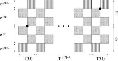
Figure 1: Transfer matrices appearing in the numerator of Eq. (Real-time dynamics at finite temperature by DMRG: A path-integral approach) for $r>1$ with $r$ even. The 2 black dots denote the operator $\mathcal{O}$. Each transfer matrix consists of three parts: A part representing $\exp(-\beta H)$ (vertically striped plaquettes), another for $\exp(\text{i}tH)$ (stripes from lower left to upper right) and a third part describing $\exp(-\text{i}tH)$ (upper left to lower right). The transfer matrices $\mathcal{T},\mathcal{T}(O)$ are split into a system (S) and an environment block (E).

It is worth to note that Eq. (Real-time dynamics at finite temperature by DMRG: A path-integral approach) has the same structure as the equation for the calculation of imaginary time CFs.Naef et al. (1999); Mutou et al. (1998) Only the transfer matrices involved are different. For practical DMRG calculations the parameters $\epsilon,\delta$ are fixed and the temperature (time) is decreased (increased) by increasing M (N). This is achieved by splitting $\mathcal{T},\mathcal{T}(O)$ into a system and an environment block (see Fig. 1). Adding an additional $\tau$-plaquette at the lower end of the system block then decreases the temperature whereas adding a $v$-plaquette at the upper end leads to an increase in time $t$. The extended system block is renormalized by projecting onto the $Z$ largest eigenstates of the reduced density matrix $\rho_{S}=\mbox{Tr}_{E}|\Psi^{R}_{0}\rangle\langle\Psi^{L}_{0}|$. Starting from an existing TMRG program our real-time algorithm requires only the following minor changes: In addition to the $\tau$-plaquettes also $v$-plaquettes are present. Therefore the transfer matrix and the density matrix become complex quantities so that complex diagonalization routines are required.

In the remainder of this letter we want to study, as a highly non-trivial example, the longitudinal autocorrelation $C(t,T)=\langle S^{z}_{0}(t)S^{z}_{0}(0)\rangle$ at temperature $T$ for the $XXZ$ chain with Hamiltonian

$$H=J\sum_{i}\left(S^{x}_{i}S^{x}_{i+1}+S^{y}_{i}S^{y}_{i+1}+\Delta S^{z}_{i}S^{z}_{i+1}\right)$$ (7)

where $S=1/2$, $J>0$ and $\Delta\geq 0$. Although the model is integrable, exact results for $C(t,T)$ are available only at the free fermion point $\Delta=0$. Quite interestingly, $C(t,T)$ shows a non-trivial behavior even at infinite temperature due to the quantum nature of the problem.Fabricius and McCoy (1998)

For the autocorrelation both $S^{z}$ operators are situated in the same transfer matrix $\mathcal{T}(S^{z},S^{z})$ so that Eq. (Real-time dynamics at finite temperature by DMRG: A path-integral approach) reduces to

$$C(t,T)=\frac{\langle\Psi^{L}_{0}|\mathcal{T}(S^{z},S^{z})|\Psi^{R}_{0}\rangle}{\Lambda_{0}\langle\Psi^{L}_{0}|\Psi^{R}_{0}\rangle}\;.$$ (8)

It is important to note that once the blocks necessary to construct $\mathcal{T},\mathcal{T}(S^{z},S^{z})$ at a given time $t$ are known, the correlation function for arbitrary distance $r$ with $t$ fixed can be simply calculated by additional matrix-vector multiplications (see Eq. (Real-time dynamics at finite temperature by DMRG: A path-integral approach)). We start with the case $T=\infty$ where $\mathcal{T},\mathcal{T}(S^{z},S^{z})$ do not contain any $\tau$-plaquettes. This limit directly addresses the essential feature in our approach, namely the transfer-matrix representation of the time evolution operator. In Fig. 2 results for $\Delta=0$ and $\Delta=1$ are shown where the number of states kept in the DMRG varies between $Z=50$ and $Z=400$.

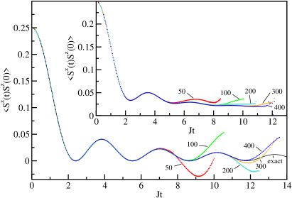
Figure 2: Longitudinal autocorrelation for $\Delta=0$ and $\Delta=1$ (inset) at $T=\infty$ where the number of states kept varies between $Z=50$ and $400$ and $\delta=0.1$. The exact result is shown for comparison in the case $\Delta=0$.

In the case $\Delta=0$ the autocorrelation function can be calculated exactly by mapping the system to a free spinless fermion model using the Jordan-Wigner transformation. For arbitrary temperature $T$ the result can be expressed as $C(t,T)=\{D_{1}(t)+D_{2}(t,T)\}^{2}$ with

$$D_{1}(t)=\frac{J_{0}(Jt)}{2}\;,\;D_{2}(t,T)=\frac{\text{i}}{\pi}\int_{0}^{1}\frac{\sin J\theta t}{\sqrt{1-\theta^{2}}}\tanh\frac{\theta}{2T}d\theta$$ (9)

where $J_{0}$ is the Bessel function of order zero.Niemeijer (1967) At $T=\infty$ this reduces to $C(t,\infty)=J_{0}^{2}(Jt)/4$. Our numerical results agree with the exact one up to a maximum time which is determined by the number of states kept in the DMRG. For the maximum number of states, $Z=400$, considered here we are able to reproduce the exact result up to $Jt\sim 12$. For $\Delta=1$ no exact result is available to compare with, however, the $\Delta=0$ case suggests that the results are trustworthy at least as long as they agree with the data where a much smaller number of states is kept. The numerical data with $Z=400$ should therefore be correct at least up to $Jt\sim 10$. We also checked the $\Delta=1$ data for small $t$ by comparing with exact diagonalization. For TMRG calculations the free fermion point is in no way special and the algorithm is expected to show the same behavior at this point as for general $\Delta$.Sirker and Klümper (2002b) In the following we will therefore concentrate on $\Delta=0$ where a direct comparison with exact results is possible.

For small $t$ the error in the numerics is entirely dominated by the finite Trotter-Suzuki decomposition parameter $\delta$. It is therefore possible to enhance the accuracy by decreasing $\delta$ as shown in Fig. 3(a). As expected, the error is quadratic in $\delta$ but fortunately with a rather small pre-factor $\sim 10^{-3}$. For small $\delta$ more RG steps are necessary to reach the same $t$. Interestingly, the breakdown of the algorithm does not depend on the number of RG steps. For different $\delta$ but fixed $Z$ it always occurs at about the same time $t_{c}$. Furthermore the breakdown is always a very rapid one, i.e., for times considerably larger than $t_{c}$ the errors become arbitrarily large. This suggests that there is an intrinsic maximum time scale set by the problem itself. This is supported by Fig. 3(b) showing a rapid increase in the number of states $Z_{n}$ necessary to keep the error below $10^{-3}$.

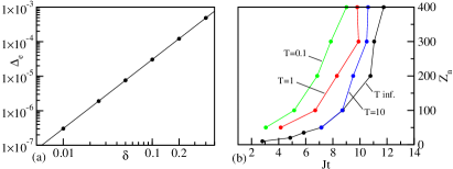
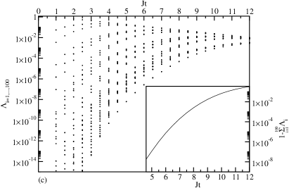
Figure 3: (a) $\Delta_{e}=|C(t,\infty)_{exact}-C(t,\infty)_{TMRG}|$ at $t=4$ as a function of $\delta$ with $Z=100$ states kept. The line corresponds to a fit with $\Delta_{e}=3.05\cdot 10^{-3}\delta^{2}$. (b) Number of states $Z_{n}$ required to keep the error below $10^{-3}$ as function of $t$ for $T/J=\infty,10,1,0.1$. (c) Largest 100 eigenvalues $\Lambda_{i}$ of $\rho_{S}$ at $T=\infty$ calculated exactly. The inset shows the discarded weight $1-\sum_{i=1}^{100}\Lambda_{i}$.

To understand this behavior we have calculated the spectrum of the reduced density matrix $\rho_{S}$ exactly for $T=\infty$ and $\Delta=0$. The result is shown in Fig. 3(c). For small $t$ the spectrum is decaying rapidly so that indeed a few states are sufficient to represent the transfer matrix $\mathcal{T}$ accurately. At larger time scales, however, the spectrum becomes dense. This means that the number of states needed for an accurate representation starts to increase exponentially in agreement with our numerical findings shown in Fig.3(b). The breakdown approximately occurs when the discarded weight defined by $1-\sum_{i=1}^{Z}\Lambda_{i}$, where $\Lambda_{i}$ are the $Z$ largest eigenvalues of $\rho_{S}$, becomes larger than $10^{-3}$ (see inset of Fig. 3(c)). The long-time asymptotics of the autocorrelation function at $T=\infty$ is therefore not accessible within our method.

Next, we consider finite temperatures $0<T<\infty$. Results for $\Delta=0$ and $T/J=10,1,0.1$ are shown in Fig. 4. According to Eq. (9), $C(t,T)$ now acquires also an imaginary part which is shown in the insets of Fig. 4.

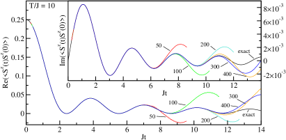
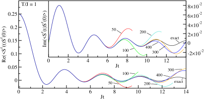
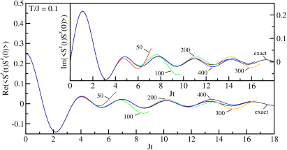
Figure 4: $C(t,T)$ for $\Delta=0$ at $T/J=10,1,0.1$. The main figures show the real, the insets the imaginary parts.

For $T/J=10$ and $T/J=1$ the results look qualitatively similar to the $T=\infty$ case. As shown in Fig. 3(b) the number of states needed to obtain the same accuracy at a given time increases with decreasing temperature. This is easy to understand because the Hilbert space for $\mathcal{T}$ increases when adding additional $\tau$-plaquettes. The breakdown of the algorithm also looks similar to the $T=\infty$ case and we again find an exponential increase in $Z_{n}$ at larger times. As we have chosen $\epsilon=\delta$, the number of $\tau$-plaquettes $M$ is much smaller than the number of $v$-plaquettes $N$ for $t\sim 10$ where the calculations with $Z=300,400$ states fail. The spectrum of the reduced density matrix $\rho_{S}$ at these time scales will therefore look very similar to the one for $T=\infty$ shown in Fig. 3(c). We therefore conclude that it is again the spectrum of $\rho_{S}$ which sets the limiting time for our calculations.

For $T/J=0.1$, however, we find a different behavior. Instead of a rapid breakdown with arbitrarily large deviations for $t>t_{c}$ we find that the results for all $Z$ remain relatively close to the exact one over the entire time scale investigated (the data for $Z=50,100$ in Fig. 4 are depicted only up to times marking the start of deviations). We also see from Fig. 3(b) that the functional form of the increase in $Z_{n}$ is now different from the cases $T/J=\infty,10,1$. Whereas it becomes exponential in the latter, it is more or less linear for $T/J=0.1$ from $Z_{n}=200$ to $Z_{n}=400$. This can be understood as follows: For a transfer matrix $\mathcal{T}$ consisting only of $\tau$-plaquettes, the spectrum of $\rho_{S}$ is exponentially decaying. This characteristic should be preserved as long as the number of $v$-plaquettes is not much larger than the number of $\tau$-plaquettes. A fundamental failure of our approach due to a dense spectrum of $\rho_{S}$ should only occur for $N\gg M$. By considerably increasing $Z$ it should therefore be possible to access much larger time scales at low temperatures in future large scale numerical studies.

To conclude, we have presented a numerical method to calculate real-time correlations in one-dimensional quantum systems at finite temperature. The method is based on a DMRG algorithm applied to transfer matrices. As essentially new ingredient it involves a second Trotter-Suzuki decomposition for the time evolution operator. To test our approach we have calculated the autocorrelation function for the $XXZ$-chain both at infinite and finite temperatures. For $T=\infty$ we have established that reliable results can be obtained up to a maximum time scale $t_{c}$ where the spectrum of the reduced density matrix $\rho_{S}$ becomes dense. For low $T$ we have shown that the algorithm does not show a rapid breakdown contrary to the high-$T$ case and have argued that the fundamental problem of $\rho_{S}$ becoming dense is less severe. A huge advantage of our approach compared to other methods is that once the blocks necessary to construct $\mathcal{T},\mathcal{T}(O)$ at a given time $t$ are known, the CF can be evaluated at time $t$ for arbitrary distances $r$ between the operators $O$ by simple matrix-vector multiplications. As our approach is working directly in the thermodynamic limit it is possible to obtain highly accurate results even for large distances as has been demonstrated for the static case in Ref. Sirker and Klümper, 2002b. This will be exploited in a forthcoming publication Sirker and Klümper (2002c) for a detailed study of time ($t<t_{c}$) and space dependent CFs in the $XXZ$ chain.