Numerical study of a disordered model for DNA denaturation transition

Abstract

We numerically study a disordered version of the model for DNA denaturation transition (DSAW-DNA) consisting of two interacting SAWs in $3d$, which undergoes a first order transition in the homogeneous case. The two possible values ${\hat{\epsilon}_{AT}}$ and ${\hat{\epsilon}_{GC}}$ of the interactions between base pairs are taken as quenched random variables distributed with equal probability along the chain. We measure quantities averaged over disorder such as the energy density, the specific heat and the probability distribution of the loop lengths. When applying the scaling laws used in the homogeneous case we find that the transition seems to be smoother in the presence of disorder, in agreement with general theoretical arguments, although we can not rule out the possibility of a first order transition.

Service de Physique Théorique - CEA - Saclay - Orme des Merisiers 91191 Gif-sur-Yvette cedex, France

PACS: 87.14Gg,87.15.Aa,64.60.Fr,82.39.Pj

1 Introduction

The DNA denaturation transition is an old-standing open problem [1] and one finds in the literature a large number of different models that look in detail at various aspects [2]-[5], for instance reproducing the double-helix structure and the corresponding denaturation behaviour in the whole temperature-torsion plane [4] or taking into account to different extents the role of the stacking energies [3, 5]. From the experimental point of view, one observes a multi-step behaviour in light absorption as a function of temperature which suggests a sudden sharp opening of clusters of base pairs in cooperatively melting regions. Therefore one expects that a theoretical model, correctly reproducing the experimental behaviour, should undergo a sharp transition and there has recently been a lot of interest in models possibly displaying a first order transition in the homogeneous case [4]-[11].

Most programs, for example MELTSIM [12], predict the experimentally observed melting curves using a model originally introduced by Poland and Scheraga [2, 11] that takes into account the different entropic weights of opened loops and double stranded segments. In the first studies of this model, excluded volume effects were completely neglected and a smooth second order transition was predicted in two and three dimensions. By solving the model including the entropic weights of self-avoiding loops [13], one finds a sharper but still second order transition. In this way the self-avoidance between bases within the same loop is taken into account, but other mutual excluded volume effects are still neglected.

In a previous work [7] we pointed out the importance of excluded volume effects between different segments and loops by introducing and numerically studying a model inspired by the former of Poland and Scheraga, consisting of two interacting self-avoiding walks on a $3d$ lattice (SAW-DNA).

In the limit of infinite chain length, the SAW-DNA model undergoes a first order phase transition from the double strand to the molten single-stranded chain state when varying the temperature. The order parameter, which is the energy or the density of binded base pairs, varies abruptly from one to zero.

It has been theoretically demonstrated that the transition in the homogeneous model by Poland and Scheraga is of first order when excluded volume effects are completely taken into account, using the entropic weight of a self-avoiding loop embedded in a self-avoiding chain [8, 14]. This can be obtained as a particular case of a more general result on polymer networks [15]. It has also been analytically shown that only considering the self-avoidance between the two different chains leads to a first order transition [10, 16].

Moreover, several numerical investigations [9, 16, 17, 18] of the homogeneous SAW-DNA model carefully measured the probability distribution of the lengths of denatured loops $P(l)$ at the critical point in $3d$ and $2d$. These confirmed the theoretically expected power law $P(l)\propto 1/l^{c}$ with exponent $c>2$ (in agreement with the transition being first order) in both dimensions.

In the same SAW-DNA model, a first order unzipping transition is predicted in the presence of an external force that pulls apart the two DNA strands [14]. The behaviour in the temperature-force plane is numerically investigated in [19], and a phase diagram with a re-entrance region is observed.

The version of the Poland-Scheraga model on which programs for predicting experimental denaturation curves are based, contains another main parameter, the cooperativity factor $\sigma$, which takes into account the activation barrier to open a loop and has the effect of sharpening the transition when considering finite size chains. It was shown [20] that by using the value $c\simeq 2.15$ that characterizes $P(l)$ in $3d$ (instead of the usual value $c\simeq 1.75$, i.e. the exponent of an isolated self-avoiding loop), and by slightly correspondingly varying the cooperativity factor, one still obtains a multi-step melting behaviour well in agreement with experimental results. Nevertheless, the relevance of self-avoidance for the experimental DNA denaturation is still an open question [21, 22].

In this work, we present numerical results on the denaturation transition in the interacting SAW model in $3d$ in the presence of quenched disorder (DSAW-DNA). The main aim of our study is to attempt to clarify whether disorder is relevant, therefore we introduce a model as simple as possible, since we expect that slightly more realistic versions should behave similarly. Studies in the literature on the effects of sequence heterogeneities on other simple models for DNA denaturation [23, 24] neglect self-avoidance. Apart from its importance to experimental melting, we find that this is an intriguing statistical mechanics model in itself. On the one hand, from general theoretical arguments [25]-[27], one may expect that the transition should become smoother in the presence of disorder, although this is a peculiar kind of first order phase transition, corresponding to a tri-critical point in the fugacity-temperature plane, and it is characterized both by an $\alpha=1$ specific heat exponent and by a diverging correlation length [7]. On the other hand, numerical results on $P(l)$ at the critical temperature for a single disordered sequence in this model [9] seem to show that the order of the transition does not change, as also suggested from the topological considerations explaining the sharp transition in the homogeneous case.

We shall consider the simple case in which there are only two possible base pair interactions, i.e. ${\hat{\epsilon}_{AT}}$ which describes the Adenine-Thymine couple and ${\hat{\epsilon}_{GC}}$ for the Guanine-Cytosine one, with ${\hat{\epsilon}_{GC}}=2{\hat{\epsilon}_{AT}}$. To be realistic, one should choose closer values but, if disorder is relevant, they could make it difficult to find numerical evidence for its effect, being reasonable to expect that the disorder possibly changes the order of the phase transition as soon as ${\hat{\epsilon}_{AT}}\neq{\hat{\epsilon}_{GC}}$. Therefore we assumed to take ${\hat{\epsilon}_{GC}}=2{\hat{\epsilon}_{AT}}$ as an interesting compromise.

Moreover, we take the interactions to be independent quenched random variables, identically distributed with equal probability 1/2. Again, it should be noted that in more realistic models the interaction energies are chosen to depend also on the first neighbours (to take into account at least partially the stacking energies) and that there are probably long-range correlations in the base pair distribution, the ratio of the GC to AT content being in any event a highly varying quantity usually far from 1. We are neglecting both of these effects, but we find that our simplified model does already display an intriguingly rich behaviour. It seems to be a useful starting point for understanding the thermodynamical properties of this kind of systems in the presence of disorder and their relevance for describing experimental DNA denaturation transitions.

2 Model and Observables

Let us define two $N$-step chains with the same origin on the 3-$d$ lattice, $\omega^{1}=\{\omega^{1}_{0},\dots,\omega^{1}_{N}\}$ and $\omega^{2}=\{\omega^{2}_{0},\dots,\omega^{2}_{N}\}$, with $\omega^{k}_{i}\in Z^{3}$ and $\omega^{1}_{0}=\omega^{2}_{0}=(0,0,0)$.

The Boltzmann weight of a configuration $(\omega^{1},\omega^{2})$ of our system is

$$\exp\left({-H\over k_{B}T}\right)=\prod_{i\neq j}(1-\delta_{\omega^{1}_{i},\omega^{2}_{j}})(1-\delta_{\omega^{1}_{i},\omega^{1}_{j}})(1-\delta_{\omega^{2}_{i},\omega^{2}_{j}})\exp\left(-\sum_{i=0}^{N}{\epsilon_{i}\over k_{B}T}\delta_{\omega^{1}_{i},\omega^{2}_{i}}\right),$$ (1)

where the $\{\epsilon_{i}\}$ are independent quenched random variables, identically distributed according to the bimodal probability

$${\cal P}(\epsilon)=\frac{1}{2}\left[\delta(\epsilon-{\hat{\epsilon}_{AT}})+\delta(\epsilon-{\hat{\epsilon}_{GC}})\right].$$ (2)

Thermodynamic properties of the system only depend on the reduced variables ${\hat{\epsilon}_{AT}}/k_{B}T$ and ${\cal R}={\hat{\epsilon}_{AT}}/{\hat{\epsilon}_{GC}}$, the homogeneous case corresponding to ${\cal R}=1$. Here we will take ${\hat{\epsilon}_{AT}=1}$ and ${\hat{\epsilon}_{GC}=2}$, i.e. ${\cal R}=1/2$. For the sake of clarity, we also fix the Boltzmann constant to $k_{B}=1$, measuring the temperature in ${\hat{\epsilon}_{AT}}$ units.

Let us introduce the different observables in the well studied homogeneous case. In the thermodynamical limit, the transition is a tri-critical point in the fugacity-temperature ($z-T$) plane [7], described by the crossover exponent $\phi$. One has:

$$z-z_{c}\propto(T-T_{c})^{\phi}$$ (3)

The order parameter characterizing the transition is the density of closed base pairs, that behaves like the energy density $e=E_{N}/N$, where [7, 28]:

$$E_{N}(T)\sim\left\{\begin{array}[]{ccc}1/(T-T_{c})&&T\rightarrow{T_{c}}^{+}\\ N^{\phi}&&T=T_{c}\\ {N}({T_{c}}-{T})^{1/{\phi}-1}&&T\rightarrow{T_{c}}^{-}\end{array}\right.$$ (4)

Therefore the value $\phi=1$ of the crossover exponent corresponds to a first order transition, in which $e$ goes discontinuously (in the thermodynamical limit) from the zero value of the high-temperature coiled phase to a finite value at $T_{c}$. We stress again that it is a peculiar kind of first order transition with a diverging correlation length and absence of surface tension (the probability distribution of the energy is nearly flat at the critical temperature).

In the homogeneous case, both when self-avoidance is completely taken into account (i.e., a first order transition with $\phi=1$ in $d=3$ and $d=2$) and when it is neglected (the random walk model, which undergoes a second order transition with $\phi=1/2$ in $d=3$ and a first order transition for $d\geq 5$), one finds that the finite size behaviour of different quantities is in agreement with given scaling laws. The total energy $E_{N}$, its probability distribution $P(E_{N})$, and the maximum of the specific heat $c^{max}_{N}$ behave as [7, 28]:

$$E_{N}(T)/N^{\phi} = {\tilde{h}}[(T-T_{c})N^{\phi}]$$ (5)

$$c^{max}(N) \propto N^{2\phi-1}$$ (6)

$$P_{N}(E)N^{\phi} = {\tilde{f}}(E/N^{\phi})\hskip 21.68121pt{\mbox{ at}}\hskip 21.68121ptT=T_{c},$$ (7)

where ${\tilde{f}}$ and ${\tilde{h}}$ are scaling functions.

Moreover, one can get an independent evaluation of the crossover exponent from the probability distribution of the loop lengths, that at $T_{c}$ is in agreement with the law:

$$P(l)\propto\frac{1}{l^{c}},$$ (8)

where the exponent is related to $\phi$ through the equation $\phi=\min\{1,c-1\}$. In the $3d$ SAW-DNA, one finds numerically [17, 18] $c=2.14(4)$, in perfect agreement with the theoretical prediction [8] $c\simeq 2.115$, that implies a first order transition.

It is also interesting to note that $P(l,T)$ is more generally expected to behave as [18]:

$$P(l,T)\propto{\exp(-l/\xi(T))\over l^{c}},$$ (9)

and that the correlation length $\xi(T)$ should diverge when approaching the transition point with the power law:

$$\xi(T)\propto\left\{\begin{array}[]{lcl}|T-T_{c}|^{-1}&&\mbox{ for }c\geq 2\\ |T-T_{c}|^{-1/(c-1)}&&\mbox{ for }1<c\leq 2.\\ \end{array}\right.$$

In the presence of the independent quenched random variables $\epsilon=\{\epsilon_{i}\}$, one has to introduce quantities averaged over disorder:

$$E_{N}(T) = \overline{E_{N,\epsilon}(T)}$$ (10)

$$c_{N,T} = \overline{c_{N,\epsilon}(T)}$$ (11)

$$P_{N}(E) = \overline{P_{N,\epsilon}(E)}$$ (12)

$$P_{N}(l,T) = \overline{P_{N,\epsilon}(l,T)},$$ (13)

where

$$\overline{O(T)}=\int d\epsilon{\cal P}(\epsilon)O_{\epsilon}(T),$$ (14)

the numerical evaluation of these quantities being as usually performed by averaging over a (large) number of different disordered configurations (samples). One should note that the energy density $e=-n_{AT}\hat{\epsilon}_{AT}-n_{GC}\hat{\epsilon}_{GC}$ is now quantitatively different from (minus) the number of contact density $n=n_{AT}+n_{GC}$, though it seems reasonable to expect that the two quantities behave similarly.

In particular, we will look at the previously discussed scaling laws (5)-(9) on the averaged energy, the averaged specific heat maximum, the averaged probability distribution of the energy and the averaged probability distribution of the loop lengths.

3 Simulations

We used the pruned-enriched Rosenbluth method (PERM) [29], with Markovian anticipation [30], which is particularly effective to simulate interacting polymers [31]. Moreover, we used an $ad~{}hoc$ bias for the present model. When the second chain has to perform a growth step and the end of the first one is in a neighboring site, instead of doing a blind step multiplying the weight by a factor $e^{-{\epsilon_{i}}/{k_{B}T}}$ if the new contact is formed, we favor contacts choosing the step towards the end of the first chain with an appropriately higher probability and correcting the weight accordingly.

For each considered sequence we have performed 16 independent runs at different temperature values with $3\div 5$ million independent starts for each run. This turns out to generate enough statistics up to chain lengths $N=800$, since the number of times that the system reaches the largest $N$ value in the simulation is of the order of the number of independent starts.

We compute the behaviour of the energy, of its probability distribution and of its derivative (i.e., the specific heat) as a function of temperature by re-weighing the data at the chosen temperatures of the set. The statistical errors on the values for a given sequence are evaluated using the Jack-knife method and we checked that they are definitely smaller than the errors due to sample-to-sample fluctuations, which are our estimate of the errors on averaged quantities.

Moreover, we checked thermalization and the correct evaluation of the errors, particularly in the case of $P(l,T)$, by comparing results obtained at two different sets of temperatures (see the Table) with two different methods. In the first case two copies of the systems evolved simultaneously and independently (the algorithm being accordingly modified) and the computed quantities are practically evaluated from two independent runs of 3 millions of starts each. In the second set one copy performed 5 millions of independent starts. We obtained perfectly compatible results from the two sets of simulations.

We considered 128 different samples. We note that the disorder configurations for different $N$ values are not completely independent, nevertheless it seems reasonable to expect to observe the same scaling properties. Therefore we find our statistics to be sufficient for giving a first insight onto the behaviour of various quantities and we also stress that the crossover exponent can in principle be obtained from data on $P_{N}(l)$ at $T_{c}$ corresponding to a single $N$ value. The whole simulation took about 15000 hours (on COMPAQ SC270 and, to a lesser extent, on Forshungszentrum Jülich CRAY-T3E).

$T^{a}_{i}$	0.8	0.95	1.08	1.125	1.15	1.175	1.2	1.3
$T^{b}_{i}$	0.875	1.015	1.05	1.1	1.13	1.16	1.19	1.25

Table 1: The considered temperatures for the two sets of simulations performed for each sample. In the first case (a) two copies of the system evolved independently and statistics were collected over 3 millions of starts, whereas in the second case (b) only one copy was simulated and statistics were collected over 5 millions of starts.

4 Results

We shall focus on results and compare them to what is observed in the ordered case.

First of all we find, at least for some sequences (about one third of the sequences for the largest length), the expected multi-step behaviour of the energy density (see Fig. 1) and correspondingly several peaks of the specific heat (see Fig. 2), that behaves qualitatively as the derivative of the density of closed base pairs with respect to the temperature, i.e. the differential melting curve which is usually experimentally measured.

Qualitatively speaking, the presence of multi-steps becomes more probable with increasing $N$, whereas the temperature region in which this behaviour is present becomes narrower. This is in agreement with the observation that at the critical point the usual argument for proving the self-averaging property of the densities of extensive quantities, such as the energy density, fails since one can not divide the system in nearly independent sub-systems due to the diverging correlation length. This is true also in the SAW-DNA where, despite the first order transition of the homogeneous case, one finds a diverging correlation length. On the considered $N$ range we observe a strong sample-dependent behaviour, as in the case also of $P_{N,\epsilon}(l)$ at $T\sim T_{c}$. It is therefore possible that the results of the application of the scaling law of the homogeneous case to averaged quantities have to be taken with some care [33].

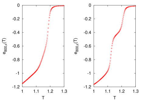
Figure 1: The energy density $e_{N,\epsilon}(T)$ for two particular sequences with $N=800$, one of which displays a two-step behaviour. Note the plateau at $e_{N,\epsilon}(T)=0$ in the coiled phase. The plotted region is the one around $T_{c}$ in which the energy varies more rapidly and there are evident differences in the behaviour from sample to sample. At lower temperatures quantities are nearly sample-independent and the energy density slowly decreases towards the fully double-stranded limit ${\overline{e_{min,\epsilon}}}=-1.5.$

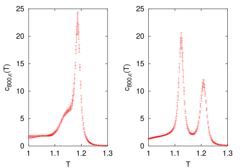
Figure 2: The specific heat $c_{N,\epsilon}(T)$ for two different disordered sequences with $N=800$ (the same sequences as in previous figure). Also in this case there is qualitative agreement with the experimentally observed behaviour in the differential melting curves, though the model should be improved in order of really comparing. For instance, particularly for short sequences, the plateau one gets in the coiled phase is usually higher than the low temperature one because of residual stacking energies which is an effect completely neglected here.

In Fig. 3 we plot our data on the disorder averaged specific heat for the considered chain lengths. This shows that, also in the presence of disorder, the maximum of the specific heat increases as a function of the chain length. Nevertheless, as discussed in detail in the following, it seems to behave as $N^{2\phi-1}$ with exponent smaller than one.

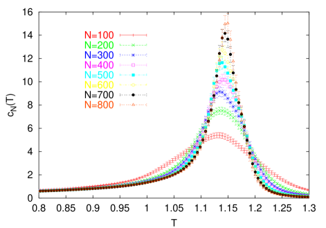
Figure 3: The disorder averaged specific heat for the considered chain lengths.

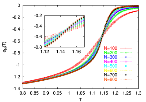
Figure 4: The disorder averaged energy density, for the considered chain lengths.

Then in Fig. 4 we present our data on the disorder averaged energy density. We note that curves corresponding to different $N$ values cross roughly at the same temperature $T_{c}\simeq 1.15$ within the errors (see the insert), therefore suggesting a transition still of first order. Actually this should mean a jump of the energy density in the thermodynamical limit, from zero for $T>T_{c}$ to the finite value $e(T_{c})\simeq-0.5$. Nevertheless, as displayed in Fig. 5a, the expected scaling law Eq. (5), which is well verified in the homogeneous case at least in the region $T\stackrel{{\scriptstyle\sim}}{{>}}T_{c}$, is here definitely not fulfilled with $\phi=1$. When fitting the data according to this scaling law (see Fig. 5b) one finds a slightly higher critical temperature value $T_{c}=1.155$ and a crossover exponent $\phi=0.8475$.

Since we were looking for a second order transition, i.e. for an exponent $\phi<1$, we required in the fit that data obey the scaling law on both sides of the critical temperature (for the random walk model in $3d$ [7], where the transition is of second order, a good scaling was observed on both sides of $T_{c}$). In any event we stress that by fitting data only in the high-temperature region $T\stackrel{{\scriptstyle\sim}}{{>}}T_{c}$ one would get a definitely lower value of the crossover exponent $\phi\sim 0.6$.

We note that the data roughly agree with the law but there are still corrections to scaling. We also checked that the disorder averaged number of contact density displays a similar behaviour (i.e. it follows the same scaling law).

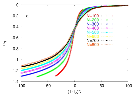
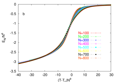
Figure 5: On the top we plot the disorder averaged energy density for the considered chain lengths as a function of $N(T-T_{c})$ with $T_{c}=1.15$. On the bottom we present the scaling law with $\phi=0.8475$ and $T_{c}=1.155$.

In Fig. 6 we present our data on the specific heat maximum, that would agree well with an exponent $\phi\simeq 0.85$ (our fit to the expected behaviour Eq. (6) gives $\phi=0.815$). However the data would also be compatible (within the errors) with $\phi=1$, if we were to neglect the smallest chain length $N=100$.

We tried, following [33], to analyze the data on the energy densities and the specific heats in terms of a reduced sample dependent temperature $T-T^{i}_{c}(N)$, where $T^{i}_{c}(N)$ is defined as the temperature for which the specific heat for sample $i$ and chain length $N$ reaches its maximum. This analysis leads to the same conclusion as the conventional one, that the disorder averaged energy density does not scale with a $\phi=1$ crossover exponent and the disorder averaged specific heat maximum seems to diverge more slowly than linearly with $N$ when taking into account all the considered chain lengths. We computed the average distance between the sample dependent critical temperatures $dT_{c}(N)=\frac{1}{{\cal N}({\cal N}-1)}\sum_{i\neq j}|{T_{c}}^{i}(N)-{T_{c}}^{j}(N)|$ (${\cal N}=128$ being the number of samples) which seems to go to zero for increasing chain lengths more slowly than $1/N$, again suggesting a second order transition.

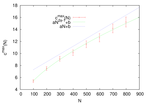
Figure 6: The behaviour of the specific heat maximum compared with a fit to the exponent $\phi=0.815$ and to $\phi=1$.

We looked at the probability distribution of the energy density at the critical temperature $T=1.15\simeq T_{c}$ (see Fig. 7a). In the homogeneous case it displays a large and flat scaling region extending to a value $e^{*}$ which do not depend on $N$, with deviations from the scaling law Eq. (7) for $e<e^{*}$ [7]. Here we find that the scaling law with $\phi=1$ is not well fulfilled. For the sake of comparison we also plot (in Fig. 7b) the behaviour of our data at the slightly higher temperature value $T=1.155$ with a crossover exponent $\phi=0.8475$.

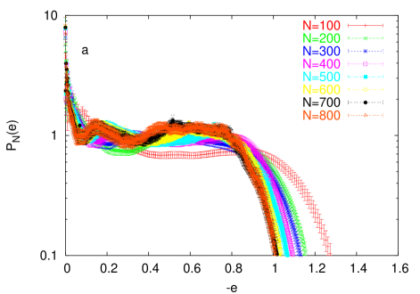
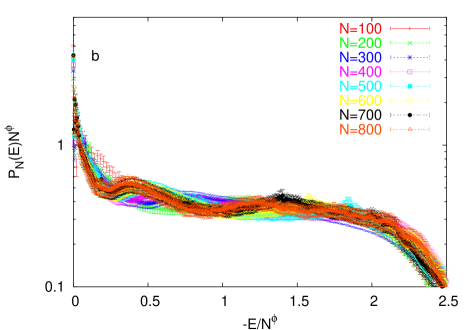
Figure 7: On the top we plot the disorder averaged probability distribution of the energy density at $T=1.15\simeq T_{c}$, $P_{N}(e)$ as a function of $-e$, which corresponds to the particular case of the corresponding scaling law with $\phi=1$, since $P_{N}(e)=N\>P_{N}(E/N)$. On the bottom we present the scaling law, $P_{N}(E)N^{\phi}$ as a function of $-E/N^{\phi}$, at $T_{c}=1.155$ with $\phi=0.8475$.

Let us now consider data on the disorder averaged probability distribution of the loop lengths ${P_{N}(l)}$ which are plotted in Fig. 8 at $T=1.15\simeq T_{c}$. We checked that the behaviour is very similar when temperature slightly varies. Again, a fit to the expected power law $\propto 1/l^{c}$ of the whole data set suggests an exponent $c<2$, i.e. a second order transition. Nevertheless, a closer inspection of the behaviour makes evident some curvature and when restricting the fit to the $l$ range $1<<l<<N$ (which is also the region in that the hypothesis $P_{N}(l)\propto 1/l^{c}$ should be better verified) we find larger $c$ values and the data for $N=100$ alone are definitely consistent with a first order transition.

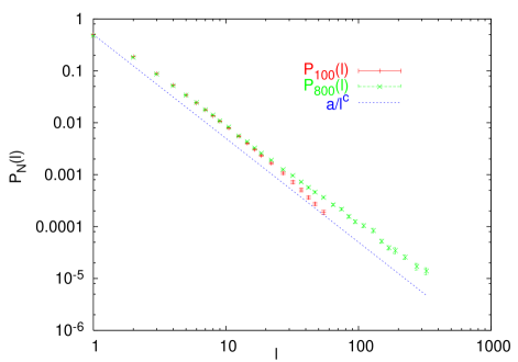
Figure 8: The disorder averaged probability distribution of the loop lengths at $T=1.15\simeq T_{c}$ for $N=100$ and $N=800$, compared to the behaviour $a/l^{c}$ with $c=2$.

To perform a more quantitative analysis, in Fig. 9 we consider [34] the momenta ${\overline{<l^{p}>}}$, which are expected to behave as $N^{\sigma_{p}}$. In particular the combination $\ln{\overline{<l^{p}>}}/\ln N$ is expected to be linear in $p$ on a large range of $p$ values and one should be able to evaluate $c-1$ by extrapolating the linear behaviour down to $p=0$. We effectively observe a quite linear behaviour for $p>1$ but by extrapolating we get the definitely different values $c=2.07$ for $N=100$ and $c=1.91$ for $N=800$. On the one hand data for the longest chain length should be the most meaningful, therefore confirming a second order transition; on the other hand it should be stressed that $P_{N,\epsilon}(l)$ is a difficult quantity to measure and we can not rule out the possibility that our statistics are inadequate for correctly evaluating it for the largest considered chain lengths.

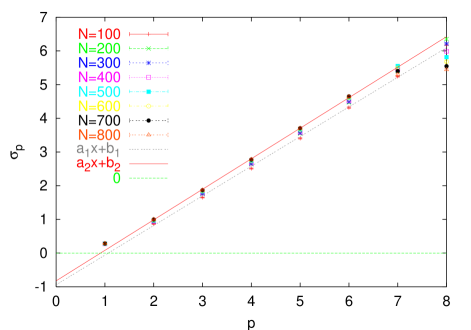
Figure 9: Data on $\sigma_{p}=\ln({\overline{<l^{p}>}})/\ln N$, from data on $P(l)$ at $T=1.15\simeq T_{c}$, plotted as function of $p$. The two fits give $c=2.07$ and $c=1.91$ respectively. We note that the linear behaviour is no more satisfied for $p>6$ in data corresponding to the largest $N$ values.

Nevertheless, the observed curvature on the $\log P_{N}(l,T_{c})\>vs\log(l)$ behaviour and the corresponding strong $N$-dependence in the obtained estimations could be related to finite size effects. One should note in particular that in the case of a second order transition the finite size corrections to the critical temperature (i.e. $T_{c}(N)-T_{c}(\infty)$) are expected to approach zero in the thermodynamical limit more slowly than $1/N$. Therefore, it could be misleading to fit the data according to the power law $P(l)\propto 1/l^{c}$ which is expected to be fulfilled only exactly at $T_{c}$. Moreover we have a large uncertainty on the evaluation of $T_{c}$ itself. For these reasons, in order to gain further insight into the behaviour of the system, we also attempt to compare the measures at the different temperatures considered with the more general law $P_{N}(l,T)\propto\exp(-l/\xi_{N}(T))/l^{c}$. This should allow to take partially into account finite size effects, by introducing a possible finite correlations length $\xi_{N}(T)$ which measures both the distance from the effective $T_{c}(N)$ and the finite size corrections to the thermodynamical limit correlation length.

Interestingly enough, in the temperature region $T\stackrel{{\scriptstyle\sim}}{{>}}T_{c}\sim 1.15$ one gets $1/\xi_{N}(T)$ compatible with zero within the errors (it can be also negative, though small) apart from the shortest chain lengths. In particular, data for $N=100$ are consistent with a detectably finite correlation length for all the temperatures studied. The corresponding evaluation of the exponent $c$ is in this case smaller than that found when the effect of the finite correlation length is neglected, giving usually $c<2$.

In detail, we performed three-parameter fits of data on $P_{N}(l,T)$ at different temperatures by neglecting both the very first and the last $l$ values. In particular the dependence on the number of neglected initial points has been studied by restricting the range to $l>5$ and to $l>2$. Whenever the fit gives a $1/\xi_{N}(T)<0$ unphysical value, the corresponding $c$ is estimated from the power law behaviour, i.e. by imposing $1/\xi_{N}(T)=0$. Moreover we also considered the fits to the power law in all the cases in which an inverse correlation length compatible with zero turns out, again by looking only at the $l>5$ range or at the whole $l>2$ one. Finally, we performed linear extrapolations to the $1/N\rightarrow 0$ limit.

Despite the introduction of the correlation length, the evaluations of $c$ seem generally to depend on temperature and on the number of initial points included in the fit, and its extrapolations turn out to be compatible with a first order transition. Nevertheless, the values obtained in the region $T\simeq T_{c}$, where the largest sizes can be fitted to the power law and which are therefore expected to be the most significant results, would definitively suggest a second order transition, characterized by a quite large crossover exponent $\phi\sim 0.9$. It should be noted that in this region one gets well compatible estimations from the different methods we used. In conclusion, the analysis is consistent with the initial qualitative observation on the $P(l)$ behaviour at $T\simeq T_{c}$, that the transition seems to be of second order when considering the longest chain lengths most meaningful.

It would be interesting to perform on $P_{N}(l,T)$ an analysis by introducing rescaled temperature but we unfortunately are not able to re-weigh data at different $T$ values in this case. To study whether this would not affect the qualitative behaviour, thereby confirming a second order transition, is left for future investigation.

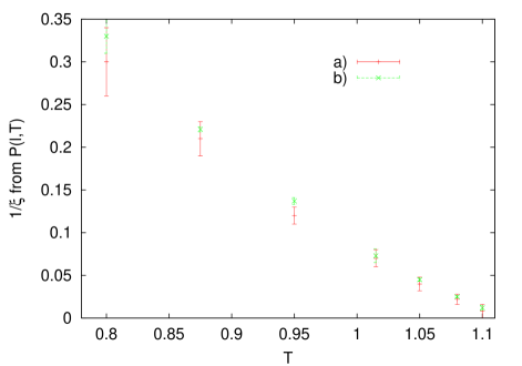
Figure 10: The results on the inverse correlation length $1/\xi(T)$ behaviour of the fits of data on $P_{N}(l,T)$ as obtained by different methods: a) For each $N$ and temperature the values are obtained from a three-parameter fit to the law $\propto\exp({-l/\xi_{N}(T))/l^{c}}$ neglecting only the very first (in particular the first two) and the last $l$ values. b) The same as in a) but restricting the considered range to $l>5$. In both cases values for different $N$ are linearly extrapolated to $1/N\rightarrow 0$ in order to give the plotted estimations. We stress that because of the fits involved the given errors are to be considered only very indicative, our uncertainty on the estimations being better expressed by the fluctuations between values obtained with the different methods.

Finally, we present in Fig. 10 data on the inverse correlation length, $1/\xi(T)$ as evaluated by extrapolating linearly to the limit $1/N\rightarrow 0$ values for the different chain lengths (here we only consider the temperature range where it is definitely larger than zero). The obtained qualitative behaviour suggests again a second order transition, since $1/\xi(T)$ seems to go to zero more rapidly than $(T_{c}-T)$. A fit to the expected power law behaviour $1/\xi(T)\propto(T_{c}-T)^{1/(c-1)}$ would give $c\sim 1.7$. We checked (on the $N=800$ data) that the qualitative behaviour of $\xi(T)$ does not change if we were to fit the data on $P_{N}(l,T)$ in the low temperature region according to the law (9) by imposing $c=2$ (or $c=2.1$).

As a last remark, we stress that our statistics are unfortunately inadequate for performing a more quantitative analysis, particularly on $\xi(T)$. Actually, because of the algorithm we are using, data on $P(l,T)$ in the low temperature range are reliable up to smaller $l$ values rather than in the region $T\stackrel{{\scriptstyle\sim}}{{>}}T_{c}$ (i.e. very long bubbles are usually not well sampled at low temperatures due to their negligible probability). Once again, we are led to the conclusion that the most significant results on $P(l,T)$ should be those obtained in the $T\simeq T_{c}$ region for the largest chain lengths, which is our best numerical evidence for the transition being of second order.

We have some preliminary numerical results on our model with different values of ${\cal R}$, where the crossing of the energy densities becomes less evident the more different the energies ${\epsilon_{AT}}$ and ${\epsilon_{GC}}$ are. The transition seems to be characterized by a varying crossover exponent which becomes smaller as ${\cal R}$ diminishes. In particular, by applying the scaling law to the disorder averaged energy densities we get $\phi\sim 0.8$ from data for ${\epsilon_{AT}}=1$ and ${\epsilon_{GC}}=4$, and $\phi\sim 0.7$ from data for ${\epsilon_{AT}}=0$ and ${\epsilon_{GC}}=1$. The $P(l)$ behaviour at the critical temperature would suggest similar values too, though also in these cases one gets different results by restricting the range to the region $1<<l<<N$. Here we only would like to mention that an alternative explanation for these results is that one is always looking at a first order transition but that the scaling laws of the homogeneous case are not well fulfilled anymore [33]. More extensive simulations would be necessary in order to clarify this issue.

5 Conclusions

Summarizing, we studied a disordered model for DNA denaturation transition consisting of two interacting self-avoiding chains in which we chose the two possible values of the interaction energy to be ${\epsilon}_{GC}=2{\epsilon}_{AT}$, distributed with equal probability. Despite of the extensive numerical simulations performed, it is difficult to definitively discriminate between a first order (as in the homogeneous case) and a smoother second order transition.

As a matter of fact, we find that the energy densities as a function of temperature for the different chain lengths considered roughly cross within the errors therefore suggesting a discontinuity of this quantity in the thermodynamical limit. However, the application of the scaling laws that are verified in the ordered case indicate a smoother second order transition with strong corrections to scaling.

When looking at the averaged probability distribution of the loop lengths, one gets again a crossover exponent $\phi$ definitely smaller than one from the data corresponding to the largest considered chain lengths. Nevertheless, data display some curvature also at $T\simeq T_{c}$ and higher values of the exponent are obtained when restricting the range to $1<<l<<N$. A momenta analysis of this probability distribution gives $c<2$ (i.e. $\phi<1$) only for the largest lengths. For a better understanding of this issue, we also attempted to perform a more general analysis on the whole considered temperature range by introducing a finite correlation length, with the aim of partially taking into account finite size effects. Results in the region $T\simeq T_{c}$ point towards a $c<2$ value and are our best numerical evidence of a second order transition. Anyway, it should be stressed that we get a quite large $c\sim 1.9$ and we can not rule out the possibility of a sharper (first order) transition.

During completion of this work, results appeared on the homogeneous Poland-Scheraga model [35] that seem to show how this model with the appropriate parameter values and the lattice SAW-DNA model are equivalent, even though the lattice model displays strong finite size corrections to scaling. Therefore a different kind of analysis on the disordered Poland-Scheraga model could help in better understanding the situation. To this extent, the recent study by Garel and Monthus [36] points towards the direction of a first order transition also in the presence of disorder, though the usual scaling laws seem to be not fulfilled. On the other hand, a very recent theoretical work [37] predicts that disorder should be relevant in this kind of models and that one should find a second order (or smoother) transition. In a nutshell, the situation appears far from being clarified and these simple models for DNA denaturation transition seem to deserve a careful analysis from the statistical mechanics point of view.

Finally, it should be pointed out that even if the transition is smoother in the presence of disorder the obtained value $c\sim 1.9$ for the considered interaction energies is definitely higher than the value $c=1.76276$ [32] which one gets in the homogeneous case when self-avoidance between different loops and segments is neglected. In the hypothesis that $c$ depends on the energy values one would expect, in the more realistic case of ${\epsilon}_{GC}$ closer to ${\epsilon}_{AT}$, an higher value of $c$ possibly indistinguishable from the case of a first order transition with $c>2$. In this sense the model seems relevant for the experimentally observed DNA denaturation, and which value of $c$ one should use in predictions based on Poland-Scheraga models as realistic as possible seems to be an open question.

References

- [1] R.M. Wartell and A.S. Benight, Phys. Rep. 126, 67 (1985).
- [2] D. Poland and H.A. Scheraga, J. Chem. Phys. 45, 1456 (1966); 45, 1464 (1966). For a review see D. Poland and H.A. Scheraga (eds.), Theory of Helix-Coil Transitions in Biopolymers, (Academic, New York, 1970).
- [3] M. Peyrard and A.R. Bishop, Phys. Rev. Lett. 62, 2755 (1989); T. Dauxois, M. Peyrard and A.R. Bishop Phys Rev. E 47, 684 (1993). S. Ares , Phys. Rev. Lett. 94, 035504 (2005).
- [4] S. Cocco and R. Monasson, Phys. Rev. Lett. 83, 5178 (1999).
- [5] V. Ivanov, Y. Zeng and G. Zocchi, Phys. Rev. E 70, 051907 (2004); V. Ivanov, D. Piontkovski and G. Zocchi, Phys. Rev. E 71, 041909 (2005).
- [6] N. Theodorakopoulos, T. Dauxois and M. Peyrard, Phys. Rev. Lett. 85, 6 (2000).
- [7] M.S. Causo, B. Coluzzi, and P. Grassberger, Phys. Rev. E 62, 3958 (2000).
- [8] Y. Kafri, D. Mukamel, and L. Peliti, Phys. Rev. Lett. 85, 4988 (2000).
- [9] E. Carlon, E. Orlandini, and A.L. Stella, Phys. Rev. Lett. 88, 198101 (2002).
- [10] T. Garel, C. Monthus, and H. Orland, Europhys. Lett. 55, 132 (2001); S.M. Bhattacharjee, Europhys. Lett. 57, 772 (2002); T. Garel, C. Monthus, and H. Orland, Europhys. Lett. 57, 774 (2002).
- [11] For a recent review in which the effects of self-avoidance in Poland-Scheraga models are critically discussed see C. Richard and A. J. Guttman, J. Stat. Phys. 115, 943 (2004).
- [12] R. D. Blake et al, Bioinformatics, 15, 370 (1999).
- [13] M.E. Fisher, J. Chem. Phys. 45, 1469 (1966).
- [14] Y. Kafri, D. Mukamel, and L. Peliti, Eur. Phys. J. B 27, 135 (2002).
- [15] B. Duplantier, Phys. Rev. Lett. 57, 941 (1986); J. Stat. Phys. 54, 581 (1989).
- [16] M. Baiesi, E. Carlon, E. Orlandini, and A. L. Stella, Eur. Phys. J. B 29, 129 (2002).
- [17] M. Baiesi, E. Carlon, and A. L. Stella, Phys. Rev. E 66, 021804 (2002);
- [18] M. Baiesi, E. Carlon, Y. Kafri, D. Mukamel, E. Orlandini, and A. L. Stella, Phys. Rev. E 67, 021911 (2003).
- [19] E. Orlandini, S. M. Bhattacharjee, D. Marenduzzo, A. Maritan, and F. Seno, J. Phys. A 34, L751 (2001).
- [20] R. Blossey and E. Carlon, Phys. Rev. E 68, 061911 (2003).
- [21] A. Hanke and R. Metzler, Phys. Rev. Lett. 90, 159801 (2003); Y. Kafri, D. Mukamel, and L. Peliti, Phys. Rev. Lett. 90 159802 (2003).
- [22] T. Garel and H. Orland, Biopolymers 75, 453 (2004).
- [23] D. Cule and T. Hwa, Phys. Rev. Lett. 79, 2375 (1997).
- [24] D.K. Lubensky and D.R. Nelson, Phys. Rev. Lett. 85, 1572 (2000); Phys. Rev. E 65, 031917 (2002).
- [25] A. B. Harris, J. Phys. C 7, 1671 (1974).
- [26] M. Aizenman and J. Wehr, Phys. Rev. Lett. 62, 2503 (1989); Phys. Rev. Lett. 64, 1311(E) (1990).
- [27] A. N. Berker, Physica A194, 72 (1993).
- [28] E. Eisenriegler, K. Kremer, and K. Binder, J. Chem. Phys. 77, 6296 (1982).
- [29] P. Grassberger, Phys. Rev. E 56, 3682 (1997).
- [30] H. Frauenkron, M.S. Causo, and P. Grassberger, Phys. Rev. E 59, R16 (1999).
- [31] S. Caracciolo, M.S. Causo, P. Grassberger, and A. Pelissetto, J. Phys. A 32, 2931 (1999).
- [32] P. Belohorec and B. Nickel, Accurate Universal and Two-parameter Model Results from a Monte-Carlo Renormalization Group Study, Preprint - University of Guelph (1997).
- [33] S. Wiseman and E. Domany, Phys. Rev. E 52, 3469 (1995); Phys. Rev. Lett. 81, 22 (1998); Phys. Rev. E 58, 2938 (1998).
- [34] C. Tebaldi, M. De Menech, and A.L. Stella, Phys. Rev. Lett. 83, 3952 (1999).
- [35] L. Schäfer, Can Finite Size Effects in the Poland-Scheraga Model Explain Simulations of a Simple Model for DNA Denaturation?, cond-mat/0502668
- [36] T. Garel and C. Monthus, J. Stat. Mech. P06004 (2005).
- [37] G. Giacomin and F.L. Toninelli, Smoothening effect of quenched disorder on polymer depinning transition, math.PR/0506431.