Origins of low- and high-pressure discontinuities of $T_{c}$ in niobium

Abstract

The discontinuities of $T_{c}$ in Niobium under pressure are examined by means of the pseudopotential plane-wave implementation of the electron-phonon coupling calculated from density-functional perturbation theory. Both low- and high-pressure discontinuities of $T_{c}$ have their origin in the Kohn anomalies and are caused by the low-frequency phonons, but the mechanism leading to the discontinuities is different in the two cases. The low-pressure anomaly is associated with a global decrease of the nesting factor in the whole Brillouin Zone and not to a visible change in the band structure. The high-pressure anomaly is instead connected with a well-pronounced change in the band structure.

I Introduction

Niobium is a superconductor with a quite high critical temperature, $T_{c}$= 9.25 K, for a simple metal. The experiments under pressure by Struzhkin et al. Struzhkin show discontinuities of $T_{c}$ at about 5 GPa and at 50-60 GPa. The low-pressure discontinuity manifests itself as an increase of $T_{c}$ by about 1 K. The high-pressure anomaly is associated with a decrease of the critical temperature. To date, the nature of these pressure-induced discontinuities is not clear. Previous theoretical studiesOstanin ; Ma ; Anderson-1 ; Anderson-2 agree in attributing the high-pressure anomalies to some visible change in the band structure. The low-pressure discontinuity of $T_{c}$, however, remains mysterious. The goal of this work is to give more information about the nature and the origin of the anomalous behavior of $T_{c}$ in niobium under pressure. In particular, we want to understand the role of Kohn anomaliesanomalies of the phonon spectra. Kohn anomalies are known to drastically change the critical temperature in superconductors and are believed to play a role in all body-centered cubic (bcc) metals Nb, Mo, V, Ta.anomalies-exp

Therefore, we look to the details of the electronic structure and dynamical properties of Nb at eight pressures in the range from -16 GPa to 78 GPa. We show that Kohn anomalies are responsible for both discontinuities, but the origin of the low-pressure Kohn anomaly is different from that of the high-pressure one. Both can be identified by a closer study of the Fermi-surface nesting and of the band structure.

The accurate calculation of the electron-phonon coupling $\lambda$ and of the spectral function $\alpha^{2}F$ is crucial for our problem. To this end we use density-functional perturbation theoryDFPT ; Review (DFPT) in a pseudopotential plane-wave approach. The Eliashberg function and the nesting factor require an integration of the double delta over the Fermi surface, which needs to be done with a high numerical accuracy. We give a few advices for an efficient calculation of the electron-phonon coupling. Some of the technical details, however, can be used in general for calculations of other properties which require an accurate numerical integration with the delta function.

This paper is organized as follows: In the next Section we remind the physical definitions and give some details of the calculation of electron-phonon interaction coefficients using Vanderbilt’s ultrasoft pseudopotentials.Vanderbilt In Sec. III, we give the technical details (Subsec. A) and present results for several properties under pressure: the lattice constant and bulk modulus (Subsec. B), the band structure and Fermi surface (Subsec. C), the phonon frequencies and linewidths (Subsec. D), and the Eliashberg function and electron-phonon coupling constant (Subsec. E). In Sec. IV, we discuss the origin of the anomalies, and we summarize in Sec. V. In the Appendix, we give numerical details for the calculation of the Eliashberg function.

II Electron-phonon coupling

II.1 Definitions

The Hamiltonian for the electron-phonon interaction is given in second quantization by

$$H_{el-ph}=\sum_{{\bf k}{\bf q}\nu}g_{{\bf k}+{\bf q},{\bf k}}^{{\bf q}\nu,mn}\;c_{{\bf k}+{\bf q}}^{\dagger m}c_{{\bf k}}^{n}\;(b_{-{\bf q}\nu}^{\dagger}+b_{{\bf q}\nu})$$ (1)

where $c_{{\bf k}+{\bf q}}^{\dagger m}$ and $c_{{\bf k}}^{n}$ are the creation and the annihilation operators for the quasiparticles with energies $\varepsilon_{{\bf k}+{\bf q},m}$ and $\varepsilon_{{\bf k},n}$ in bands $m$ and $n$ with wavevectors ${\bf k}+{\bf q}$ and ${\bf k}$, respectively; $b_{{\bf q}\nu}^{\dagger}$ and $b_{{\bf q}\nu}$ are the creation and the annihilation operators for phonons with energy $\omega_{{\bf q}\nu}$ and wavevector ${\bf q}$; the matrix element $g_{{\bf k}+{\bf q},{\bf k}}^{{\bf q}\nu,mn}$ describes the electron-phonon coupling. The coupling constants $g_{{\bf k}+{\bf q},{\bf k}}^{{\bf q}\nu,mn}$ define the spectral function, $\alpha^{2}F(\omega)$, its first reciprocal momentum, $\lambda$, and the superconducting electron-phonon coupling constant, $\lambda_{{\bf q}\nu}$, by the following set of equations:

$$\alpha^{2}F(\omega) = \frac{1}{N(\varepsilon_{F})}\sum_{mn}\sum_{{\bf q}\nu}\delta(\omega-\omega_{{\bf q}\nu})\sum_{\bf k}|g_{{\bf k}+{\bf q},{\bf k}}^{{\bf q}\nu,mn}|^{2}$$ (2)

$$\times\delta(\varepsilon_{{\bf k}+{\bf q},m}-\varepsilon_{F})\delta(\varepsilon_{{\bf k},n}-\varepsilon_{F}),$$

$$\lambda = 2\int\frac{\alpha^{2}F(\omega)}{\omega}d\omega=\sum_{{\bf q}\nu}\lambda_{{\bf q}\nu},$$ (3)

$$\lambda_{{\bf q}\nu} = \frac{2}{N(\varepsilon_{F})\omega_{{\bf q}\nu}}\sum_{mn}\sum_{\bf k}|g_{{\bf k}+{\bf q},{\bf k}}^{{\bf q}\nu,mn}|^{2}$$ (4)

$$\times\delta(\varepsilon_{{\bf k}+{\bf q},m}-\varepsilon_{F})\delta(\varepsilon_{{\bf k},n}-\varepsilon_{F}).$$

The quantity $N(\varepsilon_{F})$ is the density of states at the Fermi energy, $\varepsilon_{F}$, per both spins.

We introduce, after Allen,AllenGamma the phonon linewidth $\gamma_{{\bf q}\nu}$:

$$\gamma_{{\bf q}\nu} = 2\pi\omega_{{\bf q}\nu}\sum_{mn}\sum_{{\bf k}}|g_{{\bf k}+{\bf q},{\bf k}}^{{\bf q}\nu,mn}|^{2}\;$$ (5)

$$\times\delta(\varepsilon_{{\bf k}+{\bf q},m}-\varepsilon_{F})\delta(\varepsilon_{{\bf k},n}-\varepsilon_{F})$$

which enters the Eliashberg function, $\alpha^{2}F$, and the electron-phonon coupling constant, $\lambda_{{\bf q}\nu}$, as follows:

$$\alpha^{2}F(\omega) = \frac{1}{2\pi\;N(\varepsilon_{F})}\sum_{{\bf q}\nu}\frac{\gamma_{{\bf q}\nu}}{\omega_{{\bf q}\nu}}\delta(\omega-\omega_{{\bf q}\nu}),$$ (6)

$$\lambda_{{\bf q}\nu} = \frac{\gamma_{{\bf q}\nu}}{\pi\;N(\varepsilon_{F})\;\omega_{{\bf q}\nu}^{2}}.$$ (7)

II.2 Matrix elements of the electron-phonon interactions

Within DFPTDFPT ; Review the electron-phonon matrix elements can be obtained from the first-order derivative of the self-consistent Kohn-ShamDFT (KS) potential, $V_{KS}$, with respect to atomic displacements, $\vec{u}_{s{\bf R}}$ for the $s-$th atom in lattice position ${\bf R}$, as:

$$g_{{\bf k}+{\bf q},{\bf k}}^{{\bf q}\nu,mn}=\left(\frac{\hbar}{2\omega_{{\bf q}\nu}}\right)^{1/2}\langle\psi_{{\bf k}+{\bf q},m}|\Delta V_{KS}^{{\bf q}\nu}|\psi_{{\bf k},n}\rangle,$$ (8)

where $\psi_{{\bf k},n}$ is the $n-$th valence KS orbital of wavevector ${\bf k}$ and

$$\Delta V_{KS}^{{\bf q}\nu}=\sum_{\bf R}\sum_{s}\frac{\partial V_{KS}}{\partial\vec{u}_{s{\bf R}}}\cdot\vec{u}_{s}^{{\bf q}\nu}\frac{e^{i{\bf qR}}}{\sqrt{N}}$$ (9)

is the self-consistent first order variation of the KS potential, $N$ is the number of cells in the crystal, and $\vec{u}_{s}^{{\bf q}\nu}$ is the displacement pattern for phonon mode $\vec{v}_{s}^{{\bf q}\nu}$:

$$\vec{u}_{s}^{{\bf q}\nu}=\frac{\vec{v}_{s}^{{\bf q}\nu}}{\sqrt{M_{s}}}$$ (10)

The latter is obtained from the diagonalization of the dynamical matrix, $\varPhi^{\alpha\beta}_{ss^{\prime}}({\bf q})$:

$$\sum_{s^{\prime}\beta}\frac{\varPhi^{\alpha\beta}_{ss^{\prime}}({\bf q})}{\sqrt{M_{s}M_{s^{\prime}}}}v_{s^{\prime}\beta}^{{\bf q}\nu}=\omega_{{\bf q}\nu}^{2}v_{s\alpha}^{{\bf q}\nu}.$$ (11)

$M_{s}$ is the mass of atom $s$, $\alpha,\beta$ denote cartesian coordinates.

II.3 Matrix elements with ultrasoft pseudopotentials

The use of ultrasoft (US) pseudopotentials (PPs)Vanderbilt allows in many cases a significant reduction of the needed plane-wave kinetic energy cutoff, as compared with standard norm-conserving pseudopotentials. HBS1 ; KB ; MT This enables a more efficient calculation, at the price of introducing additional terms originating from the augmentation charges employed in this scheme.Vanderbilt A detailed description of DFPT with US PPs has been given elsewhere by Dal Corso.AndreaUS Here, we only briefly describe terms appearing in the electron-phonon coupling.

With US PPs the KS orbitals, $\psi_{{\bf k},n}$, satisfy a generalized eigenvalue problem

$$\left(-\frac{\nabla^{2}}{2}+V_{KS}-\varepsilon_{{\bf k},n}S\right)\psi_{{\bf k},n}=0$$ (12)

where the overlap matrix, S, is given by

$$S({\bf r}_{1},{\bf r}_{2}) = \delta({\bf r}_{1}-{\bf r}_{2})+\sum_{snm}q_{nm}$$ (13)

$$\times\beta_{n}({\bf r}_{1}-{\bf R}_{s})\beta_{m}^{\ast}({\bf r}_{2}-{\bf R}_{s}).$$

The charge correction $q_{nm}$, in the above formula, is defined with the augmentation functions, $Q_{nm}({\bf r}-{\bf R}_{s})$, as follows

$$q_{nm}=\int d^{3}r\;Q_{nm}({\bf r}-{\bf R}_{s}),$$ (14)

and the projector functions $\beta_{n}({\bf r}-{\bf R}_{s})$ are specific for the type of atom at the position ${\bf R}_{s}$, and are obtained from the atomic calculations.

The valence charge density is then computed as

$$\rho({\bf r}) = \sum_{{\bf k},i}(|\psi_{i}({\bf r})|^{2}+\sum_{smn}Q_{mn}({\bf r}-{\bf R}_{s})\langle\psi_{{\bf k},i}|\beta_{m}\rangle\langle\beta_{n}|\psi_{{\bf k},i}\rangle)$$ (15)

$$= \sum_{{\bf k},i}\int\int d^{3}r_{1}d^{3}r_{2}\psi_{{\bf k},i}^{\ast}({\bf r}_{1})K({\bf r};{\bf r}_{1},{\bf r}_{2})\psi_{{\bf k},i}({\bf r}_{2}),$$

where the sum over ${\bf k}$ and $i$ runs on occupied KS orbitals, the kernel

$$K({\bf r};{\bf r}_{1},{\bf r}_{2}) = \delta({\bf r}-{\bf r}_{1})\delta({\bf r}-{\bf r}_{2})+\sum_{snm}Q_{nm}({\bf r}-{\bf R}_{s})$$ (16)

$$\times\beta_{n}({\bf r}_{1}-{\bf R}_{s})\beta_{m}^{\ast}({\bf r}_{2}-{\bf R}_{s})$$

has been introduced for later convenience.

The KS selfconsistent potential in the US-PP scheme reads

$$V_{KS}({\bf r}_{1},{\bf r}_{2}) = V_{NL}({\bf r}_{1},{\bf r}_{2})$$ (17)

$$+\int d^{3}r\;V_{eff}({\bf r})\;K({\bf r};{\bf r}_{1},{\bf r}_{2}).$$

The effective potential, $V_{eff}$, contains the local, the Hartree and the exchange-correlation (xc) terms

$$V_{eff}({\bf r})=V_{loc}({\bf r})+\int d^{3}r_{1}\;\frac{\rho({\bf r}_{1})}{|{\bf r}_{1}-{\bf r}|}+V_{xc}({\bf r}),$$ (18)

while the nonlocal term generalizes the usual Kleinman-BylanderKB form allowing several projectors for a given angular momentum component

$$V_{NL}({\bf r}_{1},{\bf r}_{2})=\sum_{snm}D_{nm}^{0}\;\beta_{n}({\bf r}_{1}-{\bf R}_{s})\beta_{m}^{\ast}({\bf r}_{2}-{\bf R}_{s}).$$ (19)

When augmentation charges vanish ($Q_{nm}=0$) the above formulas reduce to the standard norm-conserving formulation.

In order to generalize Eq. (8) to the case of US PPs, one needs to compute first order perturbation theory in presence of overlap matrix, $S$, as below

$$g_{{\bf k}+{\bf q},{\bf k}}^{{\bf q}\nu,mn}=\langle\psi_{{\bf k}+{\bf q},m}|\Delta V_{KS}^{{\bf q}\nu}-\varepsilon_{{\bf k},n}\Delta S|\psi_{{\bf k},n}\rangle,$$ (20)

where

$$\Delta S=\sum_{\bf R}\sum_{s}\frac{\partial S}{\partial\vec{u}_{s{\bf R}}}\cdot\vec{u}_{s}^{{\bf q}\nu}\frac{e^{i{\bf qR}}}{\sqrt{N}},$$ (21)

and $\Delta V_{KS}^{{\bf q}\nu}$ is given by Eq. (9).

The derivative of the Kohn-Sham potential is given in Ref. [AndreaUS, ] and for gradient-corrected functionals in Ref. [GGA, ].

III Results for niobium under pressure

III.1 Technical details

The calculations of the ground-state electronic and vibrational properties of Nb were performed using the Local-Density Approximation (LDA) and an ultrasoft pseudopotential. A kinetic energy cut-off of 45 Ry (270 Ry) was chosen for the expansion into plane waves of the wavefunctions (density). Such high cut-offs were necessary to obtain accurate values for some ”strategic” low-frequency phonons, located mostly near the $\Gamma$-point. In fact, even small errors in this region of the spectrum lead to large relative errors in the estimate of the $\alpha^{2}F$ function and of $\lambda$.

The integration over the Brillouin zone (BZ) requires special techniques to account for the Fermi surface. We used the broadening technique proposed in Ref. [Paxton, ] with a smearing parameter of 0.03 Ry (which was testedSdG-broad to reproduce well the experimental spectra). The grids for the electronic BZ integration (k-grid) and for the phononic BZ integration (q-grid) have been chosen according to the Monkhorst-Pack scheme.mesh

Details of the numerical quadrature used to evaluate the double-delta term appearing in Eq.(2), together with convergence tests, are given in the Appendix.

All calculations were performed using the quantum-espressoespresso suite of codes.

III.2 Structural properties

Niobium in the body-centered cubic structure was studied at eight values of the lattice parameter from 6.34 a.u. to 5.64 a.u in steps of 0.1 a.u. These lattice parameters correspond to pressures ranging from -16.6 GPa to 78.4 GPa. The results are reported in TABLE 1. The calculated static equilibrium lattice constant (zero-point motion and thermal effects not included) is about 6.14 a.u., slightly underestimating (as it usually happens within LDA) the experimental valueAshcroft of 6.24 a.u. The calculated bulk modulus at the theoretical equilibrium lattice is 192 GPa, versus a room-temperature experimental valuebulkmod of 170 GPa and a calculated value of 162 GPa at the experimental lattice parameter of 6.24 a.u. The calculated bulk modulus is very sensitive to the volume: it varies by more than a factor three in the considered range of pressures.

$a$	V/V0	$P$	$B$
6.34	1.10	-16.6	134
6.24	1.05	-9.5	162
6.14	1.00	-0.6	192
6.04	0.95	10.0	220
5.94	0.91	22.9	249
5.84	0.86	38.8	308
5.74	0.82	56.7	354
5.64	0.78	78.4	424

Table 1: The lattice constant $a$ (in a.u.), the corresponding volume ratio V/V₀, the pressure $P$ (in GPa), and bulk modulus $B$ (in GPa) calculated for BCC niobium crystal at several pressures. The experimental lattice constantAshcroft is 6.24 a.u. and the bulk modulusbulkmod is 170 GPa.

III.3 Band structure and Fermi surface

The evolution of the band structure as a function of pressure is presented in FIG. 1, showing no qualitative change in the electronic states at the Fermi surface up to about 38.8 GPa. From 56.7 GPa to 78.4 GPa, we observe some changes along the $\Gamma$-H and $\Gamma$-N lines.

A 3D picture of the Fermi surface at ambient pressure and 56.7 GPa is drawn in FIG. 2. The lower energy band forms the octahedron centered at the $\Gamma$-point. With increasing pressure, this octahedron shrinks and it becomes surrounded by six little ellipsoids when the previously described band-structure changes on the $\Gamma$-H line appear. Around N-point, the Fermi surface forms ellipsoids that are disconnected at lower pressure and becomes connected by necks to the four neighboring ellipsoids above 56.7 GPa. In addition, a complicated open sheet structure, often referred as ”jungle gym”, extends from $\Gamma$ to the H points in the BZ.

Our results are in good agreement with the detailed studies of Anderson et al. Anderson-1 for the band structure and of Ref. [Anderson-2, ] for the Fermi surface.

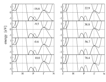
Figure 1: The band structures of niobium at several pressures (in GPa).

Figure 2: Fermi surfaces from two bands (the lower energy band in the left panels and the higher energy band in the right panels) at ambient pressure (top panels) and at 56.7 GPa (bottom panels). Pictures obtained with the XCrySDen package.xcrysden

III.4 Phonon frequencies and linewidths

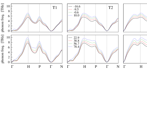
Figure 3: Phonon dispersions in niobium at several pressures (in GPa), for the two transverse modes (left and medium panels, notation ”T1” and ”T2”) and the longitudinal mode (right panels, notation ”L”); the scale on the vertical axis is the same for all three modes.

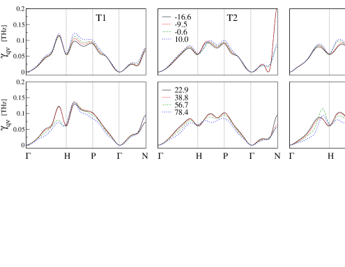
Figure 4: Phonon linewidths (in THz) in niobium at several pressures (in GPa). The three modes of $\gamma_{{\bf q}\nu}$ correspond to the three phonon modes shown in FIG. 3; the scale on the vertical axis is the same for all three modes.

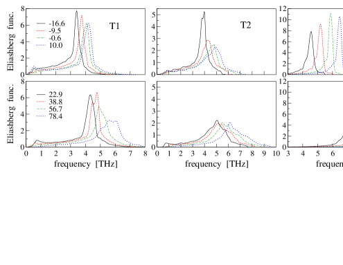
Figure 5: Eliashberg function, $\alpha^{2}F$, in niobium at several pressures (in GPa); the scale on the horizontal axis is the same, within a given mode, for all pressures.

The phonon spectra are presented in FIG. 3. We observe an overall increase in phonon frequencies with pressure, especially at H, P and N high-symmetry points. Close to the $\Gamma$-point along the $\Gamma$-H symmetry line, very low frequency phonon modes with an anomalous pressure dependence can be observed. At both the experimental and the calculated equilibrium lattice constants, the two transverse modes (T1 and T2 in the following) display a very flat dispersion close to $\Gamma$-point. At variance with all other modes in the BZ, the T1 and T2 modes along $\Gamma$-H line soften with pressure (between $\approx$10 to $\approx$55 GPa in our calculations). This anomalous, non-monotonic, dispersion relation eventually disappears and become a smooth curve at the highest pressure we have considered.

The phonon linewidths $\gamma_{{\bf q}\nu}$ have a weak dependence upon pressure (see FIG. 4), with two important exceptions: i) at low pressure, large variations in phonon linewidth occur for the T2 and L modes near the N high-symmetry point, and ii) at high pressure (above $\approx$55 GPa), a significant reduction in linewidth is observed in many parts of the BZ, especially along the $\Gamma$-H direction.

III.5 Eliashberg function and electron-phonon coupling constant

By integrating the calculated phonon linewidths and frequencies we can obtain Eliashberg $\alpha^{2}F(\omega)$ function, Eq. (6), that we present in FIG. 5 for the three phonon branches separately. As a general feature, all peaks in $\alpha^{2}F(\omega)$ move to higher frequency with pressure, as expected from the global positive frequency shift with pressure visible in FIG. 3. For the T1 and T2 modes the height of the main peak decreases with pressure, while for the L mode the maximal height of the peak appears at the equilibrium lattice constant.

Our calculated $\lambda$ and the density of states at the studied pressures are presented in TABLE 2. The pressure behavior of the electron-phonon coupling constant is similar to what could be expected from the experimental pressure dependence for $T_{c}$: $\lambda$ shows a positive jump at low pressure and decreases significantly at high pressure.

$P$		$N(\varepsilon_{F})$		$\lambda$		$\sim T_{c}^{exp}$
-16.6		11.41		1.91		-
-9.5		10.80		1.60		-
-0.6		10.12		1.41		9.2
10.0		9.69		1.65		10.0
22.9		9.16		1.47		9.8
38.8		8.55		1.29		9.7
56.7		7.71		1.10		9.5
78.4		6.55		0.86		8.8

Table 2: The parameters of niobium under pressure, $P$ (in GPa): the electronic density of states at the Fermi surface $N(\varepsilon_{F})$ (states per spin and per Ry), the electron-phonon coupling constant $\lambda$, and the experimental critical temperature $T_{c}^{exp}$ from Ref. [Struzhkin, ].

A good review of theoretical works on the electron-phonon coupling in Nb at ambient pressure is given by Solanki et al. in Ref. [Solanki, ], where the reported values of the electron-phonon coupling constant range from 0.59, obtainedAnderson-1 from augmented plane-wave method (APW), to 1.52, obtainedlambda-1.52 later from the same method. More recently, SavrasovSav-lambda obtained a value of 1.26, Bauer et al. Bauer obtained a value of 1.33, while our results for $\lambda$ at ambient pressure is 1.41.

We notice that the main reason for the spread in the reported values of $\lambda$ is the difference in calculated values for $N(\varepsilon_{F})$, entering the definition of $\lambda$ in the denominator (Eqs. (2)-(4)). In fact a large value of 14.1 (states per spin and per Ry) for the DOS and a small value of 0.59 for $\lambda$ have been reported in Ref. [Anderson-1, ], while a value of 8.89 for the DOS and $\lambda$=1.52 have been reported in Ref. [lambda-1.52, ]. Consistent with this trend, our calculated DOS of 10.12 at ambient pressure is somewhat lower than the DOS of 10.21 obtained by Savrasov,Sav-lambda , while other authors obtained $\sim 11$ (Ref. [Ostanin, ]), 11.77 (Ref. [Singalas, ]), and 9.84 (Ref. [Crabtree, ]).

The experimental values of $\lambda$ obtained from the electronic tunneling spectroscopylambda-exp1 ; lambda-exp2 are 1.04 and 1.22, while Haas-van Alphen dataCrabtree yield $\lambda=1.33$.

IV Discussion

After examination of the phonons and the electron-phonon coupling, we notice that the decrease of $\lambda$ at high pressure can be easily related to the decrease of the $\alpha^{2}F(\omega)$ peak and to its shift toward higher frequencies for all modes.

The origin of the increase of $\lambda$ at low pressure between $\approx$0 GPa and $\approx$10 GPa is instead more difficult to trace. We found out that it is mainly determined by the anomalous dispersion of the T1 and T2 modes close to $\Gamma$-point (see FIG. 3) in the frequency region below 1 THz, that determines a low-frequency peak in the Eliashberg function of the T1 mode above 10 GPa. This peak is instead absent at ambient pressure and reappears for an expanded lattice only at about -16 GPa.

It has been shown Vonsovsky for the Eliashberg model that the contribution to $T_{c}$ from acoustic modes close to the $\Gamma$-point vanishes. For the low-frequency modes which are associated to Kohn anomalies, however, we can expect important contribution to $T_{c}$ because phonon softening may occur with a finite phonon linewidth. Therefore, the region near $\Gamma$ can give a very large contribution to the electron-phonon coupling in niobium for all studied pressures (see TABLE 2).

Let us now consider the band structure. In order to explain low-pressure anomalies in $T_{c}$, Struzhkin et al.Struzhkin proposed the existence of necks between the ellipsoids around N and the ”jungle gym” open sheet extending from $\Gamma$ to H along the $\Gamma$-$\Sigma$ line at a pressure below 5 GPa, and the disappearance of these features at the higher pressures. Our calculations do not support this suggestion. The detailed analysis of the Fermi surface reported by Ostanin et al. Ostanin gives results close to ours. Previous theoretical Solanki ; Anderson-2 ; Neve ; lambda-1.52 ; fermi-1 ; fermi-2 and experimental Anderson-2 ; fermi-3 ; fermi-4 investigations of the Fermi surface also did not detect any changes at low pressure.

One can, therefore, connect the high-pressure decrease in electron-phonon coupling to changes in the band structure, while the origin of the low-pressure anomaly remains unclear. Therefore, we need a different tool in order to detect tiny features of the Fermi surface.

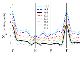
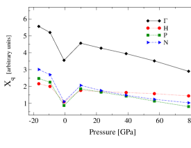
Figure 6: The nesting factor, $X_{\bf q}$, of the Fermi surface in niobium at eight studied pressures (in GPa), for selected high-symmetry lines (top panel) and high-symmetry points (bottom panel).

Figure 7: The isosurface of the nesting factor in the whole BZ, $X_{\bf q}=1.0$ (arbitrary units), for niobium at pressures of -0.6 GPa (left panel) and 10.0 GPa (right panel). Pictures obtained with the XCrySDen package.xcrysden

We propose to look closer at Fermi surface nesting by plotting the dispersion of the nesting factor:

$$X_{\bf q}=\sum_{\bf k}\delta(\varepsilon_{{\bf k}}-\varepsilon_{F})\delta(\varepsilon_{{\bf k}+{\bf q}}-\varepsilon_{F}).$$ (22)

Large nesting factors correspond to large regions of the Fermi surface being connected by the nesting vector, $\bf q$, and are expected to correspond to large electron-phonon couplings.

In FIG. 6, the factor $X_{\bf q}$ is reported as a function of pressure. This quantity has been computed numerically using the smearing technique with the broadening of 0.03 Ry. The maximal nesting takes place at the $\Gamma$-point with much smaller maxima at the high-symmetry points H, P and N, and in the middle of the lines: $\Gamma$-H, H-P, P-$\Gamma$ and $\Gamma$-N. The nesting factor decreases monotonically with increasing pressure in the whole BZ except around ambient pressure (0-10 GPa). At the equilibrium lattice constant, a large damping of the nesting factor moves the whole nesting curve below its value at 38.8 GPa and makes it even similar to the curve drawn for the pressure of 56.7 GPa.

The damping of the nesting factor close to ambient pressure occurs in the whole BZ, as we can see in FIG. 7 in comparison to nesting for a pressure of 10.0 GPa. This damping explains the jump in the total electron-phonon coupling constant which happens below and above the ambient pressure (see TABLE 2).

V Summary

We investigated the origin of the two discontinuities of the superconducting critical temperature, observed in Niobum at low pressure, about 5 GPa, and at high pressure, about 60 GPa. Struzhkin For this purpose, we developed computational tools for the accurate calculation of the electron-phonon coupling.

We find that the anomalous behavior of $T_{c}$ in Nb under pressure originates in Kohn anomalies close to the $\Gamma$-point in the BZ, so the measured discontinuities are caused by low-frequency phonons. In agreement with previous authors,Ostanin ; Ma ; Anderson-1 ; Anderson-2 we find that the high-pressure discontinuity of $T_{c}$ is associated to a visible change in the band structure. As for the low-pressure discontinuity, we notice that such anomaly shows up as a general decrease of the nesting factor without any visible change in the shape of the Fermi surface. Such a decrease is uniform in the whole BZ, explaining why previous calculations, Refs. [Ostanin, ; Ma, ], did not detect any anomaly in the electronic structure of Nb near ambient pressure. The total electron-phonon coupling constant varies with pressure as expected from the measured critical temperatures.

In conclusion, both discontinuities of $T_{c}$ in niobium, at low and high pressures, can be reproduced when the electron-phonon spectral function is calculated accurately, and the anomalies can be explained by the closer look into the details of the Fermi-surface nesting and the band structure.

Appendix A Implementation details and test calculations

The electron-phonon coupling constant $\lambda$ and the spectral function $\alpha^{2}F(\omega)$ are defined by a double-delta integration on the Fermi surface (Eqs. (2) and (4)). The accurate calculation of these integrands requires a very dense sampling in both the electronic (k) and the phononic (q) grids. One can use either the broadening technique broadening or the tetrahedron method.tetra We choose the former to perform the quadrature on the Fermi surface, and the latter to evaluate the electron-phonon and phonon densities of states as functions of the vibrational frequencies. In the broadening scheme, a finite energy width is attributed to each state. For any function $f$ which has to be integrated with the double-delta, one can use the formula

$$I = \int d{\bf k}\int d{\bf q}\;f({\bf k},{\bf q})\;\delta(\epsilon_{\bf k}-\epsilon_{F})\delta(\epsilon_{{\bf k}+{\bf q}}-\epsilon_{F})$$ (23)

$$\simeq {\Omega_{BZ}^{2}\over N_{k}N_{q}}\sum_{\bf k}\sum_{\bf q}f({\bf k},{\bf q})\;\frac{1}{\sqrt{2\pi}\sigma}exp\left(-\frac{(\epsilon_{\bf k}-\epsilon_{F})^{2}}{\sigma^{2}}\right)$$

$$\times\frac{1}{\sqrt{2\pi}\sigma}exp\left(-\frac{(\epsilon_{{\bf k}+{\bf q}}-\epsilon_{F})^{2}}{\sigma^{2}}\right),$$

where $\sigma$ is the broadening, $N_{k}$ and $N_{q}$ the number of k- and q-points, $\Omega_{BZ}$ the volume of the BZ. For infinitely dense grids of k- and q-points, convergence of the integrand is achieved when $\sigma$ approaches zero. For finite grids, however, one has to find a range of $\sigma$ values yielding close results for the integrands at different grids. In metals like Nb the presence of Kohn anomalies in the phonon spectra sets additional requirements for the accuracy. Thus, it is expected that the aforementioned integrands have to be calculated at very dense k-point and q-point grids.

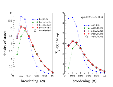
Figure 8: The density of states and the double-delta integrand on the Fermi surface of Nb.

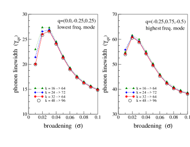
Figure 9: The phonon linewidth $\gamma_{{\bf q}\nu}$ for two selected q-vectors.

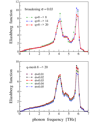
Figure 10: The Eliashberg function of Nb for fixed broadening $\sigma$=0.03 Ry and different q-grid (top panel) and the Eliashberg function for fixed q-grid and different broadening $\sigma$ (bottom panel).

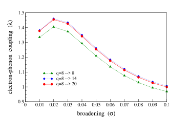
Figure 11: The total electron-phonon coupling $\lambda$ of Nb for different q-grids as a function of broadening $\sigma$.

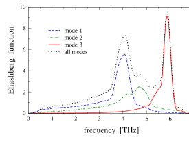
Figure 12: The Eliashberg function for Nb at calculated equilibrium lattice constant (6.14 a.u.).

Since the electron-phonon coupling matrix elements are smooth functions of k and q, we resort to an interpolation procedure. For a chosen k- and q-vector grid, we calculate matrix elements $g_{\bf k+q,k}^{{\bf q}s\alpha,mn}$, defined as in Eq. (8) but with respect to the displacement of a single atom $s$ along cartesian component $\alpha$. For each q-vector we make a linear interpolation in k-space of the matrix elements to a denser k-vector grid. We then perform the integration, using the denser grid and gaussian broadening as in Eq. (23), of auxiliary phonon linewidths $\widetilde{\gamma}^{\alpha\beta}_{ss^{\prime}}({\bf q})$, defined as:

$$\widetilde{\gamma}^{\alpha\beta}_{ss^{\prime}}({\bf q}) = \sum_{mn}\sum_{{\bf k}}(g_{{\bf k+q,k}}^{{\bf q}s\alpha,mn})^{*}g_{{\bf k+q,k}}^{{\bf q}s^{\prime}\beta,mn}\;$$ (24)

$$\times\delta(\varepsilon_{{\bf k}+{\bf q},m}-\varepsilon_{F})\delta(\varepsilon_{{\bf k},n}-\varepsilon_{F}).$$

These are related to the $\gamma_{{\bf q}\nu}$ of Eq. (5) through the relation

$$\gamma_{{\bf q}\nu}=2\pi\omega_{{\bf q}\nu}\sum_{s\alpha}\sum_{s^{\prime}\beta}(u^{{\bf q}\nu}_{s\alpha})^{*}\widetilde{\gamma}^{\alpha\beta}_{ss^{\prime}}({\bf q})u^{{\bf q}\nu}_{s^{\prime}\beta}.$$ (25)

Symmetry is exploited to reduce the number of k- and q-points used in the calculation. A convenient way to achieve such a goal is to perform symmetrization. Let us denote with $T^{\alpha\beta}$ the symmetry operators of the small group of q (i.e. the subgroup of crystal symmetry that leaves q unchanged). We restrict summation on k-points to the irreducible BZ calculated with respect to the small group of q. Then symmetrization is performed, separately for each q-vector, as follows:

$$\widetilde{\gamma}^{\alpha\beta}_{ss^{\prime}}({\bf q}) = \sum_{\alpha^{\prime}\beta^{\prime}}\;T^{\alpha\alpha^{\prime}}T^{\beta\beta^{\prime}}\widetilde{\gamma}^{\alpha^{\prime}\beta^{\prime}}_{T(s)T(s^{\prime})}({\bf q})$$ (26)

$$\times exp\left(i\vec{\bf q}\cdot(\vec{\tau}_{s}-\vec{\tau}_{T(s)}-\vec{\tau}_{s^{\prime}}+\vec{\tau}_{T(s^{\prime})})\right).$$

In the above formula, atom $s$ with atomic position $\vec{\tau}_{s}$ transform into atom $T(s)$ with atomic position $\vec{\tau}_{T(s)}$ after application of operation $T$. The symmetrized matrix at each q is subsequently rotated, using the remaining crystal symmetries that are not in the small group of q, and the symmetrized matrices at all q-vectors in the star of q are thus obtained with minimal computational effort. The same procedure can be applied to dynamical matrices, Eq. (11).

Once the electron-phonon coupling matrix of Eq. (24) are calculated on a q-vector grid, it is possible to perform Fourier interpolation and to interpolate to a finer grid. In this way, the integration in the q space needed to calculate $\alpha^{2}F(\omega)$, Eq. (2), and $\lambda$, Eq. (3), can be accurately performed with a reasonable computational effort.

Let us turn now to some numerical experiments. FIG. 8 shows the density of states for Nb (left panel) and the double-delta integrand of a constant function (right panel) at the Fermi surface for a selected q-vector, as a function of the broadening $\sigma$ and of the Monkhorst-Packmesh k-point grid. For large enough $\sigma$ the results for different grids – except the (8,8,8) grid which is too coarse – converge to the same values, which however depend on $\sigma$. For small enough $\sigma$ different grids yield different results. Since we are interested in the $\sigma\rightarrow 0$ limit, we have to choose a grid of an affordable size that yields converged results for a $\sigma$ as small as possible. A reasonable choice is the (64,64,64) grid with $\sigma$=0.02 Ry, yielding a DOS at the Fermi energy about 10.1 states per spin and per Ry. The convergence of the double-delta function is a little bit slower than that of a single-delta.

The phonon linewidths, $\gamma_{{\bf q}\nu}$, for two selected phonons q$\nu$ are displayed in FIG. 9. The self-consistent calculations were performed i) at the k-grids of (16,16,16) and (32,32,32), interpolated to a denser (64,64,64) grid; ii) at the (24,24,24) k-grid, interpolated to (72,72,72); iii) at the (48,48,48) k-grid, interpolated to (96,96,96). The integration weights for the k-space quadrature, i.e. the gaussians centered around the single-particle energies, were obtained from the accurate self-consistent calculation at the corresponding dense grids. As one can see in FIG. 9, the convergence in k-points is obtained quite easily even for the SCF calculation at the grid (16,16,16).

In order to obtain the spectral function $\alpha^{2}F(\omega)$ one needs to perform the q-space quadrature of the phonon linewidths; Eq. (6). For the phonon and the electron-phonon densities of states at given frequency $\omega$, we employ the tetrahedron method within the scheme proposed by Blöchl.Bloechl FIG. 10 (upper panel) shows the Eliashberg function, $\alpha^{2}F$, of Nb for q-grid (8,8,8), without interpolation and interpolated into denser grids. This has been done for a fixed broadening, $\sigma$=0.03 Ry. The lower panel of the same figure shows the $\alpha^{2}F$ function at the q-grid of (8,8,8) interpolated to (20,20,20)-point grid for several broadenings $\sigma$.

In FIG. 11, we report the variation of total electron-phonon coupling constant $\lambda$ with the broadening $\sigma$ for three q-meshes.

In FIG. 12, we present the electron-phonon density of states for niobium under ambient pressure. We fit the curve of the spectral function with cubic splines NR for a finer plot.

References

- (1) V. V. Struzhkin, Y. A. Timofeev, R. J. Hemley and H.-k. Mao, Phys. Rev. Lett. 79, 4262 (1997).
- (2) S. A. Ostanin, V. Yu. Trubitsin, S. Yu. Savrasov, M. Alouani and H. Dreyssé, Comp. Mat. Sc. 17, 202 (2000).
- (3) J. S. Tse, Z. Li, K. Uehara, Y. Ma and R. Ahuja, Phys. Rev. B 69, 132101 (2004).
- (4) J. R. Anderson, D. A. Papaconstantopoulos, J. W. McCaffrey and J. E. Shirber, Phys. Rev. B 7, 5115 (1973).
- (5) J. R. Anderson, D. A. Papaconstantopoulos and J. E. Shirber, Phys. Rev. B 24, 6790 (1981).
- (6) W. Kohn, Phys. Rev. Lett. 2, 393 (1959).
- (7) A. D. B. Woods and S. H. Chen, Solid State Commun. 2, 233 (1964);A. D. B. Woods, Phys. Rev. 136, A781 (1964); Y. Nakagawa and A. D. B. Woods, Phys. Rev. Lett. 11, 271 (1963); J. Peretti, I. Pelah and W. Kley, Phys. Lett. 3, 105 (1962).
- (8) S. Baroni, P. Giannozzi and A. Testa, Phys. Rev. Lett. 58, 1861 (1987).
- (9) S. Baroni, S. de Gironcoli, A. Dal Corso and P. Giannozzi, Rev. Mod. Phys. 73, 515 (2001).
- (10) D. Vanderbilt, Phys. Rev. B 41, R7892 (1990).
- (11) P. B. Allen, Phys. Rev. B 6, 2577 (1972).
- (12) P. Hohenberg and W. Kohn, Phys. Rev. 136, B864 (1964); W. Kohn and L. J. Sham, Phys. Rev. 140, A1133 (1965).
- (13) D. R. Hamann, M. Schlüter and C. Chiang, Phys. Rev. Lett. 43, 1494 (1979); G. B. Bachelet, D. R. Hamann and M. Schlüter, Phys. Rev. B 26, 4199 (1982).
- (14) L. Kleinman and D. M. Bylander, Phys. Rev. Lett. 48, 1425 (1982); D. L. Bylander and L. Kleinman, Phys. Rev. B 43, 12070 (1991).
- (15) N. Troullier and J. L. Martins, Phys. Rev. B 43, 1993 (1991).
- (16) A. Dal Corso, Phys. Rev. B 64, 235118 (2001); A. Dal Corso, A. Pasquarello, A. Baldereschi, Phys. Rev. B 56, 11372 (1997).
- (17) A. Dal Corso and S. de Gironcoli, Phys. Rev. B 62, 273 (2000).
- (18) M. Methfessel and A. T. Paxton, Phys. Rev. B 40, 3616 (1989).
- (19) S. de Gironcoli, Phys. Rev. B 51, 6773 (1995).
- (20) H. J. Monkhorst and J. D. Pack, Phys. Rev. B 13, 5188 (1976).
- (21) http://www.quantum-espresso.org
- (22) R. L. Barns, J. Appl. Phys. 39, 4044 (1968); Landolt-Börnstein, Numerical Data and Functional Relationships in Science and Technology, edited by O. Madelung, Group III: Crystal and Solid State Physics, vol. 14: Structure Data of Elements and Intermetallic Phases, (Springer Verlag, Berlin 1988).
- (23) A M. James and M. P. Lord, Macmillan’s Chemical and Physical Data, (Macmillan, London, UK, 1992).
- (24) A. Kokalj, Comp. Mater. Sci., 2003, Vol. 28, p. 155. Code available from http://www.xcrysden.org/.
- (25) A. K. Solanki, R. Ahuja and S. Auluck, Phys. Stat. Sol. B 162, 497 (1990).
- (26) L. L. Boyer, D. A. Papaconstantopoulos and B. M. Klein Phys. Rev. B 15, 3685 (1997).
- (27) S. Y. Savrasov and D. Y. Savrasov, Phys. Rev. B 54, 16487 (1996).
- (28) R. Bauer, A. Schmid, P. Pavone and D. Strauch, Phys. Rev B 57, 11276 (1998).
- (29) M. M. Singalas and D. A. Papaconstantopoulus, Phys. Rev. B 50, 7255 (1994).
- (30) G. W. Crabtree, D. H. Dye, D. P. Karim and D. D. Koelling, Phys. Rev. Lett. 42, 390 (1979).
- (31) E. L. Wolf, Principles of Electronic Tunneling Spectroscopy, (Oxford University Press, New York, 1985).
- (32) M. J. Bostock, M. L.A. Mac Vicar, G. B. Arnold, J. Zasadziński and E. L. Wolf, in Proceedings of the Third International Conference on Superconductivity of d- and f-Band Metals, edited by H. Suhl and M. B. Maple (Academic Press, New York, 1980), p. 153; M. J. Bostock, V. Diadiuk, W. N. Cheung, K. H. Lo, R. M. Rose and M. L.A. Mac Vicar, Phys. Rev. Lett. 36, 603 (1976).
- (33) S. V. Vonsovsky, Yu. A. Izyumov and E. Z. Kumaev, Superconductivity of Transition metals, Springer Series in Solid State Sciences Vol. 27 (Springer-Verlag, Berlin, 1982), Sec. 2.3.5, p. 55 and Sec. 3.9.2, p. 174.
- (34) N. Elyashar and D. D. Koelling, Phys. Rev. B 15, 3620 (1977); 13, 5362 (1976).
- (35) S. Wakoh, Y. Kubo and J. Yamashita, J. Phys. Soc. Jpn. 38 416 (1975).
- (36) J. Neve, B. Sundqvist and Ö. Rapp, Phys. Rev. B 28, 629 (1983).
- (37) D. P. Karim, J. B. Ketterson and G. W. Crabtree, J. Low Temp. Phys. 30, 389 (1978).
- (38) S. Shiotani, T. Okada and T. Mizoguchi, J. Phys. Soc. Jpn. 38 423 (1975).
- (39) K.-M. Ho, C.-L. Fu, B. N. Harmon, W. Weber and D. R. Hamann, Phys. Rev. Lett. 49, 673 (1982); C.-L. Fu and K.-M. Ho, Phys. Rev. B 28, 5480 (1983); R. J. Needs, R. M. Martin and O. H. Nielsen, Phys. Rev. B 33, 3778 (1986).
- (40) O. Jepsen and O. K. Andersen, Solid state. Commun. 9, 1763 (1971); G. Lehmann and M. Taut, Phys. Status Solidi B 54, 469 (1972).
- (41) P. Blöchl, O. Jepsen and O. K. Andersen, Phys. Rev. B 49, 16223 (1994).
- (42) Numerical Recipies in Fortran, edited by W. H. Press, S. A. Teukolsky, W. T. Vetterling, and B. P. Flannery - sec. ed. (Cambridge University Press 1986 1992).