Anisotropic superconducting strip in an oblique magnetic field

Abstract

The critical state of a thin superconducting strip in an oblique applied magnetic field $H_{a}$ is analyzed without any restrictions on the dependence of the critical current density $j_{c}$ on the local magnetic induction ${\bf B}$. In such a strip, $j_{c}$ is not constant across the thickness of the sample and differs from $J_{c}/d$, where $J_{c}$ is the critical sheet current. It is shown that in contrast to the case of ${\bf B}$-independent $j_{c}$, the profiles $H_{z}(x)$ of the magnetic-field component perpendicular to the strip plane generally depend on the in-plane component $H_{ax}$ of the applied magnetic field $H_{a}$, and on how $H_{a}$ is switched on. On the basis of this analysis, we explain how and under what conditions one can extract $j_{c}({\bf B})$ from the magnetic-field profiles $H_{z}(x)$ measured by magneto-optical imaging or by Hall-sensor arrays at the upper surface of the strip.

I Introduction

One of the methods for analyzing flux-line pinning in high-$T_{c}$ superconductor thin platelets is the measuring of magnetic-field profiles at the upper surface of these superconductors when they are placed in a perpendicular external magnetic field; see, e.g., the recent review Kr and references therein. These profiles enable one to reconstruct the spatial distribution of the sheet currents $J$ flowing in the sample Kr ; R ; JH ; Gr ; W ; J ; G ; Joo (the sheet current $J$ is the current density integrated over the thickness of the sample), and hence to extract some information on the critical currents in the superconductor.ita The magnetic-field profiles are measured either with magneto-optical imaging, In ; Kob ^,Kr or with Hall-sensor arrays.Zel It is clear that the investigation of the profiles not only in a perpendicular but also in an oblique magnetic field could, in principle, provide additional information on vortex pinning in thin flat superconductors.

In this paper, to explain the main ideas, we shall consider a sample of the simplest shape: Let a thin superconducting strip fill the space $|x|\leq w$, $|y|<\infty$, $|z|\leq d/2$ with $d\ll w$. A constant and homogeneous external magnetic field $H_{a}$ is applied in the $x$-$z$ plane at an angle $\theta_{0}$ to the $z$ axis ($H_{ax}=H_{a}\sin\theta_{0}$, $H_{ay}=0$, $H_{az}=H_{a}\cos\theta_{0}$). We also assume that there is no surface pinning, the thickness of the strip, $d$, exceeds the London penetration depth, and the lower critical field $H_{c1}$ is sufficiently small so that we may put for the magnetic induction $B=\mu_{0}H$.

In our recent paper, mbi a superconducting strip in an oblique magnetic field was analyzed in the framework of the Bean model (when the bulk critical current density $j_{c}$ is independent of the local magnetic induction ${\bf B}$), and several interesting properties of the critical state for such “nonsymmetric” directions of $H_{a}$ were established. In particular, it was shown that the final critical state depends on how the applied magnetic field is switched on, e.g., at a constant tilt angle $\theta_{0}$, or first its $z$ and then its $x$ component, or vise versa. However, differences between these three critical states occur only in the central region of the strip where a flux-free core exists, i.e., where $H_{z}(x)$ at the surface of the strip is practically zero. Moreover, to leading order in the small parameter $d/w$, for all the scenarios the sheet current $J(x)$ is the same in this region of the sample, and it coincides with the sheet current at $H_{ax}=0$. In the region of the strip where $H_{z}\neq 0$, the sheet current is equal to its critical value $J_{c}=j_{c}d$ and is also independent of $H_{ax}$ and of how $H_{a}$ is switched on. Thus, when the Bean model holds, the magnetic-field profiles depend only on $H_{az}$, the differences between the states do not manifest themselves in the profiles, c1 and hence measurements of the $H_{z}$ profiles in inclined magnetic fields do not provide new information on flux-line pinning. In this case, to find $j_{c}$, it is sufficient to extract the critical sheet current $J_{c}$ from the $H_{z}$ profiles at $H_{ax}=0$ in the region with a nonzero $H_{z}$ and to use the relationship $j_{c}=J_{c}/d$.

However, when the critical current density $j_{c}$ depends on ${\bf B}$, e.g., on $|B|$ or on the angle between the local direction of ${\bf B}$ and the $z$ axis or on both, the situation is different. In this case $j_{c}$ is not constant across the thickness of the strip since ${\bf B}$ and thus $j_{c}$ change with $z$ in a strip of finite thickness, and the critical value of the sheet current $J_{c}$ is not simply $j_{c}d$. In such cases the problem arises how to determine $j_{c}({\bf B})$ from the magnetic-field profiles. In the present paper we address just this problem. As it was shown in Ref. ani, (see also below), at any dependence of $j_{c}$ on ${\bf B}$ the critical state problem for a thin strip of finite thickness can be reduced to the problem of an infinitely thin strip with some effective dependence of the critical sheet current $J_{c}$ on the $z$ component of the local magnetic induction, $\mu_{0}H_{z}$. Thus, the problem can be formulated as the reconstruction of $j_{c}({\bf B})$ from the measured $J_{c}(H_{z})$. This $J_{c}(H_{z})$ depends also on the applied $H_{ax}$, and hence some additional information on flux line pinning can, in principle, be extracted from the $H_{z}$ profiles measured in an oblique magnetic field.

In this paper, to provide a basis of treating the reconstruction problem, we first consider the critical-state problem for the superconducting strip in an oblique magnetic field, without assuming any restrictions on the dependence $j_{c}({\bf B})$. In contrast to the case of ${\bf B}$-independent $j_{c}$, critical states in such a strip depend on how the external magnetic field is switched on, not only in the region of the strip where the flux-free core occurs but also in the region penetrated by $H_{z}$. In particular, the profiles $H_{z}(x)$ at the upper surface of the strip generally depend on $H_{ax}$ and on how $H_{a}$ is switched on. As an example, in this paper we in detail analyze the case when $j_{c}$ depends only on the angle $\theta$ between the local direction of ${\bf H}$ and the $z$ axis, $j_{c}=j_{c}(\theta)$. Finally, we discuss the problem of the reconstruction of $j_{c}({\bf B})$ from experimental magnetic-field profiles.

II Critical state in a thin strip

Let us consider the critical state in a thin strip with an arbitrary dependence $j_{c}({\bf B})$. In the specific case $H_{ax}=0$, this problem was solved in Ref. ani, . Here we generalize the approach of that paper to the case of an oblique magnetic field. We assume that the field $H_{a}$ increases monotonically and imply that one of the following three scenarios occurs: In the first scenario the magnetic field increases under the condition $(H_{ax}/H_{az})=\tan\theta_{0}=\$const. In the second scenario the field $H_{az}$ is switched on first and then one switches on $H_{ax}$, while for the third scenario the sequence of switching on $H_{ax}$ and $H_{az}$ is opposite. The final magnetic field in all these cases is the same, $H_{ax}=H_{a}\sin\theta_{0}$, $H_{ay}=0$, $H_{az}=H_{a}\cos\theta_{0}$.

To the leading order in $d/w$, $H_{z}$ is independent of $z$ inside the strip, and the Biot-Savart law gives

$$H_{z}(x)=H_{az}+{1\over 2\pi}\!\int_{-w}^{w}\!\!{J(v)\,dv\over v-x}\,,$$ (1)

where the sheet current $J$ is the current density $j_{y}$ integrated over the thickness of the strip,

$$J(x)\equiv\int_{-d/2}^{d/2}j_{y}(x,z)dz.$$

When $H_{a}$ increases, the penetration of the $z$ component of the magnetic field into the superconducting strip is found from the following equations: One has

$$J(x)=-{x\over|x|}J_{c}[H_{z}(x)]$$ (2)

in the regions of the strip where $H_{z}$ changes as compared to the previous state that existed at $H_{a}-\delta H_{a}$, while in the regions where the sheet current is less than its critical value $J_{c}[H_{z}(x)]$, $H_{z}$ remains unchanged,

$$\delta H_{z}(x)=0.$$ (3)

In the simplest case, Eq. (2) holds in the two regions $a\leq|x|\leq w$ where $H_{z}$ differs from zero, while in the central region $|x|\leq a$, one has

$$H_{z}=0.$$ (4)

These equations, in fact, describe the critical state problem for an infinitely thin strip with some effective dependence of the critical sheet current $J_{c}$ on $H_{z}$. The point $x=a$ where $H_{z}$ vanishes [or in the general case the boundaries separating regions of validity of Eqs. (2) and (3)] is found by solving Eqs. (1)-(4).

The function $J_{c}(H_{z})$ can be found as follows: ani Taking into account that in a thin strip the critical state gradient of the magnetic field develops predominantly across the thickness of the sample, we can write the equation ${\rm rot}{\bf H}={\bf j}$ in the form

$${\partial H_{x}(x,z)\over\partial z}=j_{y}(x,z),$$ (5)

neglecting the derivative $\partial H_{z}(x,z)/\partial x$. This approximation is true to the leading order in $d/w$. Here $j_{y}(x,z)=\pm j_{c}(H_{x},H_{z})$ is the current density in the critical state. Solving Eq. (5), one finds a relation that determines the function $J_{c}(H_{z})$ implicitly,

$$d=\!\!\int_{H_{x}^{-}}^{H_{x}^{+}}\!\!{dh\over j_{c}(h,H_{z})},$$ (6)

where $H_{x}^{-}=H_{ax}-0.5J_{c}(H_{z})$, and $H_{x}^{+}=H_{ax}+0.5J_{c}(H_{z})$ are the $x$ component of the magnetic field at the lower and the upper surfaces of the strip, $H_{x}(x,\pm d/2)$. The function $J_{c}(H_{z})$ found from Eq. (6) generally depends on the parameter $H_{ax}$, and only within the simple Bean model when $j_{c}$ is independent of ${\bf H}$, equation (6) yields $J_{c}=j_{c}d$ for any $H_{ax}$. At $H_{ax}=0$, formula (6) coincides with formula (12) of Ref. ani, .

In the regions of the strip where $|J|<J_{c}$, either the flux-free core occurs, or there is a boundary which is almost parallel to the strip plane and at which the critical current density $j_{y}(x,z)$ changes its sign; see below. Knowing $J(x)$ and using Eq. (5), one can calculate the shape of the flux-free core and this boundary, i.e., one can find the critical state across the thickness of the strip. The sign of $j_{y}$ above and below the boundary, as well as the sign on the right hand side of Eq. (2), follows from the prehistory of the critical state. crst

III $j_{c}$ depends only on the direction of H

Anisotropic pinning is typical of anisotropic superconducting materials, and it occurs in many superconductors. Only for the case of weak collective pinning by point defects is the critical current density $j_{c}$ independent of the magnetic induction in the so-called single vortex pinning regime or does it depend on $B_{z}$ in the small bundle pinning regime. bl In this case $J_{c}=j_{c}d$, and $j_{c}$ can be directly found from the critical value of the measured sheet current $J_{c}$. However, anisotropy of pinning in an anisotropic material is likely if the defects cannot be considered as point pinning centers or if the pinning is not weak. Anisotropic pinning also occurs in layered superconductors. bl Besides this, it is clear that any extended defects, e.g., twin boundaries or columnar defects, lead to an anisotropy of pinning even in isotropic materials.

Let us consider the case when $j_{c}$ depends only on $\theta$, $j_{c}=j_{c}(\theta)$, where $\theta$ is the angle between the local direction of ${\bf H}$ and the $z$ axis. In other words, we neglect a possible dependence of $j_{c}$ on $|H|$ here. When the characteristic scale $H_{0}$ of the $|H|$ dependence considerably exceeds the characteristic field in the critical state of the strip, $j_{c}d$, this approximation is well justified since one has $j_{c}(\theta,|H|)\approx j_{c}(\theta,0)$ in such a strip. Hence, this approximation is quite reasonable for not too thick samples with $d\ll H_{0}/j_{c}$. On the other hand, if $j_{c}$ depends on $\theta$ and $|H|$ separately rather than on the combination $|H|\cos\theta$, one cannot neglect the angular dependence of $j_{c}$ even in thin samples since the characteristic angles $\theta$ in the strip are of the order of $j_{c}d/H_{z}$ and essentially change at $H_{z}\sim j_{c}d$.

In the case $j_{c}=j_{c}(\theta)$ with the symmetry $j_{c}(-\theta)=j_{c}(\theta)$, one can reconstruct the dependence of the critical current density $j_{c}$ on $\theta$ from the function $J_{c}(H_{z})$ obtained at $H_{ax}=0$. Indeed, differentiating Eq. (6) with respect to $H_{z}$, we have at $H_{ax}=0$, ani

$$j_{c}(\theta)d=J_{c}(H_{z})-H_{z}{dJ_{c}(H_{z})\over dH_{z}}\,,$$

$$\tan\theta={J_{c}(H_{z})\over 2H_{z}}\,.$$ (7)

These formulas give the dependence $j_{c}(\theta)$ in parametric form, with $H_{z}$ being the parameter. Inserting this parametric form of $j_{c}(\theta)$ into Eq. (6), we arrive at equations determining $J_{c}(H_{z})$ at $H_{ax}\neq 0$,

$${0.5J_{c}(H_{z},H_{ax})+H_{ax}\over H_{z}} = {J_{c}(t_{+},0)\over 2t_{+}},$$

$${|0.5J_{c}(H_{z},H_{ax})-H_{ax}|\over H_{z}} = {J_{c}(t_{-},0)\over 2t_{-}},$$

$${1\over H_{z}} = {1\over 2t_{+}}+\sigma{1\over 2t_{-}},$$ (8)

where $\sigma$ is the sign of $[0.5J_{c}(H_{z},H_{ax})-H_{ax}]$, $J_{c}(H_{z},H_{ax})$ denotes $J_{c}(H_{z})$ at a given value of $H_{ax}$, and hence $J_{c}(t,0)$ is the sheet current at $H_{ax}=0$. Note that at $H_{ax}=0$ one has $t_{+}=t_{-}=H_{z}$, and Eqs. (III) reduce to $J_{c}=J_{c}(H_{z},0)$ as it should be. From the three Eqs. (III) for the three unknown variables $J_{c}(H_{z},H_{ax})$, $t_{+}$, $t_{-}$ ($t_{+}$ and $t_{-}$ are auxiliary variables that do not appear in the final results) one finds $J_{c}(H_{z})$ at $H_{ax}\neq 0$. c2 The magnetic field profiles in oblique applied field are then obtained by inserting this effective law $J_{c}(H_{z},H_{ax})$ into Eqs. (1)- (4), and by solving these integral equations by either a static iterative method, or more conveniently by a dynamic method. EH

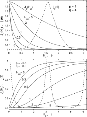
Figure 1: Angular dependence of the critical current density $j_{c}(\theta)$, Eq. (III), (dashed lines) for $p=1$, $q=4$ (top, the maximum of $j_{c}$ is at $\theta=\pi/2$) and for $p=-0.5$, $q=0.5$ (bottom, the maximum of $j_{c}$ is at $\theta=0$). The solid lines show the corresponding sheet currents $J_{c}(H_{z})$ at $H_{ax}=0$, Eq. (9), and at $H_{ax}=0.3$, $0.5$, $1$, $2$, $5$ from Eqs. (III), (9). The current density is measured in units of $j_{c}(0)$, while $J_{c}$ and $H_{z}$ are in units of $j_{c}(0)d$.

We now consider typical examples of the dependence $j_{c}(\theta)$. Let at $H_{ax}=0$ the following dependence $J_{c}(H_{z})$ be extracted from some experimental magneto-optics data:

$$J_{c}(H_{z})=J_{c}(H_{z},0)=j_{c}(0)d\left[1+p\,\exp\left(-{q\,H_{z}\over H_{cr}}\right)\right]\,,$$ (9)

where $H_{cr}=j_{c}(0)d/2$, while $j_{c}(0)$ and the dimensionless $p$ and $q$ are constants [$j_{c}(0)$ and $q>0$]. Using Eqs. (III), one can easily verify that the corresponding angular dependence of the critical current density takes the form:

$$j_{c}(\theta)=j_{c}(0)\left[1+p\,(1+q\,t)\exp(-q\,t)\right]\,,$$

$$\tan\theta=t^{-1}\left[1+p\,\exp(-q\,t)\right]\,,$$ (10)

where $t$ is a curve parameter with range $0\leq t\leq\infty$ equivalent to $\pi/2\geq\theta\geq 0$. This dependence $j_{c}(\theta)$ is presented in Fig. 1 together with the function $J(H_{z})$, Eq. (9). Note that the character of this dependence $j_{c}(\theta)$ is typical of layered high-$T_{c}$ superconductors when $p>0$ and of superconductors with columnar defects when $p<0$. Using Eqs. (III) and (9), we find the dependences of $J_{c}$ on $H_{z}$ for $H_{ax}\neq 0$, Fig. 1. We consider now $H_{z}$ profiles for various types of pinning and for the different scenarios of switching on $H_{a}$.

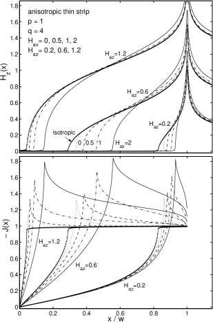
Figure 2: Spatial profiles of the perpendicular field component $H_{z}(x)$ (upper plot) and of the sheet current $J(x)$ (lower plot) of a thin strip with anisotropic pinning described by model (III) with $p=1$, $q=4$, see Fig. 1. $H_{ax}$ is switched on first and then $H_{az}$ (third scenario). The various curves correspond to increasing applied field $H_{az}=0.2$, $0.6$, $1.2$. The magnetic fields and the sheet current $J$ are in units of $j_{c}(0)d$. The dotted, dashed, dot-dashed, and solid curves are for $H_{ax}=0$, 0.5, 1, and 2, respectively. For comparison, the solid curves with dots (indicating the grid) show the profiles for isotropic pinning ($p=0$). The dotted lines also correspond to the opposite sequence of switching on $H_{az}$ and $H_{ax}$ (second scenario).

III.1 Layered superconductors, $p>0$

For layered superconductors ($p>0$), we begin our analysis with the third scenario when $H_{ax}$ is switched on first and then $H_{az}$ is applied. Appropriate magnetic-field profiles obtained with Eqs. (1), (2), (4) and $J_{c}(H_{z},H_{ax})$ of Fig. 1 are shown in Fig. 2. Note that for the third scenario one has $|J|=J_{c}$ at any point $x$ where $H_{z}(x)\neq 0$, and the penetration depth of $H_{z}$ into the strip, $w-a$, depends on $H_{ax}$. Another situation occurs when $H_{ax}$ and $H_{az}$ are switched on in the opposite sequence (the second scenario). After switching on $H_{az}$, the magnetic-field profiles are given by the dotted lines in Fig. 2. The subsequent increase of $H_{ax}$ does not change either $J(x)$ or $H_{z}(x)$. c Indeed, as seen from Fig. 1, $J_{c}(H_{z})$ increases with increasing $H_{ax}$. Hence, if $J(x)$ were equal to its critical value $J_{c}[H_{z}(x)]$, the penetration depth of the applied field $H_{az}$ would decrease as compared to $w-a$ for the dotted lines of Fig. 2, and flux lines near the points $x=\pm a$ would have to move against the Lorenz forces directed towards the center of the strip, which is impossible. Thus, for the second scenario the sheet current is less than its critical value for all points $x$. This means that although the fully penetrated critical state develops across the thickness of the strip in the regions penetrated by $H_{z}$, there is a boundary $z=z_{c}(x)$ at which the critical current density $j_{y}(x,z)$ changes its sign, Fig. 3, and so the magnitude of sheet current $|J|$ is less than $J_{c}$. It follows from Eq. (5) that the boundary $z_{c}(x)$ is determined by the formula,

$$2z_{c}(x)=-\!\!\int_{H_{x}^{-}}^{H_{x}^{+}}\!\!{dh\over j_{c}(h,H_{z})},$$ (11)

where $H_{x}^{-}=H_{ax}-0.5J(x)$, and $H_{x}^{+}=H_{ax}+0.5J(x)$ are the $x$ component of the magnetic field at the lower and the upper surfaces of the strip at the point $x$, while the sheet current $J(x)$ coincides with $J_{c}[H_{z}(x)]$ calculated at $H_{ax}=0$, i.e., $J(x)=-(x/|x|)J_{c}[H_{z}(x),0]$. Inserting the parametric form of $j_{c}(\theta)$, Eq. (III), into Eq. (11), we arrive at the following equations for $z_{c}$:

$${0.5J_{c}(H_{z},0)+H_{ax}\over H_{z}}={J_{c}(u_{+},0)\over 2u_{+}},$$

$${|0.5J_{c}(H_{z},0)-H_{ax}|\over H_{z}}={J_{c}(u_{-},0)\over 2u_{-}},$$

$${2z_{c}(x)\over d}={{\rm sgn}(x)H_{z}\over 2}\left({1\over u_{+}}+\sigma{1\over u_{-}}\right).$$ (12)

Here $u_{+}$ and $u_{-}$ are auxiliary variables; $\sigma$ is the sign of $[0.5J_{c}(H_{z},0)-H_{ax}]$; $H_{z}=H_{z}(x)$ is the magnetic-field profile at $H_{ax}=0$, and ${\rm sgn}(x)=\pm 1$ for $x>0$ and $x<0$, respectively.

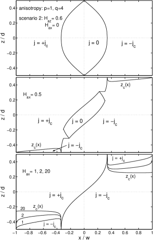
Figure 3: Current fronts and flux-free core in a thin strip with anisotropic pinning described by model (III) with $p=1$, $q=4$. The perpendicular magnetic field $H_{az}=0.6$ is applied first and then the in-plane component $H_{ax}$ is increased from zero to $H_{ax}=0.5$, $1$, $2$, $20$ (second scenario). At $|x|\leq a=0.339w$, the flux-free core and the lines separating the regions of the strip with opposite directions of currents are plotted, using c4 the results of Ref. mbi, . The new boundary $z=z_{c}(x)$ which occurs at $a\leq|x|\leq w$ is calculated from Eqs. (III.1). This boundary remains practically unchanged when $H_{ax}\geq 8$. The magnetic fields are measured in units of $j_{c}(0)d$.

For the first scenario of switching on $H_{a}$ when $H_{az}$ and $H_{ax}$ increase simultaneously, the magnetic-field profiles calculated for the same final values of $H_{az}$ and $H_{ax}$ as in Fig. 2 coincide with the profiles for the third scenario shown in this figure.

III.2 Superconductors with columnar defects, $p<0$

Consider now a superconductor with columnar defects directed along the $z$ axis. To model the sheet current $J(H_{z})$ in such superconductors, one can use Eq. (9) with $p<0$, Fig. 1. In Fig. 4 we present the appropriate magnetic-field profiles. Note that these profiles coincide for the three scenarios of switching on $H_{a}$ (neglecting the effect of flux creep which can be different for different scenarios). However, the profiles and the penetration depth of $H_{z}$ depend on $H_{ax}$. When $H_{ax}$ increases, the profiles tend to those of superconductors without columnar defects [it is evident from Fig. 1 that pinning without these defects is implied to be isotropic and to be described by the Bean model with constant $j_{c}(\theta)=j_{c}(\pi/2)$]. The change of the profiles occurs in a rather narrow interval of $H_{ax}$. This result can be understood from the following simple considerations: Although the columnar defects increase pinning in the strip, this increase occurs mainly when the angle $\theta$ of a flux line does not exceed the so-called trapping angle $\theta_{t}$. bl It is this $\theta_{t}$ that determines the width of the peak in $j_{c}(\theta)$ caused by the defects. When $H_{ax}$ increases, the characteristic tilt of the flux lines in the strip, $H_{ax}/H_{z}$, also increases, and when the tilt exceeds $\theta_{t}$, pinning by the columnar defects becomes ineffective.

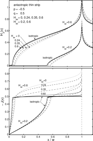
Figure 4: Spatial profiles of the perpendicular field component $H_{z}(x)$ (upper plot) and of the sheet current $J(x)$ (lower plot) of a thin strip with anisotropic pinning described by model (III) with $p=-0.5$, $q=0.5$, see Fig. 1. The various curves correspond to increasing applied field $H_{az}=0.2$, $0.6$. The magnetic fields and the sheet current $J$ are in units of $j_{c}(0)d$. The dotted, dashed, dot-dashed, and solid curves are for $H_{ax}=0$, $0.24$, $0.35$, and $0.6$, respectively. At any $H_{ax}>0.6$ the profiles practically coincide with those at $H_{ax}=0.6$, while at $H_{ax}<0.2$ the profiles are very close to that at $H_{ax}=0$. The profiles at $H_{ax}=0.6$ also almost coincide with the profiles for isotropic pinning with $j_{c}(\theta)=j_{c}(\pi/2)$ (solid curves with dots indicating the used grid). The profiles $H_{z}(x)$ and $J(x)$ coincide for the three scenarios of switching on $H_{a}$.

IV How to reconstruct $j_{c}$ from $H_{z}(x)$

We now discuss the problem of the reconstruction of $j_{c}({\bf H})$ from experimental magnetic-field profiles. Various procedures were elaborated R ; JH ; Gr ; W ; J ; G ; Joo ; Kr which enable one to extract the spatial distribution of the sheet current $J$ from an experimental $H_{z}$ profile measured at the upper surface of a thin flat superconductor. In particular, for the case of the strip, equation (1) can be explicitly inverted:JH

$$J(x)={2\over\pi}\int_{-w}^{w}\!\!{H_{z}(v)-H_{az}\over v-x}\left({w^{2}-v^{2}\over w^{2}-x^{2}}\right)^{1/2}dv.$$ (13)

Eliminating $x$ from $H_{z}(x)$ and $J(x)$ (in the region of a nonzero $H_{z}$), one can find the function $J_{c}(H_{z})$ from experimental data; see, e.g., Ref. ita, .

If the extracted $J_{c}(H_{z})\approx\$const., this means that the Bean model is valid, and $j_{c}=J_{c}/d$. It is this formula that is commonly used to find $j_{c}$ in experiments. However, this simple approach in general is not correct when $J_{c}$ depends on $H_{z}$. It is necessary to distinguish between two situations. For the case of weak collective pinning by point defects in the small bundle pinning regime, $j_{c}$ depends only on the combination $|H|\cos\theta=H_{z}$. bl Then, the critical current density is constant across the thickness of the strip, and one still has

$$j_{c}(H_{z})={J_{c}(H_{z})\over d},$$ (14)

i.e., the usual formula is valid. On the other hand, when $j_{c}$ depends on $\theta$ and $|H|$ separately, and when to the first approximation one can assume that $j_{c}=j_{c}(\theta)$ (see Sec. III), formulas (III) should be used to reconstruct the $j_{c}(\theta)$ from $J_{c}(H_{z})$ obtained at $H_{ax}=0$. In order to distinguish between these two situations, i.e., to choose between formulas (III) and (14), one can use the magnetic field profiles obtained in oblique magnetic fields.

When $j_{c}=j_{c}(H_{z})$, the magnetic-field profiles in oblique magnetic fields depend only on $H_{az}$ and are the same for any scenario of switching on ${\bf H}_{a}$. On the other hand, the results of Sec. III show that another situation occurs when $j_{c}$ is not only a function of $H_{z}$. In this case the penetration depth of $H_{z}$ depends on $H_{ax}$. Moreover, different scenarios can lead to different profiles $H_{z}(x)$.

When the magnetic-field profiles in oblique magnetic fields show that the dependence $j_{c}=j_{c}(H_{z})$ cannot explain the experimental data, one can apply formulas (III) to extract $j_{c}(\theta)$ from the $H_{z}$ profiles at $H_{ax}=0$. If the sample is not too thick, $j_{c}d<H_{0}$, where $H_{0}$ is the characteristic scale of the $|H|$-dependence of $j_{c}$, the extracted $j_{c}(\theta)$ approximately gives $j_{c}(\theta,H=0)$. For thicker samples the obtained $j_{c}(\theta)$ can be considered as a first step in determining $j_{c}(\theta,|H|)$. Calculating then the magnetic field profiles in oblique fields and comparing them with appropriate experimental data, one can verify the assumption $j_{c}=j_{c}(\theta)$ (i.e., the fulfilment of $j_{c}d<H_{0}$) for the superconductor under study. If this assumption does not lead to a good agreement with the data in oblique magnetic fields, one should supplement the obtained $j_{c}(\theta)$ with some $|H|$ dependence. We emphasize that since the function $J_{c}(H_{z},H_{ax})$ extracted from the magnetic-field profiles in oblique magnetic fields, depends on two variables $H_{z}$ and $H_{ax}$, this function, in principle, enables one to determine $j_{c}(\theta,|H|)$ depending on two variables, too. However, in this determination one should first assume some model of the ${\bf H}$-dependence of $j_{c}$ and then calculate $J_{c}(H_{z},H_{ax})$ from Eq. (6); see, e.g., Appendix A. On the other hand, when $j_{c}d<H_{0}$, formulas (III) give the model-independent $j_{c}(\theta,0)$ directly from the experimental data.

Appendix A $j_{c}$ depends on $\theta$ and $H_{z}$

Here we present some formulas for reconstruction of $j_{c}({\bf H})$ when the simplest form $j_{c}=j_{c}(\theta)$ cannot sufficiently well describe the experimental magnetic-field profiles in perpendicular and oblique magnetic fields. We assume that $j_{c}({\bf H})$ can be presented in the form: $j_{c}({\bf H})=j_{c}(\theta)/f(H_{z})$ where the function $f(H_{z})$ takes into account a possible dependence of $j_{c}$ on $|H|$. B1

Let the functions $J_{c}(H_{z},0)\equiv J_{c}(H_{z})$ and $J_{c}(H_{z},H_{ax})$ be extracted from the magnetic-field profiles obtained for the perpendicular and oblique magnetic fields, see Eq. (13). In other words, these functions are assumed to be known here. Then, repeating the analysis of Eq. (6) in Sec. III, we arrive at the equations:

$$j_{c}(\theta)d=\left(\!J_{c}(H_{z})-H_{z}{dJ_{c}(H_{z})\over dH_{z}}\right){H_{z}f(H_{z})\over F(H_{z})}\,,$$

$$\tan\theta={J_{c}(H_{z})\over 2H_{z}}\,,$$ (15)

$$\ln[f(H_{z})]=\int_{0}^{H_{z}}\!\!du\left({F(u)\over u^{2}}-{1\over u}\right)$$

that generalize the parametric representation of $j_{c}(\theta)$, Eqs. (III). Here the function $F(H_{z})$ is determined by the formula:

$${1\over F(H_{z})} = {1\over 2t_{+}}+\sigma{1\over 2t_{-}},$$ (16)

where $\sigma$ is the sign of $[0.5J_{c}(H_{z},H_{ax})-H_{ax}]$, and $t_{+}$, $t_{-}$ are found from the two uncoupled equations,

$${0.5J_{c}(H_{z},H_{ax})+H_{ax}\over H_{z}} = {J_{c}(t_{+},0)\over 2t_{+}},$$

$${|0.5J_{c}(H_{z},H_{ax})-H_{ax}|\over H_{z}} = {J_{c}(t_{-},0)\over 2t_{-}}.$$ (17)

When $F(H_{z})=H_{z}$, one has $f(H_{z})=1$, and Eqs. (A) reduce to Eq. (III). Note that the function $F(H_{z})$ obtained from Eqs. (16), (A) has to be practically independent of $H_{ax}$ for our assumption $j_{c}({\bf H})=j_{c}(\theta)/f(H_{z})$ to be justified.

References

- (1) Ch. Jooss, J. Albrecht, H. Kuhn, S. Leonhardt, and H. Kronmüller, Rep. Prog. Phys. 65, 651 (2002).
- (2) B. J. Roth, N. G. Sepulveda, J. P. Wikswo,Jr, J. Appl. Phys. 65, 361 (1989).
- (3) E. H. Brandt, Phys. Rev. B46, 8628 (1992).
- (4) P. D. Grant, M. V. Denhoff, W. Xing, P. Brown, S. Govorkov, J. C. Irwin, B. Heinrich, H. Zhou, A. A. Fife, A. R. Cragg, Physica C 229, 289 (1994).
- (5) R. J. Wijngaarden, H. J. W. Spoelder, R. Surdeanu, R. Griessen, Phys. Rev. B54, 6742 (1996).
- (6) T. H. Johansen, M. Baziljevich, H. Bratsberg, Y. Galperin, P. E. Lindelof, Y. Shen, P. Vase, Phys. Rev. B54, 16264 (1996).
- (7) A. E. Pashitski, A. Gurevich, A. A. Polyanskii, D. S. Larbalestier, A. Goyal, E. D. Specht, D. M. Kroeger, J. A. DeLuca, J. E. Tkaczyk, Science 275, 367 (1997).
- (8) Ch. Jooss, R. Warthmann, A. Forkl, H. Kronmüller, Physica C 299, 215 (1998).
- (9) F. Laviano, D. Botta, A. Chiodoni, R. Gerbaldo, G. Ghigo, L. Gozzelino, and E. Mezzetti, Phys. Rev. B68, 014507 (2003).
- (10) M. V. Indenbom, Th. Shuster, M. R. Koblischka, A. Forkl, H. Kronmüller, L. A. Dorosinskii, V. K. Vlasko-Vlasov, A. A. Polyanskii, R. L. Prozorov, V. I. Nikitenko, Physica C 209, 259 (1993).
- (11) M. R. Koblischka, R. J. Wijngaarden, Supercond. Sci. Technol. 8, 189 (1995).
- (12) E. Zeldov, D. Majer, M. Konczykowski, A. I. Larkin, V. M. Vinokur, V. B. Geshkenbein, N. Chikumoto, and H. Shtrikman, Europhys. Lett. 30, 367 (1995).
- (13) G. P. Mikitik, E. H. Brandt, M. Indenbom, Phys. Rev. B70, 014520 (2004).
- (14) In principle, the differences between these critical states can be detected via the component of the magnetic moment. mbi
- (15) G. P. Mikitik and E. H. Brandt, Phys. Rev. B62, 6800 (2000).
- (16) G. P. Mikitik and E. H. Brandt, Phys. Rev. B71, 012510 (2005).
- (17) G. Blatter, M. V. Feigel’man, V. B. Geshkenbein, A. I. Larkin, V. M. Vinokur, Rev. Mod. Phys. 66, 1125 (1994).
- (18) Equations (III) may be solved, e.g., by writing them in the form , , where are functions of the three independent variables , , and then minimizing numerically, starting with appropriate initial values. Using the solution at some , as the initial values for nearby , , one can find , , for any , , starting with the known solution at .
- (19) E. H. Brandt, Phys. Rev. B49, 9024 (1994); ibid 64, 024505 (2001).
- (20) Of course, in reality flux creep will change these and , causing decay of and thus deeper penetration of into the sample. However, these changes cannot mask the difference between the profiles for the second and third scenarios since this difference is of opposite sign, see Fig. 2.
- (21) The formulas of Ref. mbi, can describe the critical state of the strip in the core region even for the case since the flux lines are practically parallel to the strip plane there and . Hence, it is sufficient to put in the formulas of Ref. mbi, and to use obtained numerically from the solution of the critical state problem for the infinitely thin strip with the appropriate .
- (22) It is clear that a function of and can be represented as a function of and . However, the essential assumption is that is a product of factors depending on and .