Superconductivity-Induced Transfer of In-Plane Spectral Weight in Bi₂Sr₂CaCu₂O₈: Resolving a Controversy

Abstract

We present a detailed analysis of the superconductivity-induced redistribution of optical spectral weight in Bi₂Sr₂CaCu₂O₈ near optimal doping. It confirms the previous conclusion by Molegraaf et al. (Science 295, 2239 (2002)), that the integrated low-frequency spectral weight shows an extra increase below $T_{c}$. Since the region, where the change of the integrated spectral weight is not compensated, extends well above 2.5 eV, this increase is caused by the transfer of spectral weight from interband to intraband region and only partially by the narrowing of the intraband peak. We show that the opposite assertion by Boris et al. (Science 304, 708 (2004)), regarding this compound, is unlikely the consequence of any obvious discrepancies between the actual experimental data.

I Introduction

The problem of the superconductivity (SC) induced spectral weight (SW) transfer in the high-$T_{c}$ cuprates is in the focus of numerous experimental MolegraafScience02 ; SantanderEPL03 ; BorisScience04 ; SchuetzmannPRB97 ; MolerScience98 ; TsvetkovNature98 ; KirtleyPRL99 ; GaifullinPRL99 ; BasovScience99 ; BorisPRL02 ; KuzmenkoPRL03 ; MarelKluwer04 ; DeutscherCM05 and theoretical HirschPC92 ; AndersonScience95 ; LeggettScience96 ; ChakravartyEPJB98 ; ChakravartyPRL99 ; MunzarPRB01 ; MunzarPRB03 ; NormanPRB02 ; MarelKluwer03 ; KnigavkoPRB04 ; AbanovPRB04 ; BenfattoEPJB04 ; AndersonJPCM04 ; HirschPRB04 ; StanescuPRB04 ; MaierPRL04 ; FaridPM04 studies. Molegraaf et al. MolegraafScience02 reported the SC induced increase of the intraband spectral weight in optimally doped ($T_{c}$ = 88 K) and underdoped ($T_{c}$ = 66 K) single crystals of Bi₂Sr₂CaCu₂O₈ (Bi2212) based on combined ellipsometry and reflectivity measurements. Santander-Syro et al. SantanderEPL03 independently arrived at the same conclusions by analyzing reflectivity spectra of high-quality Bi2212 films. However, these results were recently questioned by Boris et al. BorisScience04 , who reported fully ellipsometric measurements of optimally doped YBa₂Cu₃O_6.9 (Y123, $T_{c}$ = 92.7 K) and slightly underdoped Bi2212 ($T_{c}$ = 86 K) and concluded that in these two materials there is ’a sizable superconductivity-induced decrease of the total intraband spectral weight’. It is thus necessary to clarify this experimental controversy.

The following reasons can potentially cause the opposite conclusions by different teams, namely: (i) non-identical compounds and doping levels were used, (ii) essentially different experimental results were obtained, or (iii) the analysis and interpretation of similar experimental data seriously deviate, most likely, in the way to determine the SC-caused change of the low-frequency SW:

$$W(\Omega_{c},T)=\rho_{s}(T)+\int_{0^{+}}^{\Omega_{c}}\sigma_{1}(\omega,T)d\omega,$$ (1)

where $\rho_{s}(T)$ is the spectral weight of the condensate, $\sigma_{1}(\omega,T)$ is the real part of the optical conductivity and the cutoff energy $\Omega_{c}$ represents the scale of scattering of the intraband (Drude) excitations.

Because of reason (i), we restrict our present discussion to the case of Bi2212 near optimal doping, which was studied by all mentioned teams BorisScience04 ; MolegraafScience02 ; SantanderEPL03 . We should keep in mind that, even with this restriction, the $T_{c}$’s and the stoichiometries of the samples are still not identical.

Regarding point (ii) we found that the experimental graphs, presented in Ref. BorisScience04, , do not significantly deviate from our earlier observations on optimally doped Bi2212 MolegraafScience02 . In particular, we show that the data on Bi2212, presented in Ref. BorisScience04, , given the error bars, do not challenge the previous conclusion about the SC-induced increase of $W(\Omega_{c},T)$ $(\Omega_{c}$ was 1.25 eV in Ref.MolegraafScience02, ).

This leaves possibility (iii) as the only remaining option: The contradicting conclusions of Ref. BorisScience04, and those of Refs. MolegraafScience02, ; SantanderEPL03, originate from a different analysis of the mutually non-contradicting experimental data. In the present paper we scrutinize the arguments of Ref. BorisScience04, and we point out an unjustified use of the Kramers-Kronig (KK) relations in interpreting their data, which appears to be responsible, at least in part, for the conclusions opposite to Refs. MolegraafScience02, and SantanderEPL03, .

The limited space of Ref.MolegraafScience02, did not allow explaining in depth the full analysis done. In this paper we present a more detailed and rigorous analysis of the experimental data published in Ref.MolegraafScience02, and arrive at additional arguments supporting the original conclusions. In order to numerically decouple the superconductivity-induced changes of the optical properties from the temperature dependencies, already present in the normal state (such as a gradual narrowing of the Drude peak), we apply the slope-difference analysis, developed in Ref. KuzmenkoPRL03, , which is closely related to the well-known temperature-modulation technique Cardona69 ; HolcombPRL94 . It appears that any realistic model, which satisfactorily fits the total set of experimental data (reflectivity below 0.75 eV and ellipsometrically obtained real and imaginary parts of the dielectric function at higher energies), gives an increase of $W(\Omega_{c},T)$ below $T_{c}$. Moreover, all attempts to do the same fitting with an artificial constraint, that the SC-induced change of $W(\Omega_{c},T)$ is negative (as is claimed in Ref.BorisScience04, ), or even zero, failed to fit the data, despite using flexible multi-oscillator modelsKuzmenkoCM05 . Importantly, the ellipsometrically measured real and imaginary parts of the dielectric function, $\epsilon_{1}(\omega)$ and $\epsilon_{2}(\omega)$, at high frequencies provide the most stringent limits on the possible change of the low-frequency spectral weight $W(\Omega_{c},T)$, due to the KK relations.

Finally we discuss whether the SC-increase of $W(\Omega_{c},T)$ is caused by the extra narrowing of the Drude peak below $T_{c}$ or by removal of the SW from the interband region. Indeed we find an extra narrowing of the Drude peak, in agreement with Ref.BorisScience04, . However, this narrowing is too small to explain the increase of the low-frequency spectral weight, which suggests that there is a sizeable spectral weight transfer from the range of the interband transitions.

II Experimental consistency of the reported results

First of all, we need to check if there are any qualitative discrepancies between the results published in Ref.BorisScience04, and our data, which can immediately lead to the opposite conclusions. In Fig.1 we reproduce the difference curves $\Delta\epsilon_{1}(\omega)=\epsilon_{1}(\omega,100K)-\epsilon_{1}(\omega,20K)$ and optical conductivity $\Delta\sigma_{1}(\omega)=\sigma_{1}(\omega,100K)-\sigma_{1}(\omega,20K)$ for Bi2212 close to optimal doping from ellipsometric measurements of Ref.BorisScience04, (Fig. S5) together with the same curves, obtained by the KK transformation of the reflectivity spectra of Ref. MolegraafScience02, , re-plotted in the same fashion. Although for the purpose of comparison of spectra in this range we have to use the KK-transformed quantities, the main analysis which we present in sections IV and V of this paper is based on the directly measured optical quantities. We also point out right away, that these difference curves do not eliminate the normal-state temperature trends, unrelated to the SC phase transition. In sections IV and V we present what we believe to be the correct analysis, which takes into account the normal-state temperature dependence of optical properties.

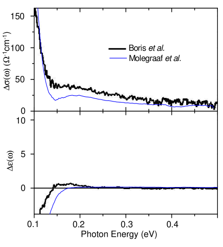
Figure 1: Differential dielectric function $\Delta\epsilon_{1}(\omega)=\epsilon_{1}(\omega,100K)-\epsilon_{1}(\omega,20K)$ and optical conductivity $\Delta\sigma_{1}(\omega)=\sigma_{1}(\omega,100K)-\sigma_{1}(\omega,20K)$ of Bi2212 near optimal doping, measured by ellipsometry in Ref.BorisScience04, (black curve) and derived by the KK transformation of reflectivity data from Ref. MolegraafScience02, (blue curve). The latter KK-transformed data are shown for comparison only; our analysis is based on the directly measured reflectivity in the infrared and ellipsometry above 0.75 eV.

One can state that there is a qualitative agreement between the $\Delta\epsilon_{1}(\omega)$ and $\Delta\sigma_{1}(\omega)$ curves of the two groups, especially considering that these difference curves are on a 10-fold amplified scale as compared to the spectra itself (Fig. 1 of Ref. MolegraafScience02, , Fig. S4 of Ref. BorisScience04, ) and a possible difference of the sample compositions.

Clearly, no model-independent argument, without specific calculations, can give opposite signs of the change of the SW, when applied to these two data sets. Therefore, the different conclusions of different teams are unlikely the consequence of any obvious discrepancies between the actual experimental data.

An important remark is that the scale and the data scatter on Fig.1 do not allow to distinguish the change of $\epsilon_{1}(\omega)$ from zero for frequencies between 0.2 and 0.5 eV. As a result, the authors of Ref.BorisScience04, base their argument on $\Delta\epsilon_{1}(\omega)$ being zero in this range. In contrast, later we show that it is small, but not zero, including the range above 0.5 eV. In fact, this observation will be extremely important to determine the sign of the SW change.

III On the role of the Kramers-Kronig relations

Since the optical conductivity $\sigma_{1}(\omega)$ is not directly measured down to zero frequency, the calculation of $W(\Omega_{c},T)$ requires, in principle, the extrapolation of data, using certain data modelling. It turns out, however, that the use of the Kramers-Kronig relation between $\epsilon_{1}(\omega)$ and $\sigma_{1}(\omega)$

$$\epsilon_{1}(\omega)-1=8\mathchoice{{\vbox{\hbox{$\textstyle-$}}\kern-4.86108pt}}{{\vbox{\hbox{$\scriptstyle-$}}\kern-3.25pt}}{{\vbox{\hbox{$\scriptscriptstyle-$}}\kern-2.29166pt}}{{\vbox{\hbox{$\scriptscriptstyle-$}}\kern-1.875pt}}\!\int_{0}^{\infty}\frac{\sigma_{1}(x)}{x^{2}-\omega^{2}}dx$$ (2)

helps to avoid unnecessary model assumptions and drastically decrease the resulting error bars.

The authors of Ref.BorisScience04, propose a model-independent argument in order to show that there is an overall decrease of the intraband spectral weight below $T_{c}$. The argument is based on two of their experimental observationssignconvention : (i) $\Delta\sigma_{1}(\omega)>0$ between $\omega_{1}$ = 0.15 eV and $\omega_{2}$ = 1.5 eV, (ii) $\Delta\epsilon_{1}(\omega)=0$ in the same energy region. We reproduce partially their statement here: ”The SW loss between 0.15 eV and 1.5 eV then needs to be balanced by a corresponding SW gain below 0.15 eV and above 1.5 eV. In other words, there is necessarily a corresponding SW gain in the interband energy range above 1.5 eV caused by a decrease of the total intraband SW.”

We believe that this statement is incorrect. The justification given by the authors of Ref.BorisScience04, considers a weaker set of conditions: $\Delta\sigma_{1}(\omega)>0$ for $\omega_{1}<\omega<\omega_{2}$, and $\Delta\epsilon_{1}(\omega_{0})=0$ at one particular frequency $\omega_{0}$ between $\omega_{1}$ and $\omega_{2}$. We rewrite Equation (S3) of Ref. BorisScience04, in the form:

$$-\int_{0}^{\omega_{1}}\frac{\Delta\sigma_{1}(x)}{\left|x^{2}-\omega_{0}^{2}\right|}+\mathchoice{{\vbox{\hbox{$\textstyle-$}}\kern-4.86108pt}}{{\vbox{\hbox{$\scriptstyle-$}}\kern-3.25pt}}{{\vbox{\hbox{$\scriptscriptstyle-$}}\kern-2.29166pt}}{{\vbox{\hbox{$\scriptscriptstyle-$}}\kern-1.875pt}}\!\int_{\omega_{1}}^{\omega_{2}}\frac{\Delta\sigma_{1}(x)}{x^{2}-\omega_{0}^{2}}$$

$$+\int_{\omega_{2}}^{\infty}\frac{\Delta\sigma_{1}(x)}{\left|x^{2}-\omega_{0}^{2}\right|}=-A+B+C=0.$$ (3)

Now we note, that even though $\Delta\sigma_{1}$ in the integral $B$ is positive, the value of $B$ can have either sign. It means that there is formally no limitation on the sign of $C-A$, nor on the signs of $A$ and $C$ separately. Appealing to the general $f$-sum rule $\int_{0}^{\infty}\Delta\sigma_{1}(x)dx=0$ does not remove the uncertainty, because the change of the low-frequency spectral weight can be, in principle, compensated at arbitrarily high frequencies, which give an arbitrarily small contribution to the KK integral.

The stronger condition that $\Delta\epsilon_{1}(\omega)$ is exactly zero for $\omega_{1}<\omega<\omega_{2}$ is physically pathological and it appears to be more difficult to address mathematically. It was not explained in Ref.BorisScience04, how this condition leads to the cited statement. Furthermore, we observe that $\Delta\epsilon_{1}(\omega)$ is actually not zero in this range. We thus disagree with the model-independent argument in favor of the SC-induced decrease of the charge carrier SW, as is claimed in Ref.BorisScience04, .

On the other hand, we absolutely agree with Ref.BorisScience04, , that the KK relations between $\epsilon_{1}(\omega)$ and $\sigma_{1}(\omega)$ must stay as an important ingredient of the data analysis Text1 . However, in our opinion trustworthy conclusions can only be drawn from a thorough numerical treatment of the full set of available optical data. Importantly, due to the KK relations, the behavior of $\epsilon_{1}(\omega,T)$ and $\epsilon_{2}(\omega,T)$ at high frequencies appears to be the most sensitive indicator of the spectral weight transfer. We present such an analysis in the following sections.

IV Superconductivity-related spectral changes

As described in Ref.MolegraafScience02, , the normal-incidence reflectivity $R(\omega)$ was measured between 200 and 6000 cm^-1 (25 meV - 0.75 eV) and real and imaginary parts of dielectric function $\epsilon_{1}(\omega)$ and $\epsilon_{2}(\omega)$, were obtained by spectroscopic ellipsometry from 6000 to 36000 cm^-1 (0.75 - 4.5 eV).

In Figs. 2, 3 we display the temperature dependence of reflectivity, and $\epsilon_{1,2}(\omega,T)$ respectively, for selected photon energies. The complex dielectric constant changes as a function of temperature in the entire range from 0 to 300 K. For frequencies larger than 0.25 eV the variation as a function of temperature is essentially proportional to $T^{2}$. The same temperature dependence has been observed in other cuprate superconductors, for exampleortolani05 La_2-xSr_xCuO₄, and has been explained quantitatively using the Hubbard modelToschiCM05 . For frequencies below 0.1 eV the optical conductivity has a very large intraband-contribution, with a linearly increasing dissipation, which causes a non-monotonous temperature dependence of $\epsilon_{1}$ and $\epsilon_{2}$. In particular, it was found MarelNature03 that the $1/(T\sigma_{1}(\omega))$ is equal to a constant plus a term proportional to $T^{-2}$. The gradual decrease of the high-frequency conductivity with cooling down is also expected due to the reduction of the electron-phonon scatteringKarakozovSSC02 .

The onset of the superconductivity is marked by clear kinks (slope changes) at $T_{c}$ of the measured optical quantities (Fig.2, 2). An exciting feature of the high-$T_{c}$ cuprates is that the kinks are seen not only in the region of the SC gap, but also at much higher photon energies (at least up to 2.5 eV in Ref. MolegraafScience02, ). It means that the formation of the SC long-range order causes a redistribution of the spectral weight across a very large spectral range; a fact, which several groups agree upon BorisScience04 ; MolegraafScience02 ; SantanderEPL03 ; RuebhausenPRB01 ; HolcombPRL94 .

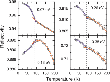
Figure 2: Temperature dependent reflectivity of Bi2212 close to optimal doping ($T_{c}$= 88 K) for selected frequencies in the infrared range. The blue (red) curves are polynomial fits to the temperature dependence below (above) $T_{c}$, used to produce the kink (slope difference) values.

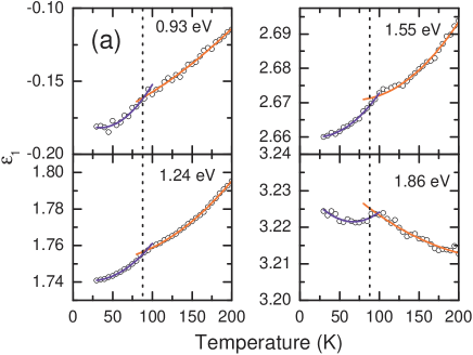
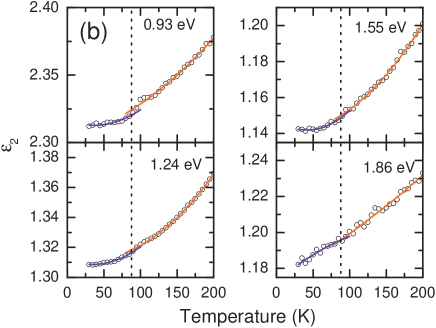
Figure 3: Temperature dependent ellipsometrically measured $\epsilon_{1}(T)$ (a) and $\epsilon_{2}(T)$ (b) of Bi2212 close to optimal doping ($T_{c}$= 88 K) for selected frequencies. The blue (red) curves are polynomial fits to the temperature dependence below (above) $T_{c}$, used to produce the kink (slope change) values. Not all temperature datapoints are shown.

An essential aspect of the data analysis is the way to separate the superconductivity-induced changes of the optical constants from the temperature-dependent trends, observed above $T_{c}$. A similar problem is faced in the specific-heat experiments JunodPC99 ; LoramJPCS01 , where the superconductivity-related structures are superimposed on a strong temperature dependent background. Let us introduce a slope-difference operator $\Delta_{s}$, which measures the slope change (kink) at $T_{c}$KuzmenkoPRL03 :

$$\Delta_{s}f(\omega)\equiv\left.\frac{\partial f(\omega,T)}{\partial T}\right|_{T_{c}+\delta}-\left.\frac{\partial f(\omega,T)}{\partial T}\right|_{T_{c}-\delta},$$ (4)

where $f$ stands for any optical quantity. It properly quantifies the effect of the SC transition, since the normal state trends are cancelled outfootnotekink . Since $\Delta_{s}$ is linear, the slope-difference KK relation is also valid:

$$\Delta_{s}\epsilon_{1}(\omega)=8\mathchoice{{\vbox{\hbox{$\textstyle-$}}\kern-4.86108pt}}{{\vbox{\hbox{$\scriptstyle-$}}\kern-3.25pt}}{{\vbox{\hbox{$\scriptscriptstyle-$}}\kern-2.29166pt}}{{\vbox{\hbox{$\scriptscriptstyle-$}}\kern-1.875pt}}\!\int_{0}^{\infty}\frac{\Delta_{s}\sigma_{1}(x)}{x^{2}-\omega^{2}}dx.$$ (5)

In order to detect and measure a kink as a function of temperature as well as to establish whether or not the kink is seen at $T_{c}$  the spectra must be measured using a fine temperature resolution. A resolution of 2 K or better was used in the entire range from 10 to 300 K, enables us to perform a reliable slope-difference analysis.

The datapoints in Figs. 4a and 4b show $\Delta_{s}R(\omega)$ and $\Delta_{s}\epsilon_{1}(\omega)$ and $\Delta_{s}\epsilon_{2}(\omega)$, obtained from the directly measured temperature-dependent curves shown in Fig. 2 and 3. The details of the corresponding numerical procedure and the determination of the error bars are described in Appendix A1.

One can see, that $\Delta_{s}\epsilon_{1}(\omega)$ is negative and its absolute value is strongly decreasing as a function of frequency. In the same region, $\Delta_{s}\epsilon_{2}(\omega)$ is almost zero (within our error bars). Intuitively, it already suggests that the low-frequency integrated spectral weight $W(\Omega_{c},T)$ is likely to increase in the SC state. Indeed, in the simplest scenario, when the extra SW is added at zero frequency, one has $\Delta_{s}\epsilon_{1}(\omega)=-8\Delta_{s}W(0+)\omega^{-2}$. This formula becomes approximate, if changes also take place at finite frequencies. However, the approximation is good, if the most significant changes $\Delta_{s}\sigma_{1}$ occur only below $\omega_{1}\ll\omega$, and above $\omega_{2}\gg\omega$. This follows from the exact expansionBozovicPRB90 of Eq. 5, valid for $\omega_{1}<\omega<\omega_{2}$:

$$\Delta_{s}\epsilon_{1}(\omega)=-\sum_{j=0}^{\infty}\frac{A_{j}}{\omega^{2+2j}}+\Delta_{s}\tilde{\epsilon}_{1}(\omega)+\sum_{j=0}^{\infty}B_{j}\omega^{2j},$$ (6)

where

$$A_{j} \equiv 8\int_{0}^{\omega_{1}}x^{2j}\Delta_{s}\sigma_{1}(x)dx$$

$$B_{j} \equiv 8\int_{\omega_{2}}^{\infty}\frac{\Delta_{s}\sigma_{1}(x)}{x^{2+2j}}dx$$

$$\Delta_{s}\tilde{\epsilon}_{1}(\omega) \equiv 8\mathchoice{{\vbox{\hbox{$\textstyle-$}}\kern-4.86108pt}}{{\vbox{\hbox{$\scriptstyle-$}}\kern-3.25pt}}{{\vbox{\hbox{$\scriptscriptstyle-$}}\kern-2.29166pt}}{{\vbox{\hbox{$\scriptscriptstyle-$}}\kern-1.875pt}}\!\int_{\omega_{1}}^{\omega_{2}}\frac{\Delta_{s}\sigma_{1}(x)}{x^{2}-\omega^{2}}dx.$$

For $\omega_{1}$ = 0.8 eV and $\omega_{2}$ = 2.5 eV we can calculate $\Delta_{s}\tilde{\epsilon}_{1}(\omega)$ directly from the measured $\Delta_{s}\sigma_{1}(\omega)$. It turns out, that $\left|\Delta_{s}\tilde{\epsilon}_{1}(\omega)\right|$ $<$ 10^-4 K^-1, while the average value is indistinguishable from zero. In this situation we can neglect $\Delta_{s}\tilde{\epsilon}_{1}(\omega)$, compared to the contributions from the low and high frequencies. Thus, to leading order

$$\Delta_{s}\epsilon_{1}(\omega) \approx -A_{0}\omega^{-2}+B_{0}$$ (7)

$$= -8\Delta_{s}W(\omega_{1})\omega^{-2}+\Delta_{s}\epsilon_{\infty},$$

where $\epsilon_{\infty}=8\int_{\omega_{2}}^{\infty}\sigma_{1}(\omega)\omega^{-2}d\omega$ is the integrated oscillator strength of all optical excitations above $\omega_{2}$.

The best fit of $\Delta_{s}\epsilon_{1}(\omega)$ in the spectral region (0.8 - 2.5 eV) with Eq. 7 is shown by the green dashed line in Fig.4b. It gives $\Delta_{s}W(\Omega_{c})$ $\approx$ +360 $\Omega^{-1}$cm^-2K^-1 and $\Delta_{s}\epsilon_{\infty}$$\approx$ -10^-4 K^-1. Although these absolute values are very approximate, the signs of both parameters indicate that the spectral weight is taken from the region above 2.5 eV and added to the region below 0.8 eV.

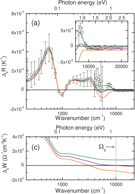
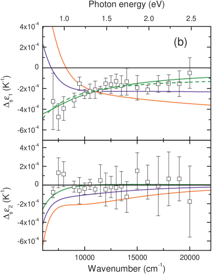
Figure 4: The spectral dependence of slope-difference $\Delta_{s}R(\omega)$ (a) and $\Delta_{s}\epsilon_{1,2}(\omega)$ and $\Delta_{s}\epsilon_{2}(\omega)$ (b). Datapoints show the kink value, derived from the temperature-dependent curves (Figs.2 and 3) as described in Appendix A1. Only few datapoints of $\Delta_{s}R(\omega)$ out of all used in the analysis are shown. Solid curves show different fits, as described in the text. The green curve indicates the best fit of $\Delta_{s}R(\omega)$, $\Delta_{s}\epsilon_{1}(\omega)$ and $\Delta_{s}\epsilon_{2}(\omega)$ simultaneously, giving $\Delta_{s}W(\Omega_{c})$ $\approx$ +770 $\Omega^{-1}$cm^-2K^-1 (the SC-induced increase of $W(\Omega_{c})$). The blue and red curves are the best fits of the same data with an artificial constraint $\Delta_{s}W(\Omega_{c})$ = 0 and -770 $\Omega^{-1}$cm^-2K^-1 respectively. One can see that both constraints are incompatible with the data. The green dashed line is the best fit of $\Delta_{s}\epsilon_{1}(\omega)$ by the formula $-A\omega^{-2}+B$. The integrated spectral weight $\Delta_{s}W(\omega)$ (c) for all three fits is shown by the same colors. The inset of panel (a) shows $\Delta_{s}R(\omega)$ calculated from the ellipsometrically measured dielectric function from 0.75 to 2.75 eV on an expanded vertical scale.

V Slope-difference spectral analysis

Now we present the full data analysis without using the approximation (7). The technique we present here is a modification of the temperature-modulation spectroscopyCardona69 ; HolcombPRL94 ; DolgovPC94 . Because of the KK relation (5), we can model the slope-difference dielectric function with the following dispersion formula: $\Delta_{s}\epsilon(\omega)$:

$$\Delta_{s}\epsilon(\omega)=\Delta_{s}\epsilon_{\infty}+\sum_{i=0}^{N}\frac{A_{i}}{\omega_{i}^{2}-\omega^{2}-i\gamma_{i}\omega}.$$ (8)

$\Delta_{s}\epsilon_{\infty}$ is responsible for the high-frequency electronic excitations, while each Lorentzian term represents either an addition or a removal of spectral weight, depending on the sign of $A_{i}$. We emphasize that this model is just a parametrization. The number of oscillators $N$ has to be chosen in order to get a good fit of experimental data. The physical meaning of some oscillators, taken alone, may not be well-defined. However, the essential feature of the functional form (8) is that it preservesText6 the KK relation (5).

We include the infrared $\Delta_{s}R(\omega)$ to the fitting procedure by making use of the following relationKuzmenkoPRL03 ; DolgovPC94 :

$$\Delta_{s}R(\omega)=\frac{\partial R}{\partial\epsilon_{1}}(\omega,T_{c})\Delta_{s}\epsilon_{1}(\omega)+\frac{\partial R}{\partial\epsilon_{2}}(\omega,T_{c})\Delta_{s}\epsilon_{2}(\omega)$$

$$=2R(\omega,T_{c})\mbox{ Re}\left[\frac{\Delta_{s}\epsilon(\omega)}{\sqrt{\epsilon(\omega,T_{c})}\left(\epsilon(\omega,T_{c})-1\right)}\right].$$ (9)

The method which we use to determine the ’sensitivity functions’ $(\partial R/\partial\epsilon_{1,2})(\omega,T_{c})$ from the experimental data is described in Appendix A2.

The green solid line in Fig.4a and 4b denotes the best fitREFFIT of $\Delta_{s}\epsilon_{1}(\omega)$ and $\Delta_{s}\epsilon_{2}(\omega)$ and, simultaneously, $\Delta_{s}R(\omega)$. One can see that all essential spectral details are well reproduced. The corresponding parameter values are collected in Table 1. The first term in (8) combines the condensate and the narrow ($\gamma$ $<$ 100 cm^-1) quasi-particle peak, while the remaining oscillators mimic the redistribution of spectral weight at finite frequencies.

Table 1: Model parameters of $\Delta_{s}\epsilon(\omega)$ by formula (8) which correspond to the best fit of the experimental data. $\Delta_{s}\epsilon_{\infty}$ = -3.1$\cdot$10^-5 K^-1.

$i$	$\omega_{i}$ (cm-1)	$A_{i}$ (105 cm-2K-1)	$\gamma_{i}$ (cm-1)
0	0	2.82	0
1	0	-11.25	3977
2	582	-2.40	488
3	939	2.20	707
4	2078	6.51	4496
5	2082	2.60	6141
6	3543	-0.17	1685

The slope-difference integrated spectral weight for the model (8):

$$\Delta_{s}W(\omega)=\frac{A_{0}}{8}+\int_{0+}^{\omega}\Delta_{s}\sigma_{1}(x)dx$$ (10)

is presented as a green curve in Fig.4c. It gives $\Delta_{s}W(\Omega_{c})$ $\approx$ +770 $\Omega^{-1}$cm^-2K^-1, which is about two times larger than the rough estimate in Section IV.

In order to test how robust this result is, we did two more fits of the same data, with an extra imposed constraint, that either (i) $\Delta_{s}W(\Omega_{c})$ = 0, or (ii) $\Delta_{s}W(\Omega_{c})$ = -770 $\Omega^{-1}$cm^-2K^-1. The resulting ’best-fitting’ curves are shown in Fig.4a, 4b and 4c in blue and red, respectively. One can clearly see that the models with $\Delta_{s}W(\Omega_{c})\leq 0$ fail to reproduce the experimental spectra, most spectacularly the high-frequency spectrum of $\Delta_{s}\epsilon_{1}(\omega)$. This is not surprising, since the imposed constraint changes the sign of the leading term $\sim\omega^{-2}$ in formula (7).

To exclude the possibility that the failure to get a good fit with the mentioned constraint would be a spurious result caused by the limited number of Lorentz oscillators used for fitting the data, we have also used the KK-constrained variational dielectric modelKuzmenkoCM05 , which is, in simple terms, a collection of a large number of adjustable oscillators, uniformly distributed in the whole spectral range, including the region above 2.5 eV. Thus we are confident that the dispersion model is able to reproduce all significant spectral features of the true function $\Delta_{s}\epsilon_{1}(\omega)$. However, these efforts did not improve the quality of the fit.

From this analysis we conclude that our experimental data unequivocally reveal the superconductivity-induced increase of $W(\Omega_{c},T)$ in optimally doped Bi2212, confirming the statements given in Refs.MolegraafScience02, ; SantanderEPL03, .

An alternative approach is to fit the total set of spectra at every temperatureMolegraafScience02 ; HajoThesis using a certain KK-consistent model with temperature-dependent parameters. There is a variety of possibilities to parameterize the dielectric function. However, it was shown by one of usHajoThesis that every model which reproduces satisfactorily not only the spectral features, but also the temperature dependence of the directly measured $R(\omega)$ and $\epsilon(\omega)$, gives a net increase of the low-frequency spectral weight below $T_{c}$.

VI Discussion

VI.1 Absolute change of the spectral weight

Having found that the integrated spectral weight $W(\Omega_{c},T)$ exhibits an extra increase below $T_{c}$, we want to evaluate its absolute superconductivity-induced change, continued into the low-temperature regionsignconvention :

$$\Delta W(\Omega_{c},T)\equiv W(\Omega_{c},T)-W_{n}(\Omega_{c},T),$$ (11)

where $W_{n}(\Omega_{c},T)$ is the ’correct’ extrapolation of the normal-state curve below $T_{c}$. In principle, $W_{n}(\Omega_{c},T)$ can be measured, when the superconducting order parameter is suppressed by an extremely high magnetic field (of the order of hundred Teslas). Unfortunately, such large fields are currently prohibitive for accurate optical experiments.

However, an order-of-magnitude estimate and, simultaneously, an upper limit of $\Delta W(\Omega_{c},T)$ at zero temperature can be obtained by the formula

$$\Delta W(\Omega_{c},0)\sim T_{c}\Delta_{s}W(\Omega_{c}).$$ (12)

This gives $\Delta W(\Omega_{c},0K)\sim 7\cdot 10^{4}\ \Omega^{-1}$cm^-2, which is about 1% of the total low-frequency spectral weight $W(\Omega_{c},0K)$$\approx$ 7 $\cdot$ 10⁶ $\Omega^{-1}$cm^-2. Since the temperature dependence of $\Delta W(\Omega_{c},T)$ is expected to saturate somewhat below $T_{c}$, a more realistic estimate is smaller by about a factor of 2 to 5, i.e. between 0.2 and 0.5% of $W(\Omega_{c},0K)$. These rough margins are suggested by the temperature dependence of the ab-planeLeePRL96 and c-axisGaifullinPRL99 penetration depths. Although this is a relatively small fraction, it is nevertheless significantMolegraafScience02 in the context of the theories where the superconducting transition is driven by the lowering of the kinetic energy HirschPC92 ; AndersonScience95 .

VI.2 The origin of the spectral weight transfer

The low-frequency integrated spectral weight $W(\Omega_{c},T)$ should not be confused with the intraband spectral weight:

$$W_{intra}(T)=\rho_{s}(T)+\int_{0+}^{\infty}\sigma_{1,intra}(\omega,T)d\omega,$$ (13)

where $\sigma_{1,intra}(\omega,T)$ is the conductivity due to intraband transitions. A legitimate question is whether the observed increase of $W(\Omega_{c},T)$ below $T_{c}$ is due to the transfer of SW from the interband transitions to the intraband (Drude) conductivity i. e., by the increase of $W_{intra}(T)$, or is simply caused by an extra narrowing of the Drude peak in the SC stateBorisScience04 ; KarakozovSSC02 , without changing $W_{intra}(T)$. The distinction between the intraband and interband spectral weights can be made in theoretical models, but in experimental spectra their separation is not unique, because of the unavoidable overlap between these spectral ranges. Nevertheless, the temperature and spectral behavior of the optical constants suggests a likely scenario.

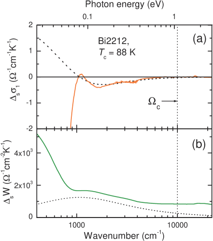
Figure 5: (a) Slope-difference conductivity $\Delta_{s}\sigma_{1}(\omega)$ of optimally doped Bi2212. (b) The corresponding integrated spectral weight $\Delta_{s}W(\omega)$. Dotted lines show a model, which mimics the narrowing of the Drude peak.

Fig.5a shows the slope-difference conductivity $\Delta_{s}\sigma_{1}(\omega)$, which is obtained by the most detailed multi-oscillator fitKuzmenkoCM05 of the data, shown in Fig.4. The decrease of $\sigma_{1}(\omega)$ below $T_{c}$ in the frequency range from 0.15 to about 0.8 eV is due to an extra narrowing of the Drude peak, caused by the reduced charge carrier scattering in the superconducting state. In the most crude model where the intraband peak is described by the Drude formula $\sigma_{1}(\omega)=(4\pi)^{-1}\omega_{p}^{2}\gamma(\omega^{2}+\gamma^{2})^{-1}$ and the superconductivity-induced narrowing is given by a simple change of $\gamma$, we get $\Delta_{s}\sigma_{1}(\omega)=(4\pi)^{-1}\omega_{p}^{2}(\omega^{2}-\gamma^{2})(\omega^{2}+\gamma^{2})^{-2}\Delta_{s}\gamma$. This shape (with $\gamma$ = 0.14 eV) matches the experimental curve above 0.15 eV quite well (the blue dashed line), even though the real shape of the conductivity peak is much more complicated. Below 0.12 eV the drop of the conductivity is caused by the opening of the SC gap. Thus, a peak of $\Delta_{s}\sigma_{1}(\omega)$ at 0.13 - 0.14 eV, where the SC-induced change of $\sigma_{1}$ is even positive, is probably a cooperative effect of the narrowing of the Drude peak and the suppression of conductivity in the gap region. This peak corresponds to a dip in the spectrum $\Delta_{s}R(\omega)$ (Fig.4a).

Fig.5b depicts $\Delta_{s}W(\omega)$, which is obtained by the integration of $\Delta_{s}\sigma_{1}(\omega)$ of Fig.5a. There is almost no superconductivity-induced change of $\sigma_{1}(\omega)$ above 0.8 eV up to at least 2.5 eV. Correspondingly, $\Delta_{s}W(\omega)$ is a positive constant in this region (Fig.4c), showing no trend to vanish right above 2.5 eV. Therefore, the scenario where the narrowing of the Drude peak is fully responsible for the observed SC-induced increase $\Delta_{s}W(\omega)$, requires an assumption that a large portion of the Drude peak extends to energies well above 2.5 eV. Given the fact that the bandwidth is about 2 eV, such a scattering rate seems to be unrealistically large. Accordingly, $\Delta_{s}W(\omega)$, which corresponds to the discussed Drude-narrowing model (dotted line in Fig.5b) accounts for only about one-third of the actual value at the cut-off energy $\Omega_{c}$. It suggests that, at least in optimally doped Bi2212, a more plausible explanation is a superconductivity-induced spectral weight transfer from the interband transitions to the intraband peak.

While the redistribution of SW below 2.5 eV is experimentally well determined, the observation of the details of the interband spectral weight removal, which is most likely spread over a very broad range of energies, is beyond our experimental accuracy at the moment.

VI.3 The difference between Bi₂Sr₂CaCu₂O₈ and YBa₂Cu₃O_6.9

The results of this article, based on our full data analysis, refer to Bi2212 near optimal doping. It is interesting to analyze the picture of spectral weight transfer in other compounds. In Ref.BorisScience04, the results of ellipsometric measurements on detwinned single crystal of optimally doped Y123 were reported. The authors conclude that the intraband spectral weight decreases in the SC state, following exactly the same reasoning, as in the case of Bi2212.

Although we think that the model-independent arguments of Ref.BorisScience04, are not justified (see Section III), and actually fail to give the right answer in the case of Bi2212, we do not rule out the possibility that the spectral weight transfer in Y123 might be quite different from Bi2212. An experimental indication of such a possibility is that the temperature-dependent curves of $\epsilon_{1}(T)$ show an upward kink at $T_{c}$ (see Fig.1c-d of Ref.BorisScience04, ), while in our data of Bi2212 the kink is downwardText4 . Our data on twinned Y123 films at optimal doping ($T_{c}$ = 91 K) show a similar effect HajoThesis . The approximate formula (7) suggests that the sign of $\Delta_{s}W(\Omega_{c})$ might be different in the two compounds. However, a more careful analysis is needed for definite conclusions, especially because of strong temperature-dependent interband transitions in Y123 around 1 - 2 eV HajoThesis ; BorisScience04 .

A striking feature of Y123, is that along the direction of the chains (b-axis) the upward kink of $\epsilon_{1}(\omega)$ at $T_{c}$ ($\Delta_{s}\epsilon_{1}(\omega)$) is much larger than perpendicular to the chains (compare Figs. 1 D and S3 B of Ref.BorisScience04, ). It suggests that the charge dynamics in the chains, or even, the charge redistribution between the chains and the planesKhomskiiPRB92 has a strong influence on the SC-induced spectral weight transfer.

VII Summary

We presented a detailed analysis of the optical data, published earlier in Ref.MolegraafScience02, . By taking advantage of a high temperature resolution, we determine the kinks (slope changes) at $T_{c}$ of directly measured optical quantities - reflectivity $R(\omega)$ below 0.75 eV and ellipsometrically measured $\epsilon_{1}(\omega)$ and $\epsilon_{2}(\omega)$ at higher energies. The Kramers-Kronig constrained modelling of the slope-difference spectra clearly shows an extra gain of the low-frequency integrated spectral weight a result of the superconducting transition. This gain is not compensated at 2.5 eV and somewhat higher energies, which suggests, that it is mostly caused by the spectral weight transfer from the interband towards intraband transitions and only partially by the narrowing of the Drude peak.

We found no serious discrepancies between the experimental data of Refs. BorisScience04, and MolegraafScience02, , insofar they relate to the same compound (Bi2212). In our opinion, the opposite conclusions drawn by the authors of Ref.BorisScience04, are, at least in part, caused by an incorrect data analysis.

As a concluding remark, the picture of the SC-induced spectral weight transfer in cuprates is far from being completed. A recent study DeutscherCM05 suggests that in the overdoped regime the spectral weight transfer is conventional (BCS-like), while it is unconventional (opposite to BCS-like) in the optimally- and underdoped side. It is also not clear how individual features of certain compounds (for example, chains in YBa₂Cu₃O_6+x, structural distortions etc.) affect this subtle effect. Further experiments should clarify this issue.

Appendix A1. Determination of $\Delta_{s}R(\omega)$ and $\Delta_{s}\epsilon_{1,2}(\omega)$

According to the definition (4), the determination of $\Delta_{s}R(\omega)$, involves the calculation of $\partial R(T)/\partial T$ above and below $T_{c}$. The numerical derivatives, calculated straightforwardly from the data points shown in Fig.2, are rather noisy, with the exception of some frequencies, where the signal is especially good. In order to limit the statistical noise, we can take advantage of the large number of temperatures measured, and use the following procedure. For each frequency, a curve $R(T)$ is fitted to a second-order polynomial $P_{low}(T)$ between $T_{low}$ and $T_{c}$, and another polynomial $P_{high}(T)$ between $T_{c}$ and $T_{high}$, where $T_{low}<T_{c}$ and $T_{high}>T_{c}$ are some selected temperatures. For the optimally doped Bi2212 we used $T_{low}$ = 30 K, $T_{c}$ = 88 K and $T_{high}$ = 170 K. The polynomial curves below and above $T_{c}$ are shown by respectively blue and red curves in Fig.(2). The superconductivity-induced slope change is calculated as

$$\Delta_{s}R=\left.\frac{dP_{high}(T)}{dT}\right|_{T_{c}}-\left.\frac{dP_{low}(T)}{dT}\right|_{T_{c}}.$$ (14)

We estimate the error bars of $\Delta_{s}R$ by varying $T_{low}$ and $T_{high}$ in certain reasonable limits (20-40 K and 150 - 200 K respectively). These error bars reflect mostly the systematic uncertainties of the numerical procedure. Exactly the same method was applied to determine $\Delta_{s}\epsilon_{1}(\omega)$ and $\Delta_{s}\epsilon_{2}(\omega)$ from the temperature-dependent curves, shown in Fig.3.

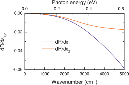
Figure 6: The ’sensitivity functions’ $(\partial R/\partial\epsilon_{1})(\omega)$, and $(\partial R/\partial\epsilon_{2})(\omega)$ in the near- and far-infrared, obtained for Bi2212 near optimal doping at $T_{c}$= 88 K as described in Appendix A2.

Appendix A2. Determination of $(\partial R/\partial\epsilon_{1,2})(\omega,T_{c})$

The application of the slope-difference analysis in the range where only $R(\omega)$ is measured requires the knowledge of ’sensitivity functions’ $(\partial R/\partial\epsilon_{1,2})(\omega)$, taken at $T_{c}$. We determine them from a Drude-Lorentz model, which fits well both $R(\omega)$ and the ellipsometrically measured $\epsilon_{1}(\omega)$ and $\epsilon_{2}(\omega)$ at higher frequencies. The accuracy in this case is superior to the usual KK transform of reflectivity, since the high-frequency ellipsometry data effectively ’anchor’ the phase of $R$ at low frequencies BozovicPRB90 ; KuzmenkoCM05 . The result is shown in Fig.6. Both $(\partial R/\partial\epsilon_{1})(\omega,T_{c})$ and $(\partial R/\partial\epsilon_{1})(\omega,T_{c})$ are rather structureless and vanishing, as $\omega$ goes to 0.

References

- (1) H. J. A. Molegraaf, C. Presura, D. van der Marel, P. H. Kes, and M. Li, Science 295, 2239 (2002).
- (2) A. F. Santander-Syro, R. P. S. M. Lobo, N. Bontemps, Z. Konstatinovic, Z. Z. Li, and H. Raffy, Europhys. Lett. 62, 568 (2003).
- (3) A. V. Boris, N. N. Kovaleva, O. V. Dolgov, T. Holden, C. T. Lin, B. Keimer, and C. Bernhard, Science 304, 708 (2004).
- (4) J. Schützmann, H. S. Somal, A. A. Tsvetkov, D. van der Marel, G. E. J. Koops, N. Koleshnikov, Z. F. Ren, J. H. Wang, E. Brück, and A. A. Menovsky, Phys. Rev. B 55, 11118 (1997).
- (5) K. A. Moler, J. R. Kirtley, D. G. Hinks, T. W. Li, and Ming Xu, Science 279, 1193 (1998).
- (6) A. A. Tsvetkov, D. van der Marel, K. A. Moler, J. R. Kirtley, J. L. de Boer, A. Meetsma, Z. F. Ren, N. Koleshnikov, D. Dulic, A. Damascelli, M. Grüninger, J. Schützmann, J. W. van der Eb, H. S. Somal, and J. H. Wang, Nature 395, 360 (1998).
- (7) J. R. Kirtley, K. A. Moler, G. Villard, and A. Maignan, Phys. Rev. Lett. 81, 2140 (1998).
- (8) M. B. Gaifullin, Yuji Matsuda, N. Chikumoto, J. Shimoyama, K. Kishio, and R. Yoshizaki, Phys. Rev. Lett. 83, 3928 (1999).
- (9) D. N. Basov, S. I. Woods, A. S. Katz, E. J. Singley, R. C. Dynes, M. Xu, D. G. Hinks, C. C. Homes, and M. Strongin, Science 283, 49 (1999).
- (10) A. V. Boris, D. Munzar, N. N. Kovaleva, B. Liang, C. T. Lin, A. Dubroka, A. V. Pimenov, T. Holden, B. Keimer, Y. -L. Mathis, and C. Bernhard, Phys. Rev. Lett. 89, 277001 (2002).
- (11) A. B. Kuzmenko, N. Tombros, H. J. A. Molegraaf, M. Grüninger, D. van der Marel, and S. Uchida, Phys. Rev. Lett. 91, 037004 (2003).
- (12) D. van der Marel, Optical signatures of electron correlations in the cuprates. Chapter in Strong interactions in low dimensions, edited by D. Baeriswyl and L. Degiorgi, in press, Kluwer (2004); cond-mat/0301506.
- (13) G. Deutscher, A. F. Santander-Syro, and N. Bontemps, cond-mat/0503073.
- (14) J. E. Hirsch, Physica C 201, 347 (1992).
- (15) P. W. Anderson, Science 268, 1154 (1995).
- (16) A. J. Leggett, Science 274, 587 (1996).
- (17) S. Chakravarty, Eur. Phys. J. B 5, 337 (1998).
- (18) S. Chakravarty, Hae-Young Kee, and E. Abrahams, Phys. Rev. Lett. 82, 2366 (1999).
- (19) D. Munzar, C. Bernhard, T. Holden, A. Golnik, J. Humlicek, and M. Cardona, Phys. Rev. B 64, 024523 (2001).
- (20) D. Munzar, T. Holden, and C. Bernhard, Phys. Rev. B 67, R020501 (2003).
- (21) M. R. Norman and C. Pépin, Phys. Rev. B 66, 100506 (2002).
- (22) D. van der Marel, H. J. A. Molegraaf, C. Presura, and I. Santoso, in Concepts in electron correlation, edited by A. Hewson and V. Zlatic, Kluwer (2003); cond-mat/0302169.
- (23) A. Knigavko, J. P. Carbotte, and F. Marsiglio, Phys. Rev. B 70, 224501 (2004).
- (24) A. Abanov and A. V. Chubukov, Phys. Rev. B 70, 100504 (2004).
- (25) L. Benfatto, S. G. Sharapov, and H. Beck, Europhys. J. B 39, 469 (2004).
- (26) P. W. Anderson, P. A. Lee, M. Randeria, T. M. Rice, N. Trivedi, and F. C. Zhang, J. Phys. Condens. Matter 16, R755 (2004).
- (27) J. E. Hirsch, Phys. Rev. B 69, 214515 (2004).
- (28) T. D. Stanescu, and P. Phillips, Phys. Rev. B 69, 245104 (2004).
- (29) T. A. Maier, M. Jarrell, A. Macridin, and C. Slezak, Phys. Rev. Lett. 92, 027005 (2004).
- (30) B. Farid, Philos. Mag. 84, 109 (2004).
- (31) M. Cardona, Modulation Spectroscopy, Academic, New York, (1969).
- (32) M. J. Holcomb, J. P. Collman, and W. A. Little, Phys. Rev. Lett. 73, 2360 (1994).
- (33) A. B. Kuzmenko, cond-mat/0503565.
- (34) The definition of being positive to indicate a decrease of below is somewhat confusing. In this work we use the opposite definition.
- (35) The KK relation was already a crucial argument in the analysis, presented in Ref.MolegraafScience02, .
- (36) M. Ortolani, P. Calvani, and S. Lupi, Phys. Rev. Lett. 94, 067002 (2005)
- (37) A. Toschi, M. Capone, M. Ortolani, P. Calvani, S. Lupi, and C. Castellani, cond-mat/0502528.
- (38) D. van der Marel, H. J. A. Molegraaf, J. Zaanen, Z. Nussinov, F. Carbone, A. Damascelli, H. Eisaki, M. Greven, P. H. Kes, and M. Li, Nature 425, 271 (2003).
- (39) A. E. Karakozov, E. G. Maksimov, and O. V. Dolgov, Solid State Commun. 124, 119 (2002).
- (40) M. Rübhausen, A. Gozar, M. V. Klein, P. Guptasarma, and D. G. Hinks, Phys. Rev. B, 63, 224514 (2001).
- (41) A. Junod, A. Erb, and C. Renner, Physica C 317, 333 (1999).
- (42) J. W. Loram, J. Luo, J. R. Cooper, W. Y. Liang and, J. L. Tallon, J. Phys. Chem. Solids 62, 59 (2001).
- (43) In Bi2212, one observes that the temperature dependent quantities such as the entropy, , do not have a real kink, but rather an inflection point at . Correspondingly the specific heat, , has a lambda-like maximum at instead of a sharp specific heat jump. Fitting the temperature dependence over some finite temperature range above and below with a second order polynomial, and taking the slope difference as we do, measures the slope change over the fluctuation region around . If the fluctuation region becomes too broad, it becomes increasingly difficult to separate the superconductivity induced effects from the normal state trends. For Bi2212 near optimal doping, which is the case which we consider here, the fluctuation region is sufficiently narrow (see Ref.CorsonNature99, ), allowing an unproblematic and meaningful kink-analysis.
- (44) I. Bozovic, Phys. Rev. B 42, 1969 (1990).
- (45) O. V. Dolgov, A. E. Karakozov, A. M. Mikhailovsky, B. J. Feenstra, and D. van der Marel, Physica C 229, 6360 (1994).
- (46) The only requirement for the KK-consistency of the dispersion model (8) is that all .
- (47) All data modeling was done, using an automated non-linear fitting routine, implemented in RefFIT software (http://optics.unige.ch/alexey/reffit.html).
- (48) H. J. A. Molegraaf, PhD thesis, Rijksuniversiteit Groningen (2005). Available on-line at http://irs.ub.rug.nl/ppn/271449179.
- (49) Shih-Fu Lee, D. C. Morgan, R. J. Ormeno, D. M. Broun, R. A. Doyle, and J. R. Waldram, Phys. Rev. Lett. 77, 735 (1996).
- (50) We note, that the symbol size of the curve , reported in Ref.BorisScience04, for Bi2212 (Fig. S6 A) does not exclude a slight downward kink at , in agreement with our data.
- (51) D. I. Khomskii and F. V. Kusmartsev, Phys. Rev. B 46, 14245 (1992).
- (52) J. Corson, R. Mallozzi, J. Orenstein, J. N. Eckstein, and I. Bozovic, Nature 398, 221 (1999).