Dynamical behavior across the Mott transition of two bands with different bandwidths

Abstract

We investigate the role of the bandwidth difference in the Mott metal-insulator transition of a two-band Hubbard model in the limit of infinite dimensions, by means of a Gutzwiller variational wave function as well as by dynamical mean-field theory. The variational calculation predicts a two-stage quenching of the charge degrees of freedom, in which the narrower band undergoes a Mott transition before the wider one, both in the presence and in the absence of a Hund’s exchange coupling. However, this scenario is not fully confirmed by the dynamical mean-field theory calculation, which shows that, although the quasiparticle residue of the narrower band is zero within our numerical accuracy, low-energy spectral weight still exists inside the Mott-Hubbard gap, concentrated into two peaks symmetric around the chemical potential. This spectral weight vanishes only when the wider band ceases to conduct too. Although our results are compatible with several scenarios, e.g., a narrow gap semiconductor or a semimetal, we argue that the most plausible one is that the two peaks coexist with a narrow resonance tied at the chemical potential, with a spectral weight below our numerical accuracy. This quasiparticle resonance is expected to vanish when the wider band undergoes the Mott transition.

I Introduction

Unlike in single-band models, the Mott metal-insulator transition (MIT) in multi-orbital strongly correlated systems generically involves other energy scales besides the short range Coulomb repulsion $U$ and the bare electron bandwidth. They include, for instance, the Coulomb exchange $J$ which produces the Hund’s rules, any crystal field or Jahn-Teller effect splitting the orbital degeneracy, and possibly bandwidth differences between the orbitals. There are many theoretical works making use of the so-called Dynamical Mean-Field Theory (DMFT) georges1996 which analyze the role of the exchange $J$, Bulla the crystal field splitting, Manini and the Jahn-Teller effect. Han ; Massimo All these analysis suggest that these perturbations, which have the common feature of splitting multiplets at fixed charge, are amplified near the MIT, leading for instance to an appreciable shift of the transition towards lower $U$’s Bulla or to the appearance of anomalous phases just before the MIT. Massimo This behavior is not surprising, since the more the electronic motion is slowed down, i.e., the longer is the time electrons stay localized around a site, the larger is the chance to get advantage of multiplet-splitting mechanisms.

On the contrary, the role of different bandwidths for nearly degenerate orbitals is less predictable, since the Coulomb charge repulsion only cares about the total number of electrons at a given site, while it is not concerned with the orbital they sit in. Recently, this issue has been addressed in a two-band Hubbard model by DMFT, yet leading to controversial results. Liebsch has suggested, on the basis of a DMFT calculation using quantum Monte Carlo as impurity solver, that both with $J=0$ and $J\not=0$ the two orbitals undergo a common MIT, whatever the difference between their bandwidths. liebsch2003 ; liebsch2004 This conclusion has been questioned by Koga and coworkers, koga2004 again by DMFT, using, however, exact diagonalization instead of quantum Monte Carlo. Their conclusion is that the MIT is unique only if $J=0$. On the contrary, when $J\not=0$, there is a first transition at which the orbital with smaller bandwidth becomes insulating, followed at larger values of the interaction by a second transition at which the other orbital ceases to conduct as well. This two-stage quenching of the charge degrees of freedom has been named Orbital-Selective Mott Transition (OSMT) by those authors. Although the coexistence of localized $f$-electrons and itinerant $d$-electrons is not unusual in rare-earth compounds, the conclusions of Ref. koga2004, are a bit surprising in the case of degenerate orbitals. Indeed, the Coulomb exchange-splitting, rather than favoring an OSMT, should naïvely oppose to it, since $J$ competes against the angular momentum quenching due to the different bandwidths.

In this work, we attempt to clarify this issue by means of a variational analysis based on Gutzwiller wave functions, by standard DMFT calculations as well as by an approximate DMFT projective technique. The paper is organized as follows. In Section II, we introduce the two-band model and discuss general properties. In Section III, we apply a variational technique based on Gutzwiller-type trial wave functions to analyze the ground state of the Hamiltonian. A full DMFT analysis is presented in Section IV. As a guide to interpret the DMFT spectral functions, in Section V, we show the density of state obtained by Wilson Numerical Renormalization Group NRG of the Anderson impurity model onto which the lattice model maps within DMFT. In Section VI, we present an approximate DMFT solution obtained by projecting out self-consistently high-energy degrees of freedom, which allow a better low-energy description. Conclusions are drawn in Section VII.

II The model

We consider a two-band Hubbard model at half-filling described by the Hamiltonian

$$\mathcal{H} = -\sum_{\langle i,j\rangle,\sigma}\,\sum_{a=1}^{2}\,t_{a}\,f^{\dagger}_{i,a\sigma}f^{\phantom{\dagger}}_{j,a\sigma}+H.c.$$ (1)

$$+\frac{U}{2}\sum_{i}\,\left(n_{i}-2\right)^{2}+\mathcal{H}_{\rm exch},$$

where $f^{\dagger}_{i,a\sigma}$ creates an electron at site $i$ in orbital $a=1,2$ with spin $\sigma$, $n_{i\,a}=\sum_{\sigma}\,f^{\dagger}_{i,a\sigma}f^{\phantom{\dagger}}_{i,a\sigma}$ is the occupation number at site $i$ in orbital $a$, and $n_{i}=n_{i\,1}+n_{i\,2}$ is the total occupation number. The explicit expression of the Coulomb exchange $\mathcal{H}_{\rm exch}$ is

$$\mathcal{H}_{\rm exch} = \frac{J}{2}\sum_{i}\,\left(n_{i\,1}-n_{i\,2}\right)^{2}$$

$$+\frac{J}{2}\sum_{i}\,\sum_{\sigma,\sigma^{\prime}}\,f^{\dagger}_{i,1\sigma}f^{\dagger}_{i,1\sigma^{\prime}}f^{\phantom{\dagger}}_{i,2\sigma^{\prime}}f^{\phantom{\dagger}}_{i,2\sigma}+H.c.$$

$$+\frac{J}{4}\sum_{\sigma,\sigma^{\prime}}f^{\dagger}_{i,1\sigma}f^{\phantom{\dagger}}_{i,2\sigma}f^{\dagger}_{i,2\sigma^{\prime}}f^{\phantom{\dagger}}_{i,1\sigma^{\prime}}+H.c.$$

$$\equiv 2J\,\sum_{i}\,\left(T_{i\,x}^{2}+T_{i\,z}^{2}\right),$$ (3)

where

$$T_{i\,\alpha}=\frac{1}{2}\sum_{a,b}\,\sum_{\sigma}\,f^{\dagger}_{i,a\sigma}\,\tau^{\alpha}_{ab}\,f^{\phantom{\dagger}}_{i,b\sigma}$$ (4)

are pseudo-spin-1/2 operators, with $\tau^{\alpha}$ the Pauli matrices, $\alpha=x,y,z$. In what follows, we always take $0<t_{2}\leq t_{1}$. Let us start by discussing some general properties of this Hamiltonian.

If $U\gg t_{1}$, the model describes a Mott insulator in which two electrons localize on each site. For $J>0$, the atomic two-electron ground state is the spin triplet, followed at energy $2J$ by the two degenerate singlets (we drop the site index):

$$\sqrt{\frac{1}{2}}\left(f^{\dagger}_{1\uparrow}f^{\dagger}_{2\downarrow}+f^{\dagger}_{2\uparrow}f^{\dagger}_{1\downarrow}\right)\,|0\rangle,\;\;\sqrt{\frac{1}{2}}\left(f^{\dagger}_{1\uparrow}f^{\dagger}_{1\downarrow}-f^{\dagger}_{2\uparrow}f^{\dagger}_{2\downarrow}\right)\,|0\rangle,$$

and finally at energy $4J$ by the singlet:

$$\sqrt{\frac{1}{2}}\left(f^{\dagger}_{1\uparrow}f^{\dagger}_{1\downarrow}+f^{\dagger}_{2\uparrow}f^{\dagger}_{2\downarrow}\right)\,|0\rangle.$$

Hence, the Mott insulator for very large $U$, specifically $t_{1}^{2}/U\ll J$, is effectively a spin-1 Heisenberg model where, at any site, each orbital is occupied by one electron, the two electrons being bound into a spin-triplet configuration. Within the OSMT scenario, below some critical repulsion, defined in the following as $U_{1}$, electrons in orbital 1 start moving, while one electron per site remains localized in orbital 2. Only below a lower $U_{2}<U_{1}$, electrons in orbital 2 delocalize too. In this particular example with a half-filled shell, the Coulomb exchange does not conflict with the OSMT, since $\mathcal{H}_{\rm exch}$ favors single occupancy of each orbital. Yet, one may wonder about the role of the pair-hopping term (II) which can transfer electrons from the delocalized orbital to the localized one.

III Gutzwiller variational technique

Let us start by a variational analysis of the ground state of the Hamiltonian (1). In particular, we are going to use the Gutzwiller variational approach, which is one of the simplest way to include electronic correlations into a many-body wave function. In what follows, we briefly introduce this variational technique for a generic multi-orbital model, and later we apply it to our specific example.

Let us consider in general a $k$-orbital Hamiltonian that contains, besides the hopping term

$$\mathcal{H}_{0}=-\sum_{\langle i,j\rangle,\sigma}\,\sum_{a=1}^{k}\,t_{a}\,f^{\dagger}_{i,a\sigma}f^{\phantom{\dagger}}_{j,a\sigma}+H.c.,$$ (5)

an on-site interaction of the general form

$$\mathcal{H}_{\rm int}=\sum_{i}\,\sum_{n,\Gamma}\,U(n,\Gamma)\,\mathcal{P}_{i}(n,\Gamma),$$ (6)

where $\mathcal{P}_{i}(n,\Gamma)=|i;n,\Gamma\rangle\langle i;n,\Gamma|$ is the projector operator onto the site-$i$ configuration $\Gamma$ with $n$ electrons. If $|\Psi_{0}\rangle$ is the Fermi-sea Slater determinant of the non-interacting Hamiltonian, the Gutzwiller wave function $|\Psi\rangle$ is defined through

$$|\Psi\rangle=\mathcal{P}_{G}\,|\Psi_{0}\rangle=\prod_{i}\mathcal{P}_{i\,G}\,|\Psi_{0}\rangle,$$ (7)

where the operator $\mathcal{P}_{i\,G}$ acts on site $i$ and is given by

$$\mathcal{P}_{i\,G}=\sum_{n,\Gamma}\,\lambda_{n\Gamma}\,\mathcal{P}_{i}(n,\Gamma).$$ (8)

The $\lambda_{n\Gamma}$’s in (8) are variational parameters which modify the weights of the on-site configurations $|i;n,\Gamma\rangle$ in accordance with the interaction (6). Following Ref. Gebhard, , we assume, without loss of generality, Attaccalite that

$$\langle\Psi_{0}|\mathcal{P}_{i\,G}^{2}|\Psi_{0}\rangle = \langle\Psi_{0}|\Psi_{0}\rangle=1,$$ (9)

$$\langle\Psi_{0}|\,\mathcal{P}_{i\,G}^{2}\,f^{\dagger}_{i,a\sigma}f^{\phantom{\dagger}}_{i,b\sigma^{\prime}}\,|\Psi_{0}\rangle = \langle\Psi_{0}|f^{\dagger}_{i,a\sigma}f^{\phantom{\dagger}}_{i,b\sigma^{\prime}}|\Psi_{0}\rangle$$ (10)

$$= \frac{N}{2k}\,\delta_{ab}\,\delta_{\sigma\sigma^{\prime}},$$

where $N$ is the average occupation per site within the Fermi sea, in which all orbitals are equally occupied by our choice of the hopping term (5). These two conditions allow an analytic evaluation of any average value over the correlated wave function in infinite dimensions. Gebhard In particular, one can show that (9) is satisfied by

$$\lambda_{n\Gamma}^{2}=\frac{P(n,\Gamma)}{P^{(0)}(n,\Gamma)},$$ (11)

where

$$P(n,\Gamma)=\langle\Psi|{\cal{P}}_{i}(n,\Gamma)|\Psi\rangle,$$ (12)

is the correlated probability distribution of the on-site configuration $\Gamma$ with $n$ electrons and

$$P^{(0)}(n,\Gamma)=\langle\Psi_{0}|{\cal{P}}_{i}(n,\Gamma)|\Psi_{0}\rangle,$$ (13)

is the uncorrelated one. Therefore, rather than using the variational parameters $\lambda_{n\Gamma}$’s, one can directly work with the correlated probability distribution $P(n,\Gamma)$ which satisfies

$$\sum_{n,\Gamma}\,P(n,\Gamma)=1,\;\;\sum_{n,\Gamma}\,n\,P(n,\Gamma)=N.$$

By the above definitions, one can demonstrate Gebhard that the average value of the hopping in infinite dimensions reduces to

$$\langle\Psi|f^{\dagger}_{i,a\sigma}f^{\phantom{\dagger}}_{j,a\sigma}|\Psi\rangle = \langle\Psi_{0}|\mathcal{P}_{i\,G}\,f^{\dagger}_{i,a\sigma}\,\mathcal{P}_{i\,G}\,\mathcal{P}_{j\,G}\,f^{\phantom{\dagger}}_{j,a\sigma}\,\mathcal{P}_{j\,G}|\Psi_{0}\rangle$$ (14)

$$= Z_{a}\,\langle\Psi_{0}|f^{\dagger}_{i,a\sigma}f^{\phantom{\dagger}}_{j,a\sigma}|\Psi_{0}\rangle,$$

where the reduction factor $Z_{a}$ can be evaluated through

$$\sqrt{Z_{a}}=\frac{2k}{N}\langle\Psi_{0}|\mathcal{P}_{i\,G}\,f^{\dagger}_{i,\alpha\sigma}\,\mathcal{P}_{i\,G}\,f^{\phantom{\dagger}}_{i,\alpha\sigma}|\Psi_{0}\rangle.$$ (15)

In addition, the average value of the on-site interaction is found to be

$$\langle\Psi|\mathcal{H}_{\rm int}|\Psi\rangle=\sum_{i}\,\sum_{n,\Gamma}\,U(n,\Gamma)\,P(n,\Gamma).$$ (16)

III.1 Results for $J=0$

Let us apply this technique to our model (1), starting with the simpler case where $J=0$. We define as $P(0)$ and $P(4)$ the correlated probabilities of a site occupied by zero and four electrons, respectively. $P(1,+)$ and $P(1,-)$ are instead the probabilities of a singly-occupied site with one electron in orbital 2 and 1, respectively. Analogously, $P(3,+)$ and $P(3,-)$ are the probabilities of a site occupied by three electrons, with one hole in orbital 1 or 2, respectively. Finally, concerning doubly occupied sites, $P(2,1)$ is the probability of the spin-triplet configuration, $P(2,0)$ of the inter-orbital spin-singlet, $P(2,+)$ and $P(2,-)$ of the spin singlets with two electrons in orbital 2 and 1, respectively. By particle-hole symmetry, we have that

$$P(0) = P(4),$$

$$P(1,+) = P(3,-),$$

$$P(1,-) = P(3,+),$$

$$P(2,+) = P(2,-).$$

After some simple, but lengthy algebra, we find that the hopping energy reduction factors are

$$\sqrt{Z_{1}} = 2\,\sqrt{2}\,\sqrt{P(0)P(1,-)}+\sqrt{2}\,\sqrt{P(1,-)P(2,-)}$$

$$+\sqrt{2}\,\sqrt{P(1,-)P(2,+)}+\sqrt{2}\,\sqrt{P(1,+)P(2,0)}$$

$$+\sqrt{6}\,\sqrt{P(1,+)P(2,1)},$$

$$\sqrt{Z_{2}} = 2\,\sqrt{2}\,\sqrt{P(0)P(1,+)}+\sqrt{2}\,\sqrt{P(1,+)P(2,+)}$$

$$+\sqrt{2}\,\sqrt{P(1,+)P(2,-)}+\sqrt{2}\,\sqrt{P(1,-)P(2,0)}$$

$$+\sqrt{6}\,\sqrt{P(1,-)P(2,1)}.$$

Since $J=0$, the two-electron configurations with one electron in each orbital are equally probable, namely $P(2,1)=3P(2,0)$. Therefore, one can use the following parametrization

$$P(1,+) = P(1)\,\cos^{2}\phi,$$

$$P(1,-) = P(1)\,\sin^{2}\phi,$$

$$P(2,1) = P(2)\,\frac{3}{4}\,\cos^{2}\theta,$$

$$P(2,0) = P(2)\,\frac{1}{4}\,\cos^{2}\theta,$$

$$P(2,+) = P(2,-)=P(2)\,\frac{1}{2}\,\sin^{2}\theta.$$

The normalization condition now reads

$$2\,P(0)+2\,P(1)+P(2)=1,$$ (17)

and the $Z$-reduction factors can be written as

$$\sqrt{Z_{1}} = 2\,\sqrt{2}\,\sin\phi\,\sqrt{P(0)P(1)}$$

$$+\sqrt{P(1)P(2)}\,\left[2\,\sin\phi\,\sin\theta+\sqrt{8}\,\cos\phi\,\cos\theta\right],$$

$$\sqrt{Z_{2}} = 2\,\sqrt{2}\,\cos\phi\,\sqrt{P(0)P(1)}$$

$$+\sqrt{P(1)P(2)}\,\left[2\,\cos\phi\,\sin\theta+\sqrt{8}\,\sin\phi\,\cos\theta\right].$$

If we define

$$T = \frac{1}{V}\langle\Psi_{0}|\sum_{\langle i,j\rangle,\sigma}\,f^{\dagger}_{i,1\sigma}f^{\phantom{\dagger}}_{j,1\sigma}+H.c.|\Psi_{0}\rangle$$

$$= \frac{1}{V}\langle\Psi_{0}|\sum_{\langle i,j\rangle,\sigma}\,f^{\dagger}_{i,2\sigma}f^{\phantom{\dagger}}_{j,2\sigma}+H.c.|\Psi_{0}\rangle,$$

the average value per site of the hopping operator in the Fermi sea, then the variational energy of the Gutzwiller wave function in infinite dimensions is

$$E=-t_{1}\,T\,Z_{1}-t_{2}\,T\,Z_{2}+U\,P(1)+4\,U\,P(0).$$ (18)

Here, the $Z_{i}$’s are functionals of the probability distribution $P(n)$, $n=0,1,2$, with the normalization (17), as well as of the two angles $\phi,\theta\in[0,\pi/2]$.

One can proceed analytically a bit further. It is known that near a Mott transition and within the Gutzwiller wave function approach, one can safely neglect $P(0)=P(4)$. Attaccalite Within this approximation, $P(2)=1-2\,P(1)$ and

$$\sqrt{Z_{1}} = \sqrt{P(1)P(2)}\,\left[2\,\sin\phi\,\sin\theta+\sqrt{8}\,\cos\phi\,\cos\theta\right],$$

$$\sqrt{Z_{2}} = \sqrt{P(1)P(2)}\,\left[2\,\cos\phi\,\sin\theta+\sqrt{8}\,\sin\phi\,\cos\theta\right].$$

We denote $P(1)=d/2$, hence $P(2)=1-d$, so that the variational energy (18) becomes

$$E=-T\,\frac{d\,(1-d)}{2}\,f(\phi,\theta)+\frac{U}{2}\,d$$

where

$$f(\phi,\theta) = t_{1}\,\left[2\,\sin\phi\,\sin\theta+\sqrt{8}\,\cos\phi\,\cos\theta\right]^{2}$$

$$+t_{2}\,\left[2\,\cos\phi\,\sin\theta+\sqrt{8}\,\sin\phi\,\cos\theta\right]^{2}.$$

The optimal value for $d$ is

$$d_{*}=\frac{T\,f(\phi,\theta)-U}{2\,T\,f(\phi,\theta)},$$

and the variational energy becomes:

$$E[\phi,\theta]=-\frac{\left[T\,f(\phi,\theta)-U\right]^{2}}{8\,T\,f(\phi,\theta)}.$$

At given $\phi$ and $\theta$, the Mott transition at which both orbitals localize occurs when $d_{*}=0$, namely when

$$U_{c}(\phi,\theta)=T\,f(\phi,\theta).$$

The most stable solution is the one which maximizes $f$. An OSMT corresponds to a situation in which the Mott transition occurs with orbital 2 being already strictly singly-occupied, namely with $\phi=\theta=0$. This solution is an extremum of $f$. Yet, one has to check whether it is also a maximum. We find that this is indeed the case whenever

$$t_{2}\leq\frac{1}{5}\,t_{1}.$$ (19)

Therefore, within the Gutzwiller variational technique, an OSMT can occur even in the absence of Coulomb exchange, provided (19) is satisfied.

We optimized (18) numerically, considering an infinite coordination Bethe lattice at half-filling. The free density of state is given by

$$\rho_{a}(\epsilon)=\frac{\sqrt{4t^{2}_{a}-\epsilon^{2}}}{2\pi t^{2}_{a}},$$ (20)

and, in this case, $T=8/(3\pi)$. The half-bandwidth of each band is $D_{a}=2t_{a}$, and our unit of energy is $D_{1}$. The reduction factors $Z_{1}$ and $Z_{2}$ are shown in Fig. 1, for different ratios $D_{2}/D_{1}$. The results indeed confirm the analytical calculation (19), displaying two distinct transitions when $D_{2}/D_{1}<0.20$.

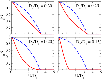
Figure 1: Reduction factors $Z_{a}$ for the wide band (dashed line) and for the narrow band (continuous line) obtained with the Gutzwiller wave function for different ratios of the bandwidth $D_{2}/D_{1}$ and $J=0$.

III.2 Results for $J\not=0$

Let us now move to the more complicated case of $J\not=0$. The Hund’s rule coupling acts only within the two-electron configurations and can be written as

$$\mathcal{H}_{J} = \sum_{i}\,-\frac{4}{3}J\,|i;2,1\rangle\langle i;2,1|+\frac{2}{3}J\,|i;2,0\rangle\langle i;2,0|$$ (21)

$$+\frac{5}{3}J\,\left(\,|i;2,+\rangle\langle i;2,+|+|i;2,-\rangle\langle i;2,-|\,\right)$$

$$+J\,\left(\,|i;2,+\rangle\langle i;2,-|+|i;2,-\rangle\langle i;2,+|\,\right),$$

using the previous notation for the two-electron configurations. Since it is not diagonal in the representation which we have used so far, we are forced to generalize the Gutzwiller correlator (8) into Attaccalite

$$\mathcal{P}_{i\,G}\rightarrow\mathcal{P}_{i\,G}+\lambda_{2\,\perp}\left(|2,+\rangle\langle 2,-|+|2,-\rangle\langle 2,+|\right).$$ (22)

Consequently,

$$P(2,+) = \lambda_{2\,+}^{2}\,P^{(0)}(2,+)+\lambda_{2\,\perp}^{2}\,P^{(0)}(2,-),$$

$$P(2,-) = \lambda_{2\,-}^{2}\,P^{(0)}(2,-)+\lambda_{2\,\perp}^{2}\,P^{(0)}(2,+).$$

Since by particle-hole symmetry $P(2,+)=P(2,-)$, as well as $P^{(0)}(2,+)=P^{(0)}(2,-)$, then $\lambda_{2\,+}=\lambda_{2\,-}\equiv\lambda_{2\,\pm}$ and hence

$$\lambda_{2,\pm}^{2}+\lambda_{2,\perp}^{2}=\frac{P(2,+)}{P^{(0)}(2,+)}.$$

In addition, the following matrix element is non zero

$$A(2,\pm)\equiv\langle\Psi|\,2,+\rangle\langle 2,-\,|\Psi\rangle=2\,\lambda_{2,\perp}\,\lambda_{2,\pm}\,P^{(0)}(2,+),$$ (23)

so that

$$\lambda_{2,\pm} = \frac{1}{2\sqrt{P^{(0)}(2,+)}}\left[\sqrt{P(2,+)+A(2,\pm)}\right.$$

$$\left.+\sqrt{P(2,+)-A(2,\pm)}\right],$$

$$\lambda_{2,\perp} = \frac{1}{2\sqrt{P^{(0)}(2,+)}}\left[\sqrt{P(2,+)+A(2,\pm)}\right.$$

$$\left.-\sqrt{P(2,+)-A(2,\pm)}\right].$$

We notice that $|A(2,\pm)|\leq P(2,+)$. The hopping reduction factors are consequently modified into

$$\sqrt{Z_{1}} = 2\sqrt{2}\,\sqrt{P(0)P(1,-)}$$

$$+\sqrt{2}\,\sqrt{P(1,-)}\left[\sqrt{P(2,+)+A(2,\pm)}\right.$$

$$\left.+\sqrt{P(2,+)-A(2,\pm)}\right]$$

$$+\sqrt{2}\,\sqrt{P(1,+)P(2,0)}+\sqrt{6}\,\sqrt{P(1,+)P(2,1)},$$

$$\sqrt{Z_{2}} = 2\sqrt{2}\,\sqrt{P(0)P(1,+)}$$

$$+\sqrt{2}\,\sqrt{P(1,+)}\left[\sqrt{P(2,+)+A(2,\pm)}\right.$$

$$\left.+\sqrt{P(2,+)-A(2,\pm)}\right]$$

$$+\sqrt{2}\,\sqrt{P(1,-)P(2,0)}+\sqrt{6}\,\sqrt{P(1,-)P(2,1)}.$$

The average value of the Hund’s coupling is

$$E_{J} = -\frac{4}{3}\,J\,P(2,1)+\frac{8}{3}\,J\,\left[P(2,+)+A(2,\pm)\right]$$ (24)

$$+\frac{2}{3}\,J\,\left[P(2,0)+P(2,+)-A(2,\pm)\right],$$

and that of the Hubbard repulsion

$$E_{U}=U\,\left[P(1,+)+P(1,-)\right]+4\,U\,P(0),$$ (25)

thus, the variational energy to be minimized is

$$E=-t_{1}\,T\,Z_{1}-t_{2}\,T\,Z_{2}+E_{J}+E_{U}.$$ (26)

By the numerical minimization of the variational energy, we find that the critical ratio $D_{2}/D_{1}$ for an OSMT increases when $J\not=0$ from the value 0.2 found for $J=0$. In Fig. 2, we show $Z_{1}$ and $Z_{2}$ as obtained by numerical minimization of (26), for two ratios of $D_{2}/D_{1}$ and $J/U=0.10$. Additional calculations allowed to draw the phase diagram within the Gutzwiller variational approach, see Fig. 3. As is apparent from the inset, the introduction of the Hund’s coupling increases the value of the critical ratio $D_{2}/D_{1}$. We also notice that the Mott transition at which both bands localize becomes first order in the presence of $J$, which, however, might be a pathology of the Gutzwiller wave function. Attaccalite

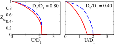
Figure 2: Reduction factors $Z_{a}$ for the wide band (dashed line) and the narrow band (continuous line) obtained with the Gutzwiller wave function for different ratios of the bandwidth $D_{2}/D_{1}$ and $J/U=0.10$.

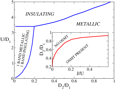
Figure 3: Phase diagram obtained within the Gutzwiller approximation in the absence of the Hund’s coupling. Inset: the critical ratio $D_{2}/D_{1}$ below which an OSMT is observed as a function of $J/U$.

In conclusion, we find that the Gutzwiller variational technique predicts an OSMT both for $J=0$ and $J\not=0$, provided $D_{1}/D_{2}$ is smaller than a critical value which increases with $J$.

IV Dynamical Mean-Field Theory

To have further insights on the quality of the Gutzwiller wave function in infinite dimensions, we have performed an extensive DMFT calculation for the same Hamiltonian. DMFT is a non-perturbative approach that neglects spatial correlations but retains fully time correlations and becomes exact for infinite-coordination lattices. In this limit, the lattice problem (1) can be mapped onto an Anderson impurity model supplemented by a self-consistency condition. For simplicity, we consider an infinite coordination Bethe lattice, as in the Gutzwiller variational approach, with a bare density of states given by (20). Again, $D_{a}=2t_{a}$ is the half-bandwidth of band $a$. The Anderson impurity model onto which the lattice model maps within DMFT is

$$\mathcal{H}_{\mathrm{AM}} = \sum_{k,a,\sigma}\epsilon_{ka}c^{\dagger}_{ka\sigma}c^{\phantom{\dagger}}_{ka\sigma}+\sum_{k,a,\sigma}V_{ka}\left(f^{\dagger}_{a\sigma}c^{\phantom{\dagger}}_{ka\sigma}+H.c.\right)$$ (27)

$$+ \frac{U}{2}(n_{f}-2)^{2}+2J\left(T_{x}^{2}+T_{z}^{2}\right),$$

where $T_{\alpha}$, $\alpha=x,y,z$, are the pseudo-spin operators (4) for the impurity. The self-consistency condition relates the impurity Green’s function for orbital $a$, $G_{a}$, to the parameters $\epsilon_{ka}$ and $V_{ka}$ through

$$t_{a}^{2}G_{a}(i\omega_{n})=\sum_{k}\frac{V_{ka}^{2}}{i\omega_{n}-\epsilon_{ka}}.$$ (28)

We solve the Anderson impurity model using an exact diagonalization method caffarel1994 at zero temperature. The continuous conduction-electron bath is modeled by a finite number of parameters $\epsilon_{ka}$ and $V_{ka}$ ($k=1,\ldots,n_{s}-1$). In our calculations, we considered $n_{s}=6$ and $4$ (not shown). The self-consistency (28) is implemented through a fitting procedure along the imaginary axis. To this end, we discretize the axis into Matsubara frequencies $i\omega_{n}=(2n+1)\pi/\beta$, where $\beta$ is a fictitious temperature that we have set to $\beta=500$. Moreover, the smallest frequency $\omega_{min}$ has been determined by the smallest pole in the continued fraction expansion of the Green’s function. moeller1995 Note that this procedure sometimes leads to different minimum cutoff frequencies for the two orbitals. In the following, we will work in units of $D_{1}$.

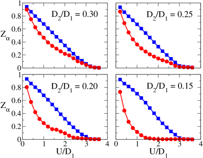
Figure 4: Quasiparticle residues $Z_{a}$ for the wide band (squares) and for the narrow band (circles) obtained by the DMFT calculation for different ratios of the bandwidth $D_{2}/D_{1}$ and $J=0$.

First, we treat the case in which there is no Hund’s coupling (i.e., $J=0$). The metallic or insulating nature of each band is characterized by its quasiparticle residue $Z_{a}^{-1}=1-\left(\partial\mathcal{I}m\Sigma_{a}(i\omega)/\partial i\omega\right)\lvert_{\omega\rightarrow 0}$. In Fig. 4, we show $Z_{a}$ as a function of the Coulomb repulsion $U$ for different bandwidth ratios $D_{2}/D_{1}$. When the ratio of the bandwidth $D_{2}/D_{1}\geq 0.20$, the quasiparticle weights decrease as the Coulomb interaction gets bigger. Even though there is a stronger initial reduction for the narrow band, the weights eventually vanish for the same critical value of $U_{c}/D_{1}\simeq 3.6$. The situation changes when we further decrease the bandwidth ratio (i.e., $D_{2}/D_{1}=0.15$). In this case, we find that the weights of the bands vanish for different values of $U$, in agreement with the results of the Gutzwiller wave function. Moreover, the critical ratio $D_{2}/D_{1}=0.20$ that we found earlier seems consistent with the DMFT calculation.

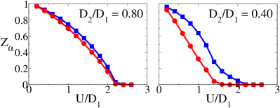
Figure 5: Quasiparticle residues $Z_{a}$ for the wide band (squares) and the narrow band (circles) obtained by the DMFT calculation for different ratios of the bandwidth $D_{2}/D_{1}$ and $J/U=0.10$.

Let us turn now to the model in the presence of a finite Hund’s coupling, $J/U=0.10$, and perform the same calculations for the following ratios of the bandwidths: $D_{2}/D_{1}=0.80$ and $0.40$. The results are shown in Fig. 5. We still find evidences for an OSMT, this time, however, below a larger ratio of the bandwidths. Further calculations show that the critical ratio of the bandwidth for $J/U=0.10$ is $D_{2}/D_{1}\sim 0.60$.

If we were to confine our analysis to the behavior of the quasiparticle residues $Z_{a}$’s, we should conclude that, both in the absence and in the presence of a Hund’s coupling, the OSMT scenario does occur for sufficiently small ratio of the bandwidth, in qualitative and also quantitative agreement with the variational results of the Gutzwiller wave function. The only difference may lie in the order of the transition. Even if it is difficult to settle precisely the order of the transition within DMFT, our results seem to point towards a second-order phase transition at the MIT $U_{1}$ with finite $J$, contrary to the first-order transition predicted by the Gutzwiller wave function.

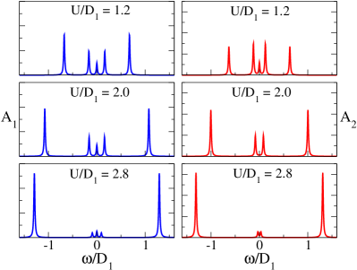
Figure 6: Density of states for the wide band (left panels) and the narrow band (right panels) as obtained by DMFT for different values of the Coulomb interaction. The ratio of the bandwidth is $D_{2}/D_{1}=0.15$ and $J=0$.

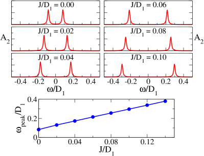
Figure 7: Upper panels: low-energy part of the density of states of the narrow band as obtained by DMFT for different values of $J/D_{1}$. The ratio of the bandwidths is $D_{2}/D_{1}=0.15$, and the Coulomb repulsion is set to $U/D_{1}=2$. Lower panel: position of the low-energy peaks as a function of $J/D_{1}$.

A deeper insight into the above scenario can be gained by analyzing the spectral properties of the more correlated band, and not just its quasiparticle residue. Indeed, such an inspection leads to a less clear-cut picture, revealing features which are not captured by the Gutzwiller wave function. In Fig. 6, we show the density of states (DOS) of both orbitals for various Hubbard $U$’s and $D_{2}/D_{1}=0.15$. We notice that, although the DOS of the narrow band right at the chemical potential becomes zero within our numerical accuracy above $U_{2}$, there is still low-energy spectral weight inside the Mott-Hubbard gap. Due to our discretization procedure, this weight is concentrated in two peaks located symmetrically with respect to the chemical potential. These peaks are also present at $J=0$, and move linearly away from the chemical potential when $J\not=0$, roughly as $2J$, see Fig. 7. Their total spectral weight scales approximately like the quasiparticle residue of the wider band, $Z_{1}$, both vanishing at the second MIT, $U_{1}$. In addition, if $J=0$, the distance between the peaks also scales like $Z_{1}$, see Fig. 6. If we, reasonably, assume that these two peaks mimic two resonances, one below and the other above the chemical potential, it becomes much less obvious what might be the actual value of the DOS right at the chemical potential if we were not constrained to a small number of levels. Moreover, even if the DOS were strictly zero at the chemical potential, still we should determine whether band 2 behaves like a small-gap semiconductor or a semimetal for $U_{2}\leq U\leq U_{1}$. In other words, the energy discretization inherent in the exact diagonalization technique might play a more critical role in our case than in the simplest single-band Hubbard model.

Therefore, although the numerical evidences we have presented so far point in favor of the existence of an OSMT with zero or finite $J$ below a critical bandwidth ratio, there are several aspects which still need to be clarified. We will consider a deeper investigation of such aspects in the following sections.

V Single impurity spectral properties

The first issue we want to address concerns the origin of the two peaks in the orbital 2 spectral function inside the Mott-Hubbard gap. Although the self-consistency condition (28) of the effective Anderson impurity model (27) plays a very crucial role, for instance it determines a critical value of $U$ above which the Kondo effect does not take place anymore, yet useful information can be obtained by studying (27) without imposing (28), which is what we are going to do in this section by means of the Wilson Numerical Renormalization Group (NRG). NRG

The Anderson impurity model (27) is controlled by several energy scales, the Hubbard $U$, the Hund’s coupling $J$ and the so-called hybridization widths

$$\Gamma_{a}=\sum_{k}\,V_{ka}^{2}\,\delta\left(\epsilon_{ka}\right).$$

For simplicity, we will assume that the two conduction baths are degenerate with half-bandwidth $D$, which will be our unit of energy. In Fig. 8, we show the impurity spectral function of the orbital 2, $A_{2}(\omega)$, as obtained by NRG for $J=0$, $U=2D$, $\Gamma_{1}=D/(2\pi)$, and for several values of $\Gamma_{2}/\Gamma_{1}<1$. Since we do not impose any self-consistency, the DOS for any $\Gamma_{2}\not=0$ shows a Kondo resonance at the chemical potential, which narrows as $\Gamma_{2}$ decreases. In addition, there are two more peaks which move slightly away from the chemical potential as $\Gamma_{2}$ is reduced. These peaks actually resemble those we find in the DMFT calculation. Indeed, they move linearly as we switch on $J$, see Fig. 9, just like we observe within DMFT.

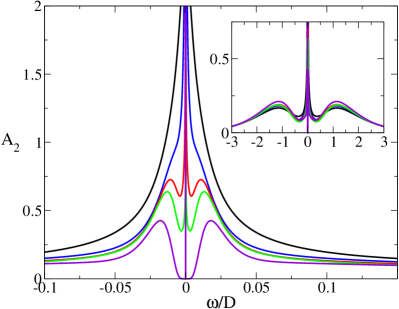
Figure 8: Spectral function $A_{2}(\omega)$ of the narrow band for $J=0$, $U/D=2$, $\Gamma_{1}=D/2\pi$, and $\Gamma_{2}/\Gamma_{1}=\frac{1}{2},\frac{1}{4},\frac{1}{6},\frac{1}{8},0$ (from top to bottom). Inset: the same spectral function on a wider scale.

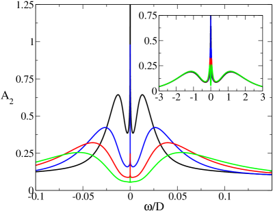
Figure 9: Spectral function $A_{2}(\omega)$ of the narrow band for $J/D=0,0.004,0.008,0.012$ (from top to bottom), $U/D=2$, $\Gamma_{1}=D/2\pi$, and $\Gamma_{2}/\Gamma_{1}=1/8$. Inset: the same spectral function on a wider scale.

The origin of these peaks is easy to identify when $\Gamma_{2}=0$. When the orbital 2 is not hybridized with its bath, its occupation number $n_{2}$ is a conserved quantity. The ground state is expected to belong to the subspace with $n_{2}=1$, because, in this case, $\langle n_{1}\rangle=1$ and the Kondo-screening energy gain is maximum. This state is twofold degenerate reflecting the free spin-1/2 of the electron localized in orbital 2. The energy gap to the lowest energy states for $n_{2}=0,2$, $\langle n_{1}\rangle=2,0$, respectively, is therefore of the order of the Kondo temperature of orbital 1, $T_{K\,1}$. The impurity orbital-2 DOS is analogous to the core-hole spectral function in X-ray absorption, so it should start above a finite threshold proportional to $T_{K\,1}$. In other words, the DOS has a small but finite gap of order $T_{K\,1}$, similar to what we observe within DMFT.

However, as soon as $\Gamma_{2}$ is non zero, this gap is filled and, in addition, a Kondo-resonance appears. Even if we move the peaks away from the chemical potential by increasing $J$, see Fig. 9, the region between them and the narrow (practically invisible in the figure) Kondo-resonance is still covered by spectral weight. In the light of this dynamical behavior, it is not at all obvious what the self-consistency requirement (28) may lead to when band-1 is still conducting. In other words, either a true narrow gap, as if $\Gamma_{2}=0$, or a pseudo-gap with a power-law vanishing DOS, or two-peaks plus the narrow resonance are equally compatible with the self-consistency condition. However, the event in which most of the spectral weight is concentrated in the two symmetric peaks, leaving only negligible weight within the narrow resonance, is extremely hard to identify with a limited number of levels. As an attempt to discriminate among the aforementioned possible scenarios, in the following section, we implement a projective self-consistency technique which allows a more detailed low-energy description within DMFT.

VI Projective Self-Consistent Technique

A remarkable feature uncovered by DMFT nearby a MIT is the clear separation of energy scales between well preformed high-energy Hubbard bands and lingering low-energy itinerant quasiparticles. It has been shown, moeller1995 that this partition of energy scales allows to reformulate the problem into a new one, in which the high-energy part is projected out. Essentially, the original Anderson impurity model, which involves both high-energy side-bands and low-energy quasiparticles, is reduced to a Kondo-like model which can be attacked more easily by a numerical procedure. In this section, we apply a projective technique to our model, which is similar to Ref. moeller1995, , with the only difference that the resulting effective problem is still an Anderson impurity model with rescaled parameters.

As we showed, the occurrence of an OSMT does not seem to require a finite exchange but rather a sufficiently small bandwidth ratio. Therefore, we prefer to present the projective technique in the simpler case where $J=0$. Following Ref. moeller1995, , we start by rewriting the Anderson impurity model (27) explicitly separating low- ($L$) and high- ($H$) energy scales

$$\mathcal{H}_{\mathrm{AM}}=\mathcal{H}^{H}+\mathcal{H}^{L}+\mathcal{H}^{m},$$ (29)

where

$$\mathcal{H}^{H}=\frac{U}{2}(n_{f}-2)^{2}\\ +\sideset{}{{}^{H}}{\sum}_{k,a,\sigma}\epsilon_{ka}^{H}c^{\dagger}_{ka\sigma}c^{\phantom{\dagger}}_{ka\sigma}+\sideset{}{{}^{H}}{\sum}_{k,a,\sigma}V_{ka}^{H}(f^{\dagger}_{a\sigma}c^{\phantom{\dagger}}_{ka\sigma}+h.c.),$$ (30)

describes the impurity coupled to the high-energy levels,

$$\mathcal{H}^{L}=\sideset{}{{}^{L}}{\sum}_{k,a,\sigma}\epsilon_{ka}^{L}c^{\dagger}_{ka\sigma}c^{\phantom{\dagger}}_{ka\sigma},$$ (31)

is the low-energy bath Hamiltonian, and finally

$$\mathcal{H}^{m}=\sideset{}{{}^{L}}{\sum}_{k,a,\sigma}V_{ka}^{L}(f^{\dagger}_{a\sigma}c^{\phantom{\dagger}}_{ka\sigma}+h.c.),$$ (32)

mixes low- and high-energy sectors. The impurity Green’s function, also written as sum of a low- and a high-energy part, $G_{a}(i\omega)=G_{a}^{L}(i\omega)+G_{a}^{H}(i\omega)$, should satisfy the self-consistency requirement (28). If we assume that the low-energy spectral weight is $W_{a}\ll 1$, the self-consistency condition for the integrated low- and high-energy spectral functions, $\rho^{L}_{a}(\epsilon)$ and $\rho^{H}_{a}(\epsilon)$, respectively, implies the following sum-rules

$$\sideset{}{{}^{L}}{\sum}_{k}\,\left(V_{ka}^{L}\right)^{2} = t_{a}^{2}\,W_{a},$$ (33)

$$\sideset{}{{}^{H}}{\sum}_{k}\,\left(V_{ka}^{H}\right)^{2} = t_{a}^{2}\,\left(1-W_{a}\right),$$ (34)

showing that the impurity is strongly hybridized with the high-energy levels and very weakly with the low-energy ones. Let us for the moment neglect the coupling to the latter. The ground state of (30) is the adiabatic evolution of the states in which all negative-energy bath levels are doubly occupied and two electrons sit on the impurity, giving rise to a six-fold degenerate ground state. Other states with the same number of electrons lie above the ground state at least by an energy $U$. The lowest-energy states with one more (less) electron are more degenerate, since they emerge adiabatically from the states obtained by adding (removing) an electron either in the impurity levels or in the positive (negative)-energy baths. This large degeneracy is, however, split linearly by $V_{ka}^{H}$, which implies the broadening of the Hubbard bands around their centers of gravity $\pm U/2$. The main effect of the mixing term (32) is to provide a Kondo exchange coupling between the six-fold degenerate ground state of $\mathcal{H}^{H}$ and the low-energy baths, which can be obtained by degenerate second-order perturbation theory in $\mathcal{H}^{m}$ or, more formally, by a Schrieffer-Wolff canonical transformation. Schrieffer ; moeller1995 Once the effective Kondo model is obtained, we could for instance follow Ref. moeller1995, , namely solve that model and impose the self-consistency condition to the impurity Green’s function, calculated through the Schrieffer-Wolff canonically transformed $f_{a\sigma}$. To be consistent, one should in principle expand the transformed $f_{a\sigma}$ up to second order in $V^{L}/U$ and impose the self-consistency requirement in the whole energy range, including low and high energies. In practice, even if the self-consistency is imposed only to the low-energy spectrum, one still gets a faithful description of the critical behavior near the MIT. moeller1995 An equivalent procedure, that we have instead decided to follow, is to identify a new two-orbital Anderson impurity model, coupled only to the low-energy levels, which maps to the same Kondo model and next impose the self-consistency only to the low-energy part of the impurity Green’s function:

$$t_{a}^{2}\,G^{L}_{a}(i\omega_{n})=\sum_{k}\,\frac{\left(V_{ka}^{L}\right)^{2}}{i\omega_{n}-\epsilon^{L}_{ka}}.$$ (35)

Regarding the high-energy part of the self-consistency, since we always model the high-energy levels with just four levels at energies $\epsilon^{H}_{a\pm}=\pm U/2$, we need to impose an additional requirement besides (35), which, through (34), is simply

$$V^{H}_{a\pm}=t_{a}\,\sqrt{\frac{1-W_{a}}{2}},$$ (36)

where $W_{a}$ is the low-energy spectral weight obtained self-consistently from (35). The advantage of the projective method is that we can now model the low-energy spectrum with more levels, the cost being the additional self-consistency condition (36).

When we apply this projective technique to our two-orbital model with $J=0$ and $t_{1}\geq t_{2}$, we end up with an effective Anderson impurity model

$$\mathcal{H}_{\mathrm{eff}}=\frac{U_{1}}{2}(n_{1}-1)^{2}+\frac{U_{2}}{2}(n_{2}-1)^{2}+\frac{U_{12}}{2}(n_{1}-1)(n_{2}-1)\\ +\sideset{}{{}^{L}}{\sum}_{k,a,\sigma}\epsilon_{ka}^{L}c^{\dagger}_{ka\sigma}c^{\phantom{\dagger}}_{ka\sigma}+\sideset{}{{}^{L}}{\sum}_{k,a,\sigma}\,V_{ka}^{L}(f^{\dagger}_{a\sigma}c^{\phantom{\dagger}}_{ka\sigma}+h.c.),$$ (37)

where $U_{1}$, and $U_{2}$ are found from the solution of the high-energy problem (30). Moreover, $U_{12}=\left(U_{1}+U_{2}\right)/2$, which assures the six-fold degeneracy of the isolated doubly-occupied impurity and we have that $U_{1}\leq U_{2}$ with $U_{2}-U_{1}\sim t_{1}-t_{2}$. In other words, the high-energy levels provide a partial screening of the Hubbard repulsion, more efficient within orbital 1, which is more hybridized with the bath. Therefore, the difference of bandwidths acquires in our projective method a quite transparent role: while the bare Coulomb repulsion does not care about the orbitals in which electrons sit, this indifference is lost once the high-energy screening is taken into account. In Fig. 10, we compare the imaginary part of the Green’s functions in Matsubara frequencies $\omega_{n}$ as function of $\omega_{n}$ as obtained by full DMFT or using the above projective self-consistent technique (PSCT), at $J=0$. Note that within the PSCT, we model the low-energy conduction bath through five discrete levels. The agreement is satisfying, and the additional levels clearly allow for a more accurate description of the low-energy Green’s function.

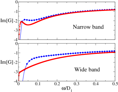
Figure 10: Imaginary part of the Green’s function for $D_{2}/D_{1}=0.18$, $U/D_{1}=2.00$, and $J=0$ as obtained by DMFT and with the PSCT.

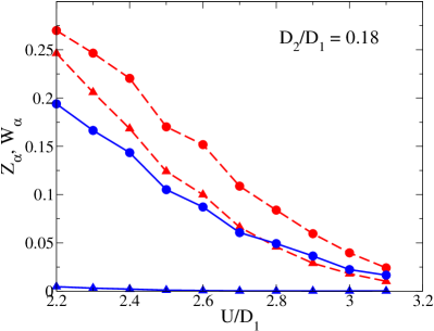
Figure 11: Quasiparticle residues $Z_{a}$ (triangles) and low-energy spectral weights $W_{a}$ (circles) as obtained by the PSCT with $J=0$. Dashed lines refer to the wide band, and continuous lines to the narrow one.

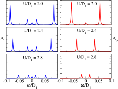
Figure 12: Low-energy part of the density of states of the wide band (left panels) and the narrow band (right panels) obtained within the PSCT for different $U/D_{1}$. The ratio of the bandwidth is $D_{2}/D_{1}=0.18$ and $J=0$.

In Fig. 11, we plot the PSCT values of the quasiparticle residues $Z_{1}$ and $Z_{2}$ as function of $U$ at $J=0$ for $D_{2}/D_{1}=0.18$, as well as of the full spectral weights, $W_{1}$ and $W_{2}$, inside the Mott Hubbard gap. In agreement with standard DMFT, we find a region where $Z_{2}$ is zero within our numerical accuracy, while $Z_{1}$ is still finite. Yet, the total spectral weights are both non zero. In Fig. 12, we draw the low-energy DOS for the two bands and various $U$’s.

VII Discussion and conclusions

In this work, we have studied by several techniques the properties of the Mott transition in an infinite-dimensional Hubbard model with two bands having the same center of gravity but different bandwidths, both in the presence and in the absence of the Hund’s exchange splitting $J$. We have shown that a variational calculation based on a Gutzwiller wave function predicts that the two bands may undergo different metal-insulator transitions both for $J=0$ and $J\not=0$: by increasing $U$, the narrower band ceases to conduct before the wider one. The necessary condition for this orbital-selective Mott transition is that the bandwidth ratio is lower than a critical value which increases with $J$, being 0.2 when $J=0$, see Fig. 3. This result would contradict both Liebsch, liebsch2003 ; liebsch2004 who claims that there is only a single Mott transition whatever is $J$ and the bandwidth ratio, as well as Koga and coworkers, koga2004 who instead suggest that the Mott transition is unique if $J=0$ but splits into two distinct ones as soon as $J\not=0$ for any value of the bandwidth ratio. The behavior of the quasiparticle residues as obtained by DMFT using exact diagonalization confirms, even quantitatively, the variational results, showing that the residue of the narrower band may vanish before the one of the wider band if the bandwidth ratio is sufficiently small, both for $J=0$ and $J\not=0$. Actually, an OSMT which occurs both in the absence and in the presence of an exchange splitting is somehow more conceivable, because the role of $J$ is model dependent. We notice that, in more general situations where the number of orbitals is greater than two and different from the number of electrons, as for instance in the case of $t_{2g}$ orbitals occupied by two or four electrons on average, the Coulomb exchange would instead compete against the angular momentum quenching which occurs in the OSMT scenario. Therefore, we suspect that the role of the Coulomb exchange might actually depend on the specific model.

However, a closer inspection to the low-energy spectral properties of the narrower band in the region where it is apparently insulating while the wider band still conducts poses doubts to the above simple scenario. The reason is that, in spite of a quasiparticle residue which is zero within our numerical accuracy, the narrower band has spectral weight inside the Mott-Hubbard gap, which scales like the quasiparticle residue of the wider band. In other words, the charge fluctuations which still occur in the wider band are transferred into the narrower one, as somehow predictable. This low-energy spectral weight is concentrated in two peaks symmetrically located around the chemical potential. Roughly speaking, the distance of each peak from the chemical potential is $2J$ plus a quantity of the order of the quasiparticle resonance width of the wider band. Due to our limited numerical resolution, we can not establish rigorously whether these two peaks (a) signal a narrow-gap semiconducting behavior, (b) signal a semimetallic behavior, with a power-law vanishing density of states, (c) or coexist with an extremely narrow resonance at the chemical potential, with a spectral weight well below our numerical accuracy, just like the single impurity does. Although the elements at our disposal do not definitely allow to discriminate among these three scenarios, yet one can recognize that some of them are more plausible than the others.

The first possibility (a) of a narrow-gap semiconductor seems very unlikely. Indeed, in this case, the gap between the two low-energy peaks would open large and then diminish as the quasiparticle resonance width of the wider band, by further increasing the repulsion $U$. Therefore, the insulating character of the narrower band would weaken by increasing $U$, which seems a bit odd.

Let us consider instead the scenario (b) of a semimetal. If taken literally, it would imply a vanishingly small local magnetic susceptibility, while we actually find a very large one, much larger than the local susceptibility of the wider band. However, a semimetallic behavior would imply, in our particle-hole symmetric case, a breakdown of Fermi liquid theory. nota Therefore, a power-law vanishing single-particle DOS might not necessarily conflict with almost free-spin excitations in a scenario in which Fermi liquid theory breaks down and for instance spin-charge separation emerges. Although it might represent a quite interesting circumstance, yet we could not find any physical arguments justifying such a non-Fermi liquid behavior. Therefore, we are tempted to discard it in favor of the more conservative scenario (c) in which the two peaks coexist with a narrow resonance which remains tied at the chemical potential, its spectral weight being smaller than our numerical accuracy. This resonance should disappear right at the same $U$ where the wider band ceases to conduct.

In any case, the rich structure of the low-energy spectrum, revealed by our study, highlights the subtlety of the present problem and could explain the discrepancies between previous studies. Further investigation is needed to confirm our speculation that the narrow resonance peak displayed by the single impurity survives the DMFT self-consistency.

- (1) A. Georges, G. Kotliar, W. Krauth, and M. J. Rozenberg, Rev. Mod. Phys. 68, 13 (1996).
- (2) J.E. Han, M. Jarrell, and D.L. Cox, Phys. Rev. B58, 4199 (1998); A. Koga, Y. Imai, and N. Kawakami, ibid. 66, 165107; Y. Ōno, M. Potthoff, and R. Bulla, ibid. 67, 35119 (2003); Th. Pruschke and R. Bulla, cond-mat/0411186.
- (3) N. Manini, G.E. Santoro, A. Dal Corso, and E. Tosatti, Phys. Rev. B66, 115107 (2002).
- (4) J.E. Han, Phys. Rev. B70, 054513 (2004); J.E. Han, O. Gunnarsson, and V.H. Crespi, Phys. Rev. Lett. 90, 167006 (2003); J.E. Han, E. Koch, and O. Gunnarsson, ibid. 84, 1276 (2000).
- (5) M. Capone, M. Fabrizio, C. Castellani, and E. Tosatti, Phys. Rev. Lett. 93, 047001 (2004); M. Capone, M. Fabrizio, C.Castellani, and E. Tosatti, Science 296, 2364 (2002).
- (6) A. Liebsch, Phys. Rev. Lett. 22, 226401 (2003)
- (7) A. Liebsch, Phys. Rev. B70, 165103 (2004)
- (8) A. Koga, N. Kawakami, T. M. Rice, and M. Sigrist, Phys. Rev. Lett. 92, 216402 (2004)
- (9) H.R. Krishnamurthy, J.W. Wilkins, and K.G. Wilson, Phys. Rev. B21, 1003 (1980); ibid. 1044 (1980).
- (10) J. Bünemann, W. Weber, and F. Gebhard, Phys. Rev. B57, 6896 (1998).
- (11) C. Attaccalite and M. Fabrizio, Phys. Rev. B68, 155117 (2003).
- (12) M. Caffarel and W. Krauth, Phys. Rev. Lett. 72, 1545 (1994).
- (13) G. Moeller, Q. Si, G. Kotliar, and M. Rozenberg, Phys. Rev. Lett. 74, 2082 (1995)
- (14) J.R. Schrieffer and P.A. Wolff, Phys. Rev. 149, 491 (1966).
- (15) In the presence of particle-hole symmetry, the chemical potential is strictly zero whatever is the interaction. On the other hand, if Fermi liquid theory holds, then . In this case, it turns out that the value of the DOS at the chemical potential should not be affected by and . Therefore, if one finds a different DOS from the bare one, that necessarily implies a breakdown of Fermi liquid theory.