Dynamics of a Quantum Phase Transition

Abstract

We present two approaches to the dynamics of a quench-induced phase transition in the quantum Ising model. One follows the standard treatement of thermodynamic second order phase transitions but applies it to the quantum phase transitions. The other approach is quantum, and uses Landau-Zener formula for transition probabilities in avoided level crossings. We show that predictions of the two approaches of how the density of defects scales with the quench rate are compatible, and discuss the ensuing insights into the dynamics of quantum phase transitions.

Studies of phase transitions traditionally focussed on equilibrium scalings of various properties near the critical point. The first major exception was an attempt to model the physics of the early Universe: Kibble Kib76 noted that cosmological phase transitions in a variety of field theoretic models lead to formation of topological defects (such as monopoles or cosmic strings) which may have observable consequences. One of us then pointed out Zur85a that analogues of cosmological phase transitions can be studied in the laboratory. In such experiments the equilibrium critical scalings predict various aspects of the non-equilibrium dynamics of symmetry breaking, including the density of residual topological defects Zur85a ; Zur96a .

These ideas led to the Kibble-Zurek mechanism (KZM), a theory of defect formation that uses the critical scalings of the relaxation time and of the healing length to deduce size ($\hat{\xi}$) of domains that choose the same “broken symmetry vacuum” Zur96a ; Kib03 . When the broken symmetry phase permits their existence, KZM predicts defects will appear with density of about one defect unit (e.g., one monopole or a $\hat{\xi}$-sized section of a string) per $\hat{\xi}$-sized domain. This KZM prediction has been tested, extended and refined with the help of numerical simulations LZ96a ; RH00a , and verified in a variety of increasingly sophisticated and reliable experiments in liquid crystals Chu92a ; Bow96a , superfluids He4a ; He4b ; He3 , superconductors Mon00a ; Car00 ; Man03 , and other systems Are00 .

A majority of the experimental data agree with KZM. One notable exception is the case of superfluid 4He, where initial reports of KZM vortices being detected He4a were retracted He4b after it turned out that stirring had inadvertently induced vorticity. In view of various uncertainties, it is still not clear whether 4He experiments are at odds with the numerics-assisted KZM predictions. Regardless, KZM provides a theory of the dynamics of second order phase transitions ranging from low temperature Bose-Einstein condensation to grand unification scales encountered in particle physics and cosmology.

In this paper we consider a barely explored problem: the dynamics of quantum phase transitions. Quantum many-body systems (e.g., Bose gases) can undergo thermodynamic phase transformation (such as Bose-Einstein condensation that follows evaporative cooling). KZM theory, developed to deal with thermodynamic phase transitions, applies in this case directly, even though the dynamics of Bose condensation is explicitly quantum AZ99a .

On the other hand, a quantum phase transition Sac99a (e.g., the Mott insulator-superfluid transition of bosons in a periodic lattice) is a change in the character of a system’s ground state which occurs as some parameter of its Hamiltonian passes critical value. For instance, lowering of the amplitude of the optical lattice induces Mott transition. Unlike thermodynamic transitions, quantum phase transitions involve only reversible unitary dynamics. Therefore, scaling arguments that work in thermodynamic transitions (where the order parameter is damped) may not be valid in the quantum case (but see DSBZ02 ; Dor03 ). Yet, dynamics of quantum phase transitions is interesting in its own right and has applications in quantum information processing Dor03 ; Cal04 .

We will study a quench-induced transition in the quantum Ising model. This model is regarded by Sachdev Sac99a as one of two canonical quantum phase transitions. It describes a chain of spins with the Hamiltonian:

$$H=-J(t)\sum_{l=1}^{N}\sigma_{l}^{x}-W\sum_{l=1}^{N-1}\sigma_{l}^{z}\sigma_{l+1}^{z}\ .$$ (1)

Here $\sigma_{l}^{x},~{}\sigma_{l}^{z}$ are Pauli operators, $W$ is the Ising coupling, and $J(t)$ is proportional to the strength of an external field that attempts to align spins with the $x$-axis.

The phase transition from the high-field state (all spins aligned with $x$, i.e., $|\rightarrow,\rightarrow,\dots,\rightarrow\rangle$) to the low-field ground state manifold – spanned by $|\uparrow,\uparrow,\dots,\uparrow\rangle$ and $|\downarrow,\downarrow,\dots\downarrow\rangle$, and doubly degenerate in the large $N$ limit – takes place when $J(t)=W$. Thus, relative coupling:

$$\epsilon(t)={J(t)/W}-1$$ (2)

is expected to play a role of the relative temperature $({T(t)\over T_{C}}-1)$ in system’s behavior near the critical point $T_{C}$.

Indeed, all relevant properties depend on the size of the gap ($\Delta$) between the ground state and the first excited state. As $N\rightarrow\infty$, the gap is:

$$\Delta=2|J(t)-W|=2W|\epsilon(t)|\ .$$ (3)

and sets an energy scale reflected in the relaxation time

$$\tau={\hbar/\Delta}={\hbar/{2W|\epsilon(t)|}}={\tau_{0}/|\epsilon(t)|}\ .$$ (4)

Divergence of $\tau$ near the critical point is the critical slowing down familiar from thermodynamic phase transitions.

The healing length is given by the product of the speed of sound $(c)$ and the relaxation time:

$$\xi=2Wa/\Delta(t)=a/|\epsilon(t)|=\xi_{0}/|\epsilon(t)|\ ,$$ (5)

where $c=2Wa/\hbar$ (see Sac99a ), and $a$ is the distance between spins. The divergence of $\xi$ near the critical point is analogous to critical opalescence.

The scaling of $\tau$ and $\xi$ suggests estimating the size of broken symmetry domains (i.e., regions of aligned spins) using the same approach that worked in thermodynamic transitions Zur85a ; Zur96a : Near the critical point “reflexes” of the system (measured by the relaxation time $\tau$) deteriorate, until – at the critical point, where $\tau=\infty$ – system cannot react at all. Yet, early in the quench $\tau$ is still small, and its state is still able to adjust to variations of the external parameter (e.g., $J$ or $T$). This suggests splitting the quench into the near-critical impulse regime and the quasi-adiabatic regime far from the critical point. Such split is the essence of KZM.

The instant ($\hat{t}$) when behavior of the system changes from adiabatic to impulse is of key importance. This happens when its reaction time (given by Eq. (4)) is the same as the timescale on which its Hamiltonian is changed. To calculate $\hat{t}$, we assume that the external bias field changes linearly with time, so that $\epsilon(t)=t/\tau_{Q}$. As the relative coupling changes on a timescale $\epsilon(t)/\dot{\epsilon}(t)=t$, the switch between adiabatic and impulse regimes occurs at the instants $\pm\hat{t}$ when relaxation time is equal to $t$,

$$\tau(\hat{t})=\ {\tau_{0}/|\epsilon(\hat{t})|}\ =\ \tau_{0}\tau_{Q}/\hat{t}\ =\ {{\epsilon(\hat{t})}/{\dot{\epsilon}(\hat{t})}}=\hat{t}$$ (6)

which yields

$$\hat{t}=\sqrt{\tau_{Q}\tau_{0}}=\sqrt{{\tau_{Q}\hbar}/{2W}}\ .$$ (7)

Typically, these two instants ($\pm\hat{t}$) separate evolution into three regimes. Initially, for $t<-\hat{t}$, the system’s state will adjust to the decreasing $J(t)$. However, at $t=-\hat{t}$ (before the critical point) this tracking of the instantaneous ground state of $H$ will cease. Evolution will re-start only at $+\hat{t}$ (after the critical point), with an initial state similar to the one “frozen out” at $-\hat{t}$.

In thermodynamic phase transitions fluctuations of the order parameter at $\hat{t}$ give rise to domains of size $\hat{\xi}$ given by the healing length at $-\hat{t}$. Using the relative coupling $\hat{\epsilon}$ at $\hat{t}$ we similarly calculate for the quantum Ising model:

$$\hat{\epsilon}\equiv\epsilon(\hat{t})={{\hat{t}}/\tau_{Q}}=\sqrt{\tau_{0}/\tau_{Q}};$$ (8)

$$\hat{\xi}\equiv\xi_{0}/{\hat{\epsilon}}=\xi_{0}\sqrt{\tau_{Q}/\tau_{0}}=a\sqrt{{2W\tau_{Q}}/{\hbar}}\ .$$ (9)

Note that this scaling differs from the $\hat{\xi}=\xi_{0}/\sqrt{\hat{\epsilon}}=\xi_{0}(\tau_{Q}/\tau_{0})^{1\over 4}$ predicted by non-relativistic mean-field theories for second order phase transitions Zur85a ; Zur96a .

Following KZM, we now expect appearance of $O(1)$ defects per $\hat{\xi}$. Their density should be therefore:

$$\hat{\nu}_{KZM}\simeq a/\hat{\xi}=\sqrt{{\hbar}/{2W\tau_{Q}}}.$$ (10)

This is only an estimate. Simulations of classical second order transitions yield defect densities that scale with $\tau_{Q}$ as predicted by KZM, but that can be lower by about an order of magnitude than $a/\hat{\xi}$: Defects can be separated not by $\hat{\xi}$ but by approximately 10 $\hat{\xi}$ (see LZ96a ).

Figure 1: Density of kinks ($\nu$) in quantum Ising model after a quench that starts in a ground state at $J=5W$ and ends at $J=0$, plotted versus the dimensionless quench rate $\tau_{0}/\tau_{Q}=\hbar v/4W^{2}$ for $N=50,60,70,80,90,100$ (solid lines; bottom to top). The simulation data are consistent with the scaling $\hat{\nu}_{KZM}\sim\sqrt{\tau_{0}/\tau_{Q}}$, Eq. (10), predicted by the Kibble-Zurek mechanism. (See Dor03 for details on the numerical method). Agreement improves with $N$; for 100 spins, a fit gives $\nu\sim\tau_{Q}^{-0.58}$ (dashed line). As in the classical case LZ96a Eq. (10) is an overestimate; the best fit is $\nu\simeq 0.16~{}\hat{\nu}_{KZM}$.

Figure 2: (a) Energies of lowest excitations (see Dor03 ) for $N=20$. The energies of the ground state and the first accessible excited state are the lowest (horizontal) solid line and the second lowest solid line. (b) (i) Quench time $\tau_{Q}/\tau_{0}=4W^{2}/\hbar v$ that yields $f$ of 99%, and (ii) the fidelity for a fixed $\tau_{Q}=200\hbar/W=400\tau_{0}$ as a function of the number of spins $N$ in the quantum Ising chain. A power-law fit to the data corresponding to $\tau_{Q_{99\%}}$ gives a power of 1.93 (LZF yields 2, as would KZM). The best fit for the fidelity with Landau-Zener dependence $f=1-\exp{\{{{-aW\tau_{Q}}/{\hbar N^{2}}}\}}$ yields $a\simeq 59$, compared to theoretical $a=2\pi^{3}\simeq 62$ based on the steeper slope in the marked energy level above ($a=4\pi^{3}\simeq 124$ when the more shallow slope in Fig. 2(a) consistent with Eq. (3) is taken). (c) Upper (dashed lines) and lower (solid lines) bounds on fidelity as a function of $\tau_{0}/\tau_{Q}=\hbar v/4W^{2}$ for $N=90$ (i), $N=70$ (ii), $N=50$ (iii), $N=30$ (iv). Fits to LZF (dotted lines) lie between these bounds, and for $f>0.6$ give $a\simeq 59$ (i), $59$ (ii), $57$ (iii), $54$ (iv).

This KZM paradigm should not be uncritically applied to quantum phase transitions. Above all, thermodynamic fluctuations are ‘real’. If they survive from before -$\hat{t}$, they can tip the balance at $+\hat{t}$, breaking symmetry right after the transition. It is hard to make an analogous argument for a quantum case equally convincing. Quantum fluctuations, exist, but they are virtual, so it is not obvious that they will have a similar symmetry breaking effect on the post-transition state. On a more prosaic note [as we shall see in Fig. 2(a)] the relevant gap (i.e., gap between the ground state and the first accessible excited state) is not the symmetric $\Delta$, Eq. (3). Rather, its slope is twice as large on the approaching side.

Nevertheless, Fig. 1 shows that number of kinks per spin – the residual kink density created by quenching the quantum Ising model scales approximately as $\sim 1/\sqrt{\tau_{Q}}$, just as predicted by Eq. (10). This holds throughout the region of KZM’s validity, i.e. where $\hat{\epsilon}$ is much less than 1 (so that the quench is quasi - adiabatic early on and at the end, but ‘impulse - like’ near the critical point, and thus at least one defect is expected). The prefactor $\sim 0.16$ [0.12 if the steeper slope on the approach in Fig. 2(a) is taken] is also not far from previous experience LZ96a .

Kibble-Zurek mechanism works in a quantum transition! Yet, in view of doubts about quantum fluctuations, an explicitly quantum treatment would be reassuring.

As $N\rightarrow\infty$, the gap ($\Delta$) – a salient feature of the quantum Ising model – disappears at the critical point in accord with Eq. (3). When $N<\infty$, this critical gap is small, but finite [see Fig. 2(a)]. This is of key importance for the remainder of our paper. Instead of calculating the density of defects in an infinite system, we shall compute size ($\tilde{N}$) of the largest spin chain likely to remain defect free (i.e., in a ground state) after a quench, as a function of quench timescale $\tau_{Q}$. For defect probability of $\sim$50%, inverse of $\tilde{N}$ is an estimate of defect density.

Excited eigenstates of $H$, Eq. (1), on the broken symmetry ($W>J$) side of the transition describe states of the spin chain in which the direction of symmetry breaking varies along the chain once, twice, etc. Sac99a . Thus, they represent states containing one, two, etc. “kinks”. The behavior of the energies of lowest excitations of $H$ in the vicinity of the critical point, [Fig. 2(a)], suggests avoided level crossing. Hence, it appears that phase transition dynamics in the quantum Ising model can be treated using the Landau-Zener formula LZ , or LZF. LZF gives the probability of exciting a system driven through an avoided level crossing:

$$p_{CHANGE}\simeq\exp\bigl{(}-{{\pi\hat{\Delta}^{2}}\over{2\hbar|v|}}\bigr{)}\ .$$ (11)

Here, $\hat{\Delta}$ is the minimum energy gap between the two levels, and $v$ is the quench velocity. That is, far away from the “point of the nearest approach”, $v=\dot{\Delta}$.

Using LZF we can compute the average size $\tilde{N}$ of a spin chain that is likely to remain in the ground state throughout the quench. In the adiabatic limit ($v\approx 0$), Eq. (11) predicts that the system will stay in the same energy eigenstate (i.e., the probability of switching levels will be vanishingly small). To quantify this Ref. Dor03 uses the fidelity, $f=|\langle\psi_{ACTUAL}|\psi_{GROUND}\rangle|^{2}$, which gives the probability that no defects will be produced. From LZF it follows that $p_{CHANGE}\simeq\exp\bigl{(}-{{\pi\hat{\Delta}^{2}}\over{2\hbar|v|}}\bigr{)}\simeq 1-f\$. Thus, the rate of a nearly defect - free quench (resulting in defects with probability 1-$f\ll 1$) is bounded:

$$|v|\leq{{\pi\hat{\Delta}^{2}}\over{2\hbar|\ln(1-f)|}}\ .$$ (12)

Below we will express $v$ using quench time $\tau_{Q}$ and $W$; $v=|\dot{\Delta}|=2\dot{J}(t)={2W/\tau_{Q}}$.

The lowest excited states are inaccessible – they have a different parity than the ground state, and $H$ conserves parity. The first accessible level has one kink for $J=0$. It gets to within $\hat{\Delta}=4\pi W/N$ for $N\gg 1$ above the ground state. With these ingredients using Eq. (12) we obtain:

$$|v|=|\dot{\Delta}|={{2W}\over\tau_{Q}}\leq{{\pi(4\pi W/\tilde{N})^{2}}\over{2\hbar|\ln(1-f)|}}\ .$$ (13)

It relates the size $\tilde{N}$ of a defect-free chain to quench time:

$$\tilde{N}\leq{2\pi}\sqrt{{\pi W\tau_{Q}}\over{\hbar|\ln(1-f)|}}={2\pi W}\sqrt{{2\pi}\over{\hbar v|\ln(1-f)|}}\ .$$ (14)

Figs. 2(b) and 2(c) show that LZF provides a good fit for $f>0.5$. This in not completely unexpected: Damski Dam04 recently proposed a ‘KZM approximation to LZF’ in an insightful paper. However, even upon closer inspection (work in progress DDZ ), such agreement between LZF in the setting which is not a standard avoided level crossing and the numerics might be still somewhat surprising.

When we compare the KZM and LZF predictions for defect density, we find:

$$\tilde{\nu}_{LZF}\simeq{1\over{\tilde{N}}}={1\over{2\pi}}\sqrt{{2|\ln(1-f)|}\over{\pi}}\times\hat{\nu}_{KZM}\ .$$ (15)

The two estimates of defect density exhibit the same scaling with the quench rate and with the parameters of $H$, Eq. (1). However, LZF predicts fewer defects than the “raw KZM estimate” ($\tilde{\nu}_{LZF}\simeq 0.14\times\hat{\nu}_{KZM}$ when $f$ is set – somewhat arbitrarily – to 0.5). This is no surprise; numerical simulations, experiments and analytic solutions to specific models, have shown that Eqs. (9) and (10) provide correct scalings, but tend to overestimate densities (see e.g. LZ96a ; Man03 ). Fig. 1 confirms that this is also true also for the quantum Ising model.

We note that while $\hat{\nu}_{KZM}$ and $\tilde{\nu}_{LZF}$ are closely related, they answer somewhat different questions. In particular, $\hat{\nu}_{KZM}$ does not depend on $f$. However, when less than one defect is expected in a chain, the number of defects is $\simeq 1-f$ and can be computed using LZF. Fig. 3 shows that LZF and KZM complement each other in this case, and jointly cover a wide range of quench rates.

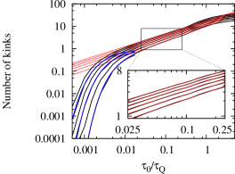
Figure 3: Number of kinks in chains ($N$=50,60,70,80,90,100, spins, bottom to top) after a quench versus the quench rate $\tau_{0}/\tau_{Q}=\hbar v/4W^{2}$. Both the scaling $\hat{\nu}\sim 1/\sqrt{\tau}_{Q}$ predicted by KZM (red lines), Eq. (10), and the LZF estimate $1-f$ (blue lines) are valid where expected. The red lines are linear fits in the range (0.025,0.25) yielding slopes between 0.66 and 0.58. The blue lines are the fit results from Fig. 2(c). Numerical data (obtained using the method developed in Dor03 ) include these used in Fig. 1. However, we now go beyond the expected range of validity of KZM: For quenches slow enough to create ‘less than a kink’ LZF provides reliable predictions, while very fast quenches are “all impulse”, and – according to KZM – the number of kinks should saturate, as is indeed seen.

We found that a quantum analogue of KZM, based on critical scalings, predicts the results of numerical simulations. As expected, KZM scaling holds when $\hat{\epsilon}<1$ – i.e., when the quench starts and ends in the adiabatic regime, but becomes impulse - like near the critical point. When the quench is so slow that it never acquires impulse - like character, LZF is accurate. We conclude that the two approaches work well in complementary regimes of quench rates, and predict the same scaling for the size of broken symmetry domains with quench time.

Exchanges of ideas with Robin Blume-Kohout and Bogdan Damski on both the substance and the presentation are acknowledged and appreciated, as is partial support by a Marie Curie Intra-European Fellowship within the 6th European Community Framework Programme, by a grant from NSA, and by the Austrian Science Foundation and EU Projects.

References

- (1) T. W. B. Kibble J. Phys., A9, 1387 (1976); Phys. Rep. 67, 183 (1980).
- (2) W. H. Zurek Nature 317, 505 (1985); Acta Physica Polonica B24, 1301 (1993).
- (3) W. H. Zurek Phys. Rep. 276, 177 (1996).
- (4) T. W. B. Kibble, pp. 3-36 in Patterns of Symmetry Breaking, H. Arodz et al., eds. (Kluwer Academic, New York, 2003).
- (5) P. Laguna & W. H. Zurek, Phys. Rev. Lett. 78, 2519 (1997); Phys. Rev. D58, 5021 (1998); A. Yates & W. H. Zurek, Phys. Rev. Lett 80, 5477 (1998); G. J. Stephens et al., Phys. Rev. D59, 045009 (1999).
- (6) N. D. Antunes et al., Phys. Rev. Lett., 82, 2824 (1999); M. B. Hindmarsh and A. Rajantie, Phys. Rev. Lett. 85, 4660 (2000).
- (7) I. L. Chuang et al., Science 251, 1336 (1991).
- (8) M. I. Bowick et al., Science 263, 943 (1994).
- (9) P. C. Hendry et al., Nature 368, 315 (1994).
- (10) M. E. Dodd et al., Phys. Rev. Lett. 81, 3703 (1998).
- (11) V. M. H. Ruutu et al. Nature 382, 334 (1996); C. Baürle et al., Nature 382, 332, (1996).
- (12) R. Monaco, J. Mygind, and R. J. Rivers, Phys. Rev. Lett. 89, 080603 (2002); Phys. Rev. B67, 104506 (2003).
- (13) R. Carmi, E. Polturak, and G. Koren, Phys. Rev. Lett. 84, 4966 (2000).
- (14) A. Maniv, E. Polturak, and G. Koren, Phys. Rev. Lett. 91, 197001 (2003).
- (15) S. Ducci et al., Phys. Rev. Lett. 83, 5210(1999); S. Casado et al., Phys. Rev. E63, 057301 (2001).
- (16) J. R. Anglin & W. H. Zurek Phys. Rev. Lett. 83, 1707 (1999).
- (17) S. Sachdev Quantum Phase Transitions (Cambridge University Press, Cambridge, England, 1999).
- (18) J. Dziarmaga et al., Phys. Rev. Lett. 88, 167001 (2002); and in Patterns of Symmetry Breaking, H. Arodz et al., eds. (Kluwer Academic, 2003)..
- (19) U. Dorner et al., Phys. Rev. Lett. 91, 073601 (2003).
- (20) T. Calarco et al., Phys. Rev. A 70, 012306 (2004).
- (21) L. D. Landau & E. M. Lifshitz, Quantum Mechanics (Pergamon, 1958); C. Zener, Proc. Roy. Soc. Lond. A137, 696 (1932).
- (22) B. Damski, Phys. Rev. Lett. 95, 035701 (2005).
- (23) B. Damski et al., (to be published).