Ground-State Decay Rate for the Zener Breakdown in Band and Mott Insulators

Abstract

Non-linear transport of electrons in strong electric fields, as typified by dielectric breakdown, is re-formulated in terms of the ground-state decay rate originally studied by Schwinger in non-linear QED. We discuss the effect of electron interaction on Zener tunneling by comparing the dielectric breakdown of the band insulator and the Mott insulator, where the latter is studied by the time-dependent density-matrix renormalization group. The relation with the Berry’s phase theory of polarization is also established.

Introduction — While there is a mounting body of interests in non-linear responses in many-body systems, the dielectric breakdown of Mott insulators is conceptually interesting in a number of ways. For band insulators the dielectric breakdown has been well understood in terms of the Zener tunnelingZener1934 across the valence and conduction bands, which triggers the breakdown. By contrast, non-linear properties in strongly correlated electron systems should be qualitatively different, since the excitation gap in the insulating side of Mott’s metal-insulator transition, arising from the electron-electron repulsion, is something totally different from the band gap in its origin and nature. Experimentally, Taguchi et al. observed a dielectric breakdown by applying strong electric fields to typical Mott insulators (quasi-one-dimensional cuprates, Sr₂CuO₃, SrCuO₂)tag . The present authors with Arita proposed theoretically that the phenomenon may be explained in terms of a Zener tunneling for many-body levels, and obtained the threshold field strength Oka2003 .

Now, there is an important difference between the Zener breakdowns in the band and Mott insulators: excitations (i.e., electrons and holes produced by the field) move freely in the former, while they must interact with surrounding electrons in the latter and become dissipated. In other words, while we have only to worry about the valence-conduction gap, we have to deal with many charge gaps among the many-body levels when the interaction is present. Several authors, including the present authors, have shown, with effective models, that a suppression of quantum tunneling due to the quantum interference should occur in many-level systems driven by external forces (see Gefan1987 ; Cohen2000 ; Oka2004a and refs. therein).

The tunneling rate, first obtained by Zener, gives the amount of the excitations, and is proportional to the leakage current if all the excitations are absorbed by electrodesZener1934 . So the rate is a crucial quantity, but theoretical studies have been quite scant: Even for band insulators, the quantity is only calculated for systems having a simple band dispersion. More importantly, Zener’s tunneling rate was based on a one-body WKB approach, so we must extend the formalism to many-body systems. Specifically, the actual breakdown should be related to the scattering between excited states in many-body systems as noted above. While this is shown to lead to a suppression of the current in a toy (quantum-walk) modelOka2004a , we are still badly in need of studies for microscopic models, since the existing calculation for the Hubbard modelOka2003 was limited to small systems (hence to short-time behaviors), while the long-time behavior, affected strongly by scattering between excited states, is in fact relevant.

In this Letter, we propose to determine the tunneling rate from the ground-state-to-ground-state transition amplitude, whose long-time asymptotic defines the effective Lagrangian. The effective-Lagrangian approach was evoked by Heisenberg and Euler in their study of quantum electrodynamics (QED) in strong electric fieldsHeisenberg1936 . This was extended by Schwinger to obtain the decay rate of the QED vacuumSchwinger1951 . It is well known that Schwinger’s electron-positron creation rate can be understood by the Landau-Zener mechanism (see e.g. Rau1996 ). What we have done here is the following: (i) We first express the effective Lagrangian for band insulators, which contains higher-order terms in the Landau-Zener’s tunneling probability. Since breakdown of band insulators is a well understood subject, the main aim of this section is to introduce the notations for later discussions. (ii) We then move on to a Mott insulator in strong electric fields. The ground-state decay rate is obtained for a microscopic (one-dimensional half-filled Hubbard) model with the time-dependent density-matrix renormalization groupVidal2004 ; White2004 . From this we determine the threshold electric field to construct the “dielectric breakdown phase diagram”. (iii) Finally we comment on an intriguing link between Heisenberg-Euler-Schwinger’s effective Lagrangian approach and a recent, Berry’s phase approach to polarization proposed in Refs.Resta1992 ; KingSmith1993 ; Resta1998 ; Resta1999 ; Nakamura2002 .

Dielectric Breakdown of a Band Insulator — We start with the dielectric breakdown of band insulators in an electric field $F$ within the effective-mass approximation. For simplicity we take a pair of hyperbolic bands $\varepsilon_{\pm}(\mbox{\boldmath$k$})=\pm\sqrt{V^{2}+v^{2}k^{2}}$ (considered here in $d$ spatial dimensions), where $V$ is the band gap, $-(+)$ represents the valence (conduction) band, and $v$ the asymptotic slope of the dispersion.

We first obtain the ground-state-to-ground-state transition amplitude with the time-dependent gauge in the periodic boundary condition. There, a time-dependent AB-flux measured by the flux quantum, $\phi(\tau)=FL\tau/h$ (with the electronic charge put equal to $e=1$, $L$ the system size) is introduced to induce an electric field $F$, which makes the Hamiltonian time dependent as $H(\phi(\tau))=\sum_{\bf{k},\alpha=\pm}\varepsilon_{\alpha}(\mbox{\boldmath$k$}+\frac{2\pi}{L}\phi(\tau)\mbox{\boldmath$e$}_{\parallel})c_{\alpha}^{\dagger}(\mbox{\boldmath$k$})c_{\alpha}(\mbox{\boldmath$k$}).$ Here $\mbox{\boldmath$e$}_{\parallel}$ is the unit vector parallel to $F$, and $c_{\alpha}^{\dagger}(\mbox{\boldmath$k$})$ the creation operator with spin indices dropped. If we denote the ground state of $H(\phi)$ as $|0;\phi\rangle$ and its energy as $E_{0}(\phi)$, the ground-state-to-ground-state transition amplitude is defined as

$$\Xi(\tau)=\langle 0;\phi(\tau)|\hat{T}e^{-\frac{i}{\hbar}\int_{0}^{\tau}H(\phi(s))ds}|0;\phi(0)\rangle e^{\frac{i}{\hbar}\int_{0}^{\tau}E_{0}(\phi(s))ds},$$ (1)

where $\hat{T}$ stands for the time ordering. The effective Lagrangian $\mathcal{L}(F)$ for the quantum dynamics is defined from the asymptotic behavior, $\Xi(\tau)\sim e^{\frac{i}{\hbar}\tau L^{d}\mathcal{L}(F)}$. The imaginary part of the effective Lagrangian gives the decay rate $\Gamma(F)/L^{d}=2\mbox{Im}\;\mathcal{L}(F)/\hbar$ à la Callan-ColemanCallanColeman1977 (see also Niu1998 ). $\Gamma(F)/L^{d}$ gives the rate of the exponential decay for an unstable vacuum (ground state), which, in the case of Zener tunneling, corresponds to the creation rate of electrons and holes. Originally, the creation rate for Dirac particles was calculated by Schwinger with the proper regularization methodSchwinger1951 . Below, we present a simpler derivation which can be extended to general band insulators.

The dynamics of the one-body model can be solved analytically, since we can cut the model into slices, each of which reduces to Landau-Zener’s two band modelLandau ; Zener . Namely, if we decompose the $k$ vector as $(\mbox{\boldmath$k$}_{\perp},k_{\parallel})$, where $\mbox{\boldmath$k$}_{\perp}$ ($k_{\parallel}$) is the component perpendicular (parallel) to $F$, each slice for a given $\mbox{\boldmath$k$}_{\perp}$ is a copy of Landau-Zener’s model with a gap $\Delta_{\rm band}(\mbox{\boldmath$k$})\equiv 2\sqrt{V^{2}+v^{2}k_{\perp}^{2}}$. The Landau-Zener transition takes place around the level anti-crossing on which $k_{\parallel}+\frac{2\pi}{L}\phi(\tau)$ moves across the Brillouin zone(BZ) in a time interval $\delta\tau=h/F$. The process can be expressed as a transition,

$$c_{+}^{\dagger}(\mbox{\boldmath$k$})\to\sqrt{1-p(\mbox{\boldmath$k$})}e^{-i\chi(\mbox{\boldmath$k$})}c_{+}^{\dagger}(\mbox{\boldmath$k$})+\sqrt{p(\mbox{\boldmath$k$})}c_{-}^{\dagger}(\mbox{\boldmath$k$}),$$

$$c_{-}^{\dagger}(\mbox{\boldmath$k$})\to-\sqrt{p(\mbox{\boldmath$k$})}c_{+}^{\dagger}(\mbox{\boldmath$k$})+\sqrt{1-p(\mbox{\boldmath$k$})}e^{i\chi(\mbox{\boldmath$k$})}c_{-}^{\dagger}(\mbox{\boldmath$k$}).$$ (2)

Here the tunneling probability for each $k$ is given by the Landau-Zener(LZ) formulaLandau ; Zener ,

$$p(\mbox{\boldmath$k$})=\exp\left[-\pi\frac{(\Delta_{\rm band}(\mbox{\boldmath$k$})/2)^{2}}{vF}\right],$$ (3)

while the phase $\chi(\mbox{\boldmath$k$})=-\theta(\mbox{\boldmath$k$})+\gamma(\mbox{\boldmath$k$})$ consists of the trivial dynamical phase, $\hbar\theta(\mbox{\boldmath$k$})=\int_{0}^{\delta\tau}\varepsilon_{+}(\mbox{\boldmath$k$}+\frac{2\pi}{L}\phi(s)\mbox{\boldmath$e$}_{\parallel})ds,$ and the Stokes phaseZener ; Kayanuma1993 ,

$$\gamma(\mbox{\boldmath$k$})=\frac{1}{2}\mbox{Im}\;\int_{0}^{\infty}ds\frac{e^{-i(\Delta_{\rm band}(\mbox{\boldmath$k$})/2)^{2}s}}{s}\left[\cot(vFs)-\frac{1}{vFs}\right].$$

The Stokes phase, a non-adiabatic extension of Berry’s geometric phase Berry1984 , depends not only on the topology of the path but also on the field strength $F$ Kayanuma1997 . In terms of the fermion operators the ground state is obtained by filling the lower band $|0;\phi\rangle=\prod_{\mbox{\boldmath$k$}}c^{\dagger}_{-}(\mbox{\boldmath$k$}-\frac{2\pi}{L}\phi\mbox{\boldmath$e$}_{\parallel})|{\rm vac}\rangle$, where $|{\rm vac}\rangle$ is the fermion vacuum satisfying $c_{\pm}(\mbox{\boldmath$k$})|{\rm vac}\rangle=0$. If we assume that excited charges are absorbed by electrodes electrode we obtain from eqs.(1), (2)

$$\mbox{Re}\;\mathcal{L}(F) = -F\int_{\rm BZ}\frac{d\mbox{\boldmath$k$}}{(2\pi)^{d}}\frac{\gamma(\mbox{\boldmath$k$})}{2\pi},$$

$$\mbox{Im}\;\mathcal{L}(F) = -F\int_{\rm BZ}\frac{d\mbox{\boldmath$k$}}{(2\pi)^{d}}\frac{1}{4\pi}\ln\left[1-p(\mbox{\boldmath$k$})\right],$$ (4)

where the dynamical phase $\theta$ cancels the factor $e^{\frac{i}{\hbar}\int_{0}^{\tau}E_{0}(\phi(s))ds}$ in eq.(1). Performing the $k$ integral in eq.(4) leads to the ground-state decay rate per volume for a $d$-dimensional hyperbolic band,

$$\Gamma(F)/L^{d} = \frac{F}{(2\pi)^{d-1}h}\left(\frac{F}{v}\right)^{(d-1)/2}$$ (5)

$$\times\sum_{n=1}^{\infty}\frac{1}{n^{(d+1)/2}}e^{-\pi n\frac{V^{2}}{vF}}\left[\mbox{erf}\left(\sqrt{\frac{nv\pi^{3}}{F}}\right)\right]^{d-1}.$$

To include the spin degeneracy we multiply this by $(2s+1)$ for a spin $s$ case.

If we compare eqs. (4), (5) with Heisenberg-Euler-Schwinger’s results of the nonlinear responses of the QED vacuum in strong electric fieldsHeisenberg1936 ; Schwinger1951 , two significant differences can be noticed. One is the error function appearing in eq.(5), which is due to the lattice structure (with the $k$ integral restricted to the BZ). In the strong-field limit ($F\to\infty$), the $F^{(d-1)/2}$ factor in eq.(5) is cancelled, and the tunneling rate approaches a universal function, $\Gamma(F)/L^{d}\to-\frac{F}{h}\ln\left[1-\exp\left(-\pi F_{\rm th}^{\rm band}/F\right)\right]$, independent of $d$. Another, quantitative difference appears in the Zener’s threshold voltageMuller1977 ; $F_{\rm th}^{\rm band}=V^{2}/va$ ($a$: lattice constant) for the dielectric breakdown is many orders smaller than the threshold for the QED instability $F^{\rm QED}=\frac{m_{e}^{2}c^{3}}{\hbar}\sim 10^{16}\;\mbox{V/cm}$.

Dielectric Breakdown of a 1D Mott Insulator — Having clarified the one-body case, we now discuss the effect of the strong electron correlation on a non-linear transport, i.e., the dielectric breakdown in the one-dimensional Mott insulator. We employ the half-filled Hubbard model in static electric fields. In the time-independent gauge, the Hamiltonian is $H+F\hat{X}$ with $H=-t\sum_{i\sigma}\left(c^{\dagger}_{i+1\sigma}c_{i\sigma}+\mbox{H.c}\right)+U\sum_{j}n_{j\uparrow}n_{j\downarrow},$ and $\hat{X}=\sum_{j}jn_{j}$ the position operatorResta1998 . When $F=0$ the ground state is a Mott insulator having a many-body energy gap so far as $U>0$Lieb:1968AM ; Woynarovich1982all .

After a strong electric field is switched on at $\tau=0$, quantum tunneling begins to take place, first from the ground state to the lowest excited states, and then to higher ones. The tunneling to the lowest excited states, which dominates the short-time behavior, has been shown to be understood with the Landau-Zener formula (see eq.(8)) Oka2003 , but it is the long-time behavior that should be relevant to the actual breakdown.

The ground-state-to-ground-state transition amplitude is, in the time-independent gauge,

$$\Xi(\tau)=\langle 0|e^{-\frac{i}{\hbar}\tau\left(H+F\hat{X}\right)}|0\rangle e^{\frac{i}{\hbar}\tau E_{0}},$$ (6)

where we denote the ground state of $H$ as $|0\rangle$ and its energy as $E_{0}$. The transition amplitude is calculated here numerically by first obtaining $|0\rangle$ in the open boundary condition with the density-matrix renormalization group (DMRG) method, and then solving the time-dependent Schrödinger equation for the many-body system with the time-dependent DMRG Vidal2004 ; White2004 . The ground-state decay rate $\Gamma(F)/L$ in strong electric fields $F$ is then obtained from the asymptotic behavior of $\Xi(\tau)$.

Figure 1: (a) The temporal evolution of the ground-state survival probability $|\Xi(\tau)|^{2}$ after the electric field $F$ is switched on at $\tau=0$ in the 1D half-filled Hubbard model with $U/t=3.5$, obtained with the time-dependent DMRG for $L=50$ with the size of the DMRG Hilbert space $m=150$ and the time step $d\tau=0.02$. The dashed line represents $-\ln|\Xi(\tau)|^{2}=\Gamma(F)\tau+c$ for $F/t=0.17$. (b) The decay rate versus $F$ in the half-filled Hubbard model. Dashed line is a fit to eq.(7), where $F_{\rm th}^{\rm Mott}(U)$ is the threshold.

Figure 1(a) shows the temporal evolution of the ground-state survival probability $|\Xi(\tau)|^{2}$ for a system with $U/t=3.5$. We notice that, as time increases, the slope of $-\ln|\Xi(\tau)|^{2}$ decreases after an initial stage. The slope is proportional to the decay rate, so its decrease implies a suppression of the tunneling. We can regard this as evidence that charge excitations are initially produced due to the Zener tunneling, but that, as the population of the excitations grows, scattering among the excited states become important. This results in the “pair annihilation” of carriers, which acts to suppress the tunneling rate. We have determined $\Gamma(F)$ from the long-time behavior with a fitting $-\ln|\Xi(\tau)|^{2}=\Gamma(F)\tau+{\rm const}$.

The decay rate per length $\Gamma(F)/L$ is plotted in Fig.1(b), where we have varied the system size ($L=30,50$) to check the convergence. $\Gamma(F)/L$ is seen to remain vanishingly small until the field strength exceeds a threshold. To characterize the threshold $F_{\rm th}(U)$ for the breakdown we can evoke the form obtained above for the one-body system (eq.(5)),

$$\Gamma(F)/L=-\frac{2F}{h}a(U)\ln\left[1-\exp\left(-\pi\frac{F_{\rm th}^{\rm Mott}(U)}{F}\right)\right]$$ (7)

(with a factor of $2$ recovered for the spin degeneracy). The interest here is whether this holds when we replace $F_{\rm th}^{\rm band}$ with $F_{\rm th}^{\rm Mott}(U)$. The factor $a(U)$ is a parameter representing the suppression of the quantum tunneling. The dashed line in Fig.1 (b) is the fitting for $U/t=3.5$, where we can see that the fitting, including the essentially singular form in $F$, is surprisingly good, given a small number of fitting parameters. The value of $a(U)$ turns out to be smaller than unity (taking between $0.77$ to $0.55$ as $U/t$ is increased from $2.5$ to $5.0$).

In Fig.2 we plot the $U$ dependence of $F_{\rm th}^{\rm Mott}$. The dashed line is the prediction of the Landau-Zener formula (see eq.(3))

$$F_{\rm th}^{\rm LZ}(U)=\frac{[\Delta_{\rm charge}(U)/2]^{2}}{v},$$ (8)

which was first applied to the dielectric breakdown of the half-filled Hubbard model in ref.Oka2003 . For the size of the Mott (charge) gap we use the Bethe-ansatz result: $\Delta_{\rm charge}(U)=\frac{8t}{U}\int_{1}^{\infty}\frac{\sqrt{y^{2}-1}}{\sinh(2\pi yt/U)}dy$Lieb:1968AM ; Woynarovich1982all with $v/t=2$.

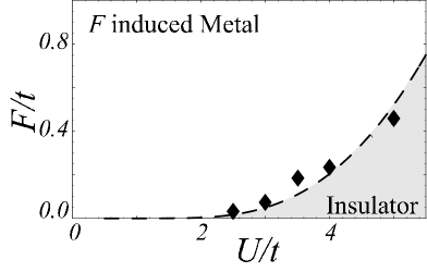
Figure 2: The dielectric breakdown phase diagram on $(U,F)$ for the one-dimensional Hubbard model. The symbols are the threshold $F^{\rm Mott}_{\rm th}(U)$ obtained by fitting the decay rate $\Gamma(F)/L$ to eq.(7)), while the dashed line is the prediction $F=F_{\rm th}^{\rm LZ}(U)$ of the Landau-Zener formula eq.(8).

So the overall agreement between the threshold for the Hubbard model and eq.(8) is again confirmed, but to be more precise we note the following. Since the scattering among charge excitations suppresses tunneling, the threshold for the breakdown in interacting systems is expected to be larger than the Landau-Zener prediction (eq.(8)). It was proposed in Oka2004a that the wave function in electric fields just below the threshold is localized (on energy axis) around the ground state, which physically corresponds to a state where the production and annihilation of excited states are balanced due to the quantum interference. The $F/t=0.11$ result in Fig.1(a) is typical of such states, where $-\ln|\Xi(\tau)|^{2}$ first increases but soon saturates. When we further increase the field strength, the production exceeds the annihilation, which leads to an exponential decay of the ground state with rate $\Gamma(F)/L$. The system is now metallic in the sense that there are carriers that contribute to transport.

As for the question of whether the dielectric breakdown in the non-linear regime may be regarded as a true transition, future studies should be needed. The form (eq.(7)) we used for fitting the tunneling rate assumes that the transition is a smooth crossover around $F\sim F_{\rm th}^{\rm Mott}(U)$. However, the toy (quantum-walk) model calculation indicates that the breakdown of many-body systems is a localization-delocalization transitionOka2004a . This suggests that the tunneling rate and other physical quantities may become singular at the breakdown field, in which case the $I$-$V$ characteristics exhibits a jump or a kink. In our numerical calculation, while we do find an indication of localization for $F/t=0.11$ in Fig.1(a), we observe no singularities in the tunneling rate. So, future calculations will reveal the nature of the transition around the breakdown.

Finally, we comment on the relation of the effective Lagrangian approach with earlier approaches, especially the Berry’s phase theory of polarizationResta1992 ; KingSmith1993 ; Resta1998 ; Resta1999 ; Nakamura2002 . There, the ground-state expectation value of the twist operator $e^{-i\frac{2\pi}{L}\hat{X}}$, which shifts the phase of electrons on site $j$ by $-\frac{2\pi}{L}j$ Nakamura2002 , plays a crucial role. It was revealed that the real part of a quantity

$$w=\frac{-i}{2\pi}\ln\langle 0|e^{-i\frac{2\pi}{L}\hat{X}}|0\rangle$$ (9)

gives the electric polarization, $P_{\rm el}=-\mbox{Re}w$ Resta1998 , while its imaginary part gives a criterion for metal-insulator transition, i.e., $D=4\pi\mbox{Im}w$ is finite in insulators and divergent in metals Resta1999 . The effective action in the present work is regarded as a non-adiabatic (finite electric field) extension of $w$. To give a more accurate argument, recall that the effective Lagrangian can be expressed as $\mathcal{L}(F)\sim\frac{-i\hbar}{\tau L}\ln\left(\langle 0|e^{-\frac{i}{\hbar}\tau(H+F\hat{X})}|0\rangle e^{\frac{i}{\hbar}\tau E_{0}}\right)$ for $d=1$. Let us set $\tau=h/LF$ and consider the small $F$ limit. For insulators we can replace $H$ with the ground-state energy $E_{0}$ to have

$$\mathcal{L}(F)\sim wF$$ (10)

in the linear response regime. Thus, the real part of Heisenberg-Euler’s expressionHeisenberg1936 for the non-linear polarization $P_{\rm HE}(F)=-\frac{\partial\mathcal{L}(F)}{\partial F}$ naturally reduces to the Berry’s phase formula $P_{\rm el}$ in the $F\to 0$ limit (cf. eq.(4)). Its imaginary part, which is related to the decay rate as $\mbox{Im}P_{\rm HE}(F)=-\frac{\hbar}{2}\frac{\partial\Gamma(F)/L}{\partial F}$, reduces to $-\frac{D}{4\pi}$ and gives the criterion for the transition, originally proposed for the zero field case.

We thank R. Arita for illuminating discussions. TO acknowledges M. Nakamura, S. Murakami, N. Nagaosa, and D. Cohen for helpful comments. Part of this work was supported by JSPS.

After the completion of this work, we came to notice a recent paper by Green and SondhiGreen2005 , where non-linear transport near a superfluid/Mott transition is studied from the point of view of the Schwinger mechanism.

^∗ Present address: CERC, National Institute of Advanced Industrial Science and Technology, Tsukuba Central 4, Tsukuba, Ibaraki, 305-8562 Japan.

References

- (1) C. Zener, Proc. Roy. Soc. A 145, 523 (1934).
- (2) Y. Taguchi, T. Matsumoto, and Y. Tokura, Phys. Rev. B 62, 7015 (2000).
- (3) T. Oka, R. Arita, and H. Aoki, Phys. Rev. Lett. 91, 66406 (2003).
- (4) Y. Gefen and D. J. Thouless, Phys. Rev. Lett. 59, 1752 (1987).
- (5) D. Cohen and T. Kottos, Phys. Rev. Lett. 85, 4839 (2000).
- (6) T. Oka, N. Konno, R. Arita, and H. Aoki, Phys. Rev. Lett. 94, 100602 (2005).
- (7) W. Heisenberg, and H. Euler, Z. Physik 98, 714 (1936).
- (8) J. Schwinger, Phys. Rev. 82, 664 (1951).
- (9) J. Rau, and B. Müller, Physics Report 272, 1 (1996).
- (10) G. Vidal, Phys. Rev. Lett. 93, 040502 (2004).
- (11) S. R. White and A. E. Feiguin, Phys. Rev. Lett. 93, 076401 (2004).
- (12) R. Resta, Ferroelectrics 136, 51 (1992).
- (13) R. D. King-Smith and D. Vanderbilt, Phys. Rev. B 47, R1651 (1993).
- (14) R. Resta, Phys. Rev. Lett. 80, 1800 (1998).
- (15) R. Resta and S. Sorella, Phys. Rev. Lett. 82, 370 (1999).
- (16) M. Nakamura and J. Voit Phys. Rev. B 65, 153110 (2002).
- (17) C. G. Callan, Jr. and S. Coleman, Phys. Rev. D 16, 1762 (1977). The ground-state energy in their paper corresponds to in our notation.
- (18) Q. Niu and M.G. Raizen, Phys. Rev. Lett. 80, 3491 (1998).
- (19) L.D. Landau, Phys. Z. Sowjetunion 2, 46 (1932).
- (20) C. Zener, Proc. R. Soc. Lond. Ser. A 137, 696 (1932).
- (21) Y. Kayanuma, Phys. Rev. B 47, 9940 (1993).
- (22) M.V. Berry, Proc. R. Soc. A 392, 45 (1984).
- (23) Y. Kayanuma, Phys. Rev. A 55, R2495 (1997).
- (24) This means that the state vector after is since the term disappears.
- (25) B. Müller W. Greiner, and J. Rafeski, Phys. Lett. A 63, 181 (1977).
- (26) E. H. Lieb and F. Y. Wu, Phys. Rev. Lett 21, 192 (1968).
- (27) F. Woynarovich, J. Phys. C 15, 85 (1982); 15, 97 (1982); 16, 5293 (1983).
- (28) A. G. Green and S. L. Sondhi, cond-mat/0501758.